
 Submit a Paper
 Propose a Special lssue
 Open Access
ARTICLE
Parameters Optimization and Performance Evaluation of the Tuned Inerter Damper for the Seismic Protection of Adjacent Building Structures
1 Key Laboratory of Intelligent Underground Detection Technology, School of Civil Engineering, Anhui Jianzhu University, Hefei, 230601, China
2 Chengnan College, Changsha University of Science and Technology, Changsha, 410015, China
* Corresponding Author: Xiaofang Kang. Email:
(This article belongs to the Special Issue: Vibration Control and Utilization)
Computer Modeling in Engineering & Sciences 2024, 138(1), 551-593. https://doi.org/10.32604/cmes.2023.029044
Received 28 January 2023; Accepted 22 May 2023; Issue published 22 September 2023
 View Full Text
 Download PDF
Abstract
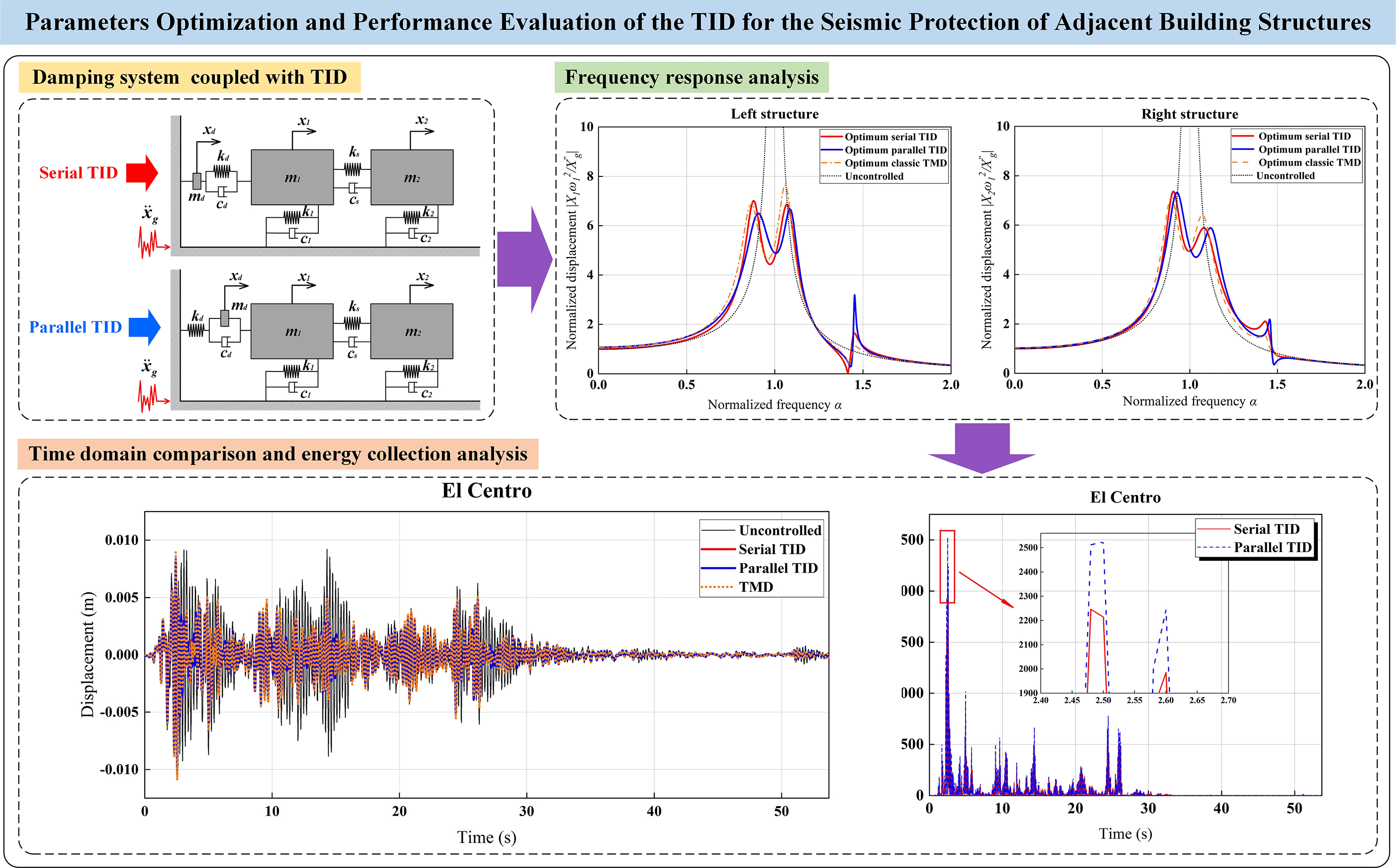
In order to improve the seismic performance of adjacent buildings, two types of tuned inerter damper (TID) damping systems for adjacent buildings are proposed, which are composed of springs, inerter devices and dampers in serial or in parallel. The dynamic equations of TID adjacent building damping systems were derived, and the H2 norm criterion was used to optimize and adjust them, so that the system had the optimum damping performance under white noise random excitation. Taking TID frequency ratio and damping ratio as optimization parameters, the optimum analytical solutions of the displacement frequency response of the undamped structure under white noise excitation were obtained. The results showed that compared with the classic TMD, TID could obtain a better damping effect in the adjacent buildings. Comparing the TIDs composed of serial or parallel, it was found that the parallel TIDs had more significant advantages in controlling the peak displacement frequency response, while the H2 norm of the displacement frequency response of the damping system under the coupling of serial TID was smaller. Taking the adjacent building composed of two ten-story frame structures as an example, the displacement and energy collection time history analysis of the adjacent building coupled with the optimum design parameter TIDs were carried out. It was found that TID had a better damping effect in the full-time range compared with the classic TMD. This paper also studied the potential power of TID in adjacent buildings, which can be converted into available power resources during earthquakes.Graphic Abstract
Keywords
Since Lee et al. first proposed the method of vibration control for civil structures in 1972 [1], the theory and method of vibration control have been developed rapidly. In order to deal with structural vibration problems caused by wind load or earthquake load, a series of control strategies have been formed, including active control, passive control, hybrid control, and intelligent control [2]. Among them, passive vibration control is widely used in engineering practice because of its high stability, low cost, good control effect, and easy realization [3,4]. The design of classic tuned mass damper (TMD) consists of a mass block, spring and viscous damper, which is a reliable structural vibration control device [5]. Kareem et al. took high-rise buildings subjected to wind load as an example, introduced the application of TMDs in Australia, Canada, China, Japan, and the United States in recent years, and showed that TMD had superior seismic performance [6]. However, for TMD, to obtain better and more robust control performance, it is necessary to use a larger auxiliary mass, that is, to increase the mass ratio of TMD to the controlled structure, which is often restricted by site conditions or costs [7]. In order to solve the problems encountered in the practical application of TMD, researchers have developed many new dampers based on the existing TMD research, including electromagnetic inertial mass damper (EIMD) [8,9], rotational inertial damper (RID) [10,11], rotational inertial double-tuned mass damper (RIDTMD) [12–14], tuned mass damper inerter (TMDI) [15–17], tuned liquid inerter system (TLIS) [18], tuned inerter damper (TID) [19–23], tuned mass-inerter damper (TMID) [24], tuned fluid inerter (TFI) [25,26], clutching inerter damper (CID) [27], etc. These dampers introduced a promising passive vibration control device, namely inerter device.
Inerter device is a mechanical device with two ends which was first proposed by Smith in 2002 [28]. Its characteristic is that the applied inerter force is proportional to the relative acceleration between the two ends, and it usually consists of rack and pinion, ball screw and hydraulic mechanism [12,29,30]. Inerter devices have significant mass amplification effect, and the effective mass produced can exceed 100 times of its physical mass [13,31,32]. The principle of the inerter device is that it can transform the linear motion of both ends of the device into the rotational motion of the flywheel when an earthquake occurs, resulting in considerable inerter [33–35]. For example, Ikago et al. realized an apparent mass of 300 kg with a ball screw device with a physical mass of only 2 kg [36], Javidialesaadi et al. designed and produced a ball screw mechanism with a physical mass of only 2 kg to produce an effective mass of 350 kg [13]. It can be seen that in order to produce an equivalent effective mass, the actual physical mass of the inerter device is far less than that of the traditional TMD. In addition, the research also showed that when the TID is placed at the bottom of the main structure, the performance of the TID is the best, which is opposite to the TMD that must be placed at the position where the maximum displacement occurs, that is, the top of the structure [22]. TID can obtain a large inerter mass ratio without increasing the physical mass, so it is considered that TID can replace the traditional TMD and be applied in engineering practice. Based on inerter device, Dai et al. explored the optimal design of Maxwell tuned-mass-damper-inerter (M-TMDI) to mitigate vortex-induced vibration (VIV) of bridges. Based on a two-DOF system, the optimal parameters of a specific M-TMDI, in which the end of the inerter is connected to the fixed ground, are analytically given using the inerter location as a design variable [37]. In addition, Dai et al. aimed at the impact of the location of inerter on the control performance of tuned mass-damping-inerter (TMDI) in wind-induced vibration mitigation of flexible structures, discussed the control effect, optimum design parameters, and high-mode damping effects of the TMDI [38]. Different types of control devices based on inerter devices are also used in base isolated structures. TIDs are installed at the bottom of the structure to further reduce the displacement of isolated floors and the inter story displacement of superstructure [35,39,40]. Among them, the inerter device based on the generator device can collect energy while reducing the displacement of the upper structure, realizing the trade-off between the two contradictory goals of energy collection and vibration control [35]. Gonzalez-Buelga et al. proposed a circuit containing both damping and energy collection effects, and connected it with the electromagnetic transducer to synthesize TID, which also achieved the dual goals of damping and energy collection [41]. Unlike TMD driven by the absolute motion of the damper, TID is driven by the relative motion between the two ends of the device, which actually provides conditions for the corresponding energy collection mode of TID [42].
In order to achieve the best control effect of the vibration control device, different types of optimization methods have been proposed, including the most commonly used method, namely H2 norm optimization. The H2 optimization criterion was first proposed by Crandall and Mark in 1963 and applied to the design of dynamic vibration absorbers (DVAs), with the goal of reducing the total vibration energy of the system at all frequencies [43]. It can be understood that if the vibration control system is subjected to random excitation, that is, the excitation contains an infinite number of frequencies, then it is unnecessary to consider only the resonance frequency of the system. Under this optimization criterion, the area under the frequency response curve of the system (called H2 norm) is the smallest [44]. In the study of vibration control of adjacent buildings based on inerter, Palacios-Quiñonero et al. proposed a computational strategy to design inerter-based multi-actuation systems for the seismic protection of adjacent structures based on an H∞ cost-function and used a constrained global-optimization solver to compute parameter configurations with high-performance characteristics. The research results fully demonstrate the flexibility and effectiveness of the proposed design methodology, and clearly show the superior performance and robustness of the TID actuation systems [45]. Djerouni et al. proposed a new configuration of TMDIs with the goal of studying the seismic response of two adjacent buildings and the pounding distance between them. The results show that the proposed method is effective and better than the existing TID configuration, filling a gap in the research of investigating the effectiveness of TMDI in controlling seismic pounding and the impact of ground motion variability [46]. Taking adjacent buildings as controlled structures, this paper investigated the vibration control performance of serial TID and parallel TID in adjacent buildings. Also, the analytical solutions of the optimum frequency ratio and damping ratio of structural vibration control under random excitation were obtained by using the H2 norm optimization method. In addition, for the convenience of analysis, the random excitation used in this paper is white noise excitation when analyzing the frequency response of the system.
The main contents of this paper are summarized as follows: First, the analytical solutions of the optimum frequency ratio and the optimum damping ratio of adjacent building structures under the coupling of serial TID and parallel TID were obtained by using the H2 optimization method. Secondly, the influence of different structural parameters on the optimum solutions was studied. Then, the classic TMD was introduced to compare with the two types of TID, and the frequency response of adjacent building structures under different damper coupling was analyzed. At the same time, the influence of damper mass was also considered. Then, by changing the optimum frequency ratio and the optimum damping ratio, the robust performance of vibration of adjacent buildings under TID coupling was analyzed. Finally, four types of seismic waves were used to analyze the time history of vibration control of adjacent building structures under two types of TIDs and classic TMD coupling, and the time history of energy collection of adjacent building structures under two types of TIDs coupling was analyzed.
2.1 Simplified Model of Adjacent Buildings
As shown in Fig. 1a is the simplified model of adjacent buildings, where

Figure 1: Simplified schematic graph of adjacent building structures
Adding ball screw mechanism (including shell and linear guide rail), flywheel and rotary generator inside the damper can transform the relative linear motion between the structure and the ground into rotation when an earthquake occurs, and drive the flywheel and generator to collect energy [35]. The rotating generator and flywheel drive the inerter mass to rotate, and generate resistance to the driving structure. The damper is elastically installed with the structure, which is equivalent to a spring. Fig. 2a shows a simplified model of the inerter device. It is characterized in that the generated force is proportional to the difference of acceleration at both ends [22]. The mechanical equation can be expressed as:
where

Figure 2: Inerter device and two types of inerter-based damper models: (a) Inerter device; (b) Serial TID; (c) Parallel TID
According to Section 2.2, considering different connection modes, two damper models with different configurations based on inerter are formed. According to the different positions of

Figure 3: The damping system of adjacent buildings coupled with TID: (a) Serial TID damping system; (b) Parallel TID damping system
3 Parameter Optimization Based on H2 Norm Criterion
According to the coupled damping system in Fig. 3, the dynamic balance equation of the system can be listed. We stipulate that the structure on the left which connected to TID is the left structure, and the structure on the right of adjacent buildings is the right structure, and they will be distinguished by left structure and right structure in subsequent expressions.
According to the balance principle of force, the dynamic balance equation can be obtained as follows:
After dimensionless transformation by Laplace transform, the following results are obtained:
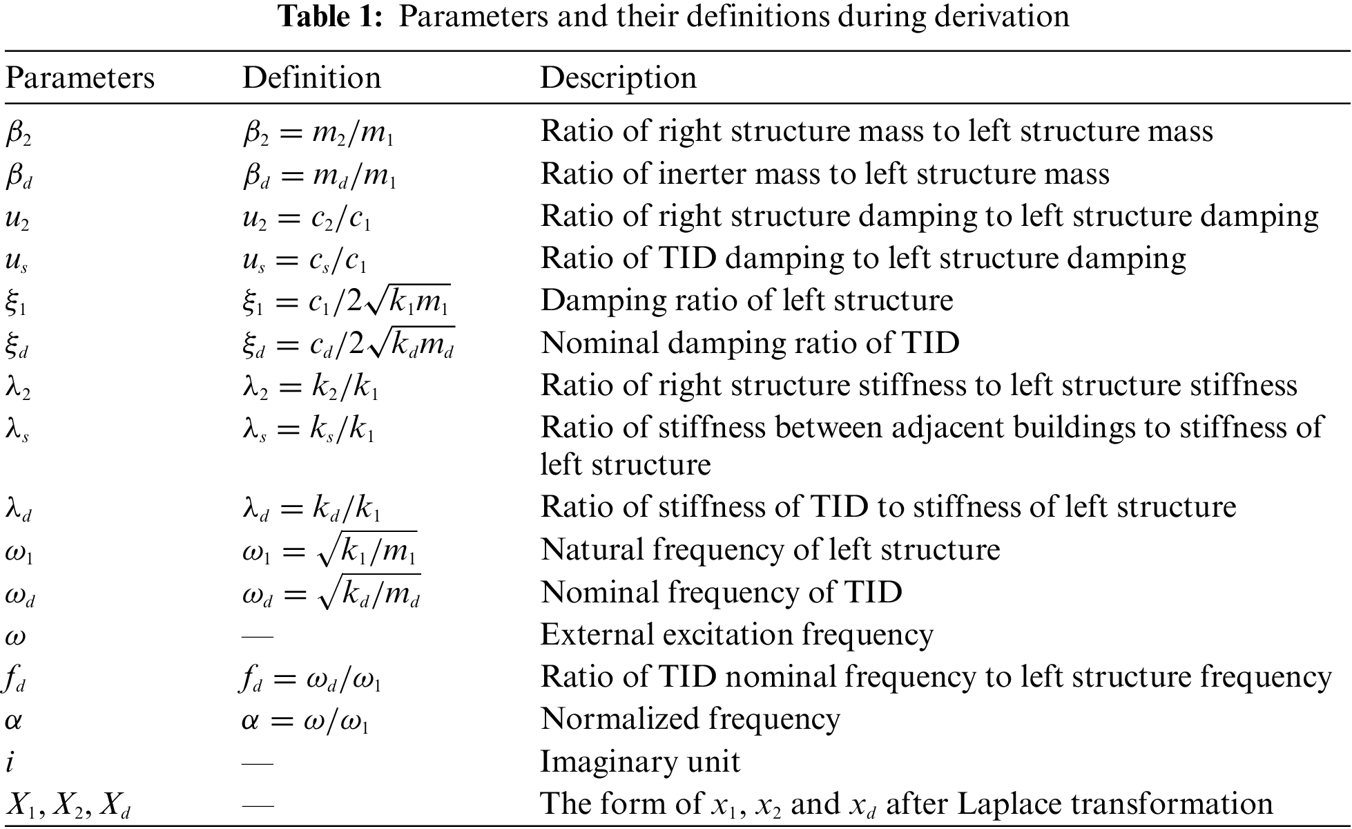
Define some new parameters for the next transformation. The defined parameters are shown in Table 1. After substituting them into Eq. (3), there are:
According to the balance principle of force, the dynamic balance equation can be obtained as follows:
Similar to the serial TID, it can be obtained from Table 1 and Eq. (5) as follows:
3.2 Solution of the Transfer Function
Before H2 optimization, it is necessary to obtain the normalized displacement transfer functions of the left structure and the right structure under different connection modes of TID. Solve Eqs. (4) and (6) to obtain the following results.
(1) Left structure
where the superscript “s” denotes serial connection, and the subscript “1” denotes the left structure, and its numerator and denominator coefficients are shown in Appendix A.
(2) Right structure
where the superscript “s” denotes serial connection, the subscript “2” denotes the right structure, the denominator coefficient is the same as the left structure, and the numerator coefficient is shown in Appendix B.
(1) Left structure
where the superscript “p” denotes parallel connection, the subscript “1” denotes the left structure, and its numerator and denominator coefficients are shown in Appendix C.
(2) Right structure
where the superscript “p” denotes parallel connection, the subscript “2” denotes the right structure, the denominator coefficient is the same as the left structure, and the numerator coefficient is shown in Appendix D.
In order to verify the damping effect of different types of TID coupled with adjacent buildings, H2 optimization method is used to optimize the parameters of vibration control system, and the external excitation used in this paper is white noise excitation. If the evaluation index is defined as
where
To simplify the analysis, take the damping between the left structure and the right structure as 0, that is, from Table 1:
(1) Serial TID
After substituting Eqs. (7) and (8) into the evaluation index
where the superscript “s” denotes serial connection, the subscripts “1, 2” denote the left structure and the right structure, respectively.
(2) Parallel TID
After substituting Eqs. (9) and (10) into the evaluation index
where the superscript “p” denotes parallel connection, the subscripts “1, 2” denote the left structure and the right structure, respectively.
In order to obtain the optimum solutions, the evaluation index
(1) Serial TID
By solving Eqs. (16) and (17), respectively, we can get the optimization results (Eq. (18) represents the left structure, and Eq. (19) represents the right structure):
Here, it is necessary to point out:
(2) Parallel TID
By solving Eq. (21) and by Eq. (20), we can get the optimization results of the left structure under the parallel TID coupling are:
When solving Eq. (22), this equation group is converted into the solution of Eq. (24), which includes:
where
see Appendix J for the specific form of
By solving Eq. (24), and with Eq. (20), the optimization results of the right structure under parallel TID coupling are obtained as follows:
where
Before parameters analysis, it is necessary to give specific values of parameters that have not been optimized. In order to facilitate the optimization analysis, the mass, damping and stiffness of the left structure and the right structure are determined to be consistent in this section, that is, Table 1 shows:
In Section 3.3.2, the process and results of parameter optimization are given. However, many of the optimization results have root signs. According to the mathematical knowledge, all values under the root sign should be greater than or equal to 0. After considering all the optimization results, it is found that the conditions affecting the value of
To determine the value of
Combining Eqs. (H1) and (H2), the image of Eq. (28) is drawn as shown in Fig. 4. It can be seen from the figure that if
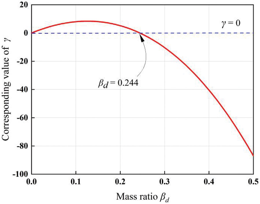
Figure 4: Analysis of the value of mass ratio
It was found during parameter optimization that if
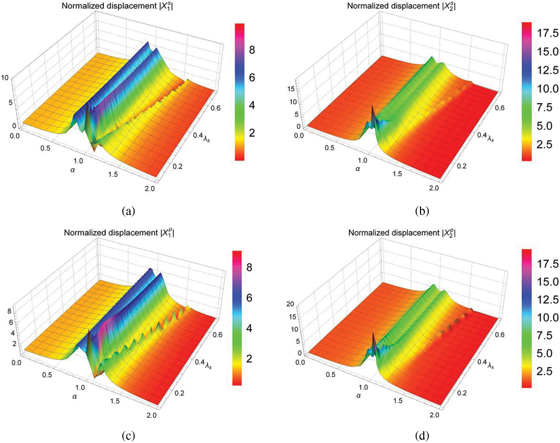
Figure 5: Three-dimensional graphs of normalized displacement when the stiffness ratio
As can be seen from Fig. 5, when
4.1.3 Verification of Optimization Results
After the values of two key parameters

Figure 6: Three-dimensional graphs of evaluation index
It can be seen from Figs. 6a and 6b that the evaluation indexes
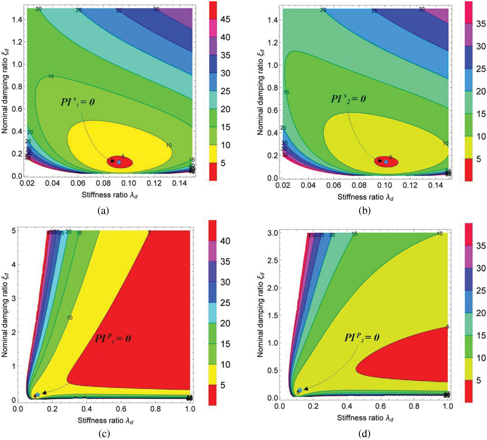
Figure 7: The contour graphs of evaluation index
From the closure of the contour graphs in Figs. 6 and 7, we can roughly judge the coordinates when
4.2 Influence of Parameters on Optimum Solutions
In 1998, Rana et al. put forward that the frequency ratio is an important index that affects the damping performance when designing TMD through the fixed-points theory [49]. Considering the impact of actual engineering on the optimum solution results is conducive to further understanding the laws of TID for vibration control of adjacent building structures. The influence of different parameters on the optimum solution is analyzed as follows:
4.2.1 Influence of Mass Ratios
Figs. 8 and 9 are three-dimensional graphs of optimum solutions

Figure 8: Three-dimensional graphs of optimum solutions
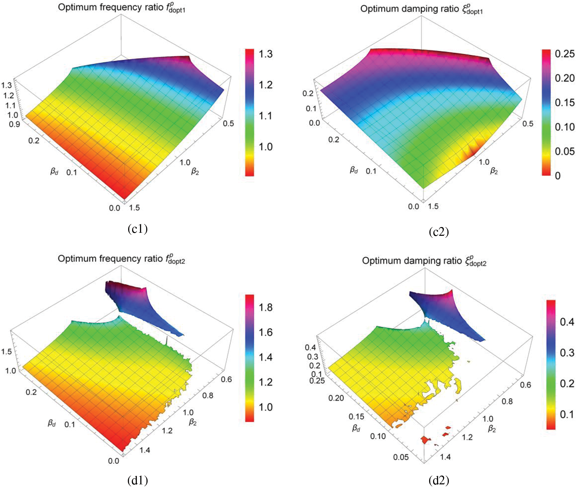
Figure 9: Three-dimensional graphs of optimum solutions
Figure 10: The curves of the optimum solutions (
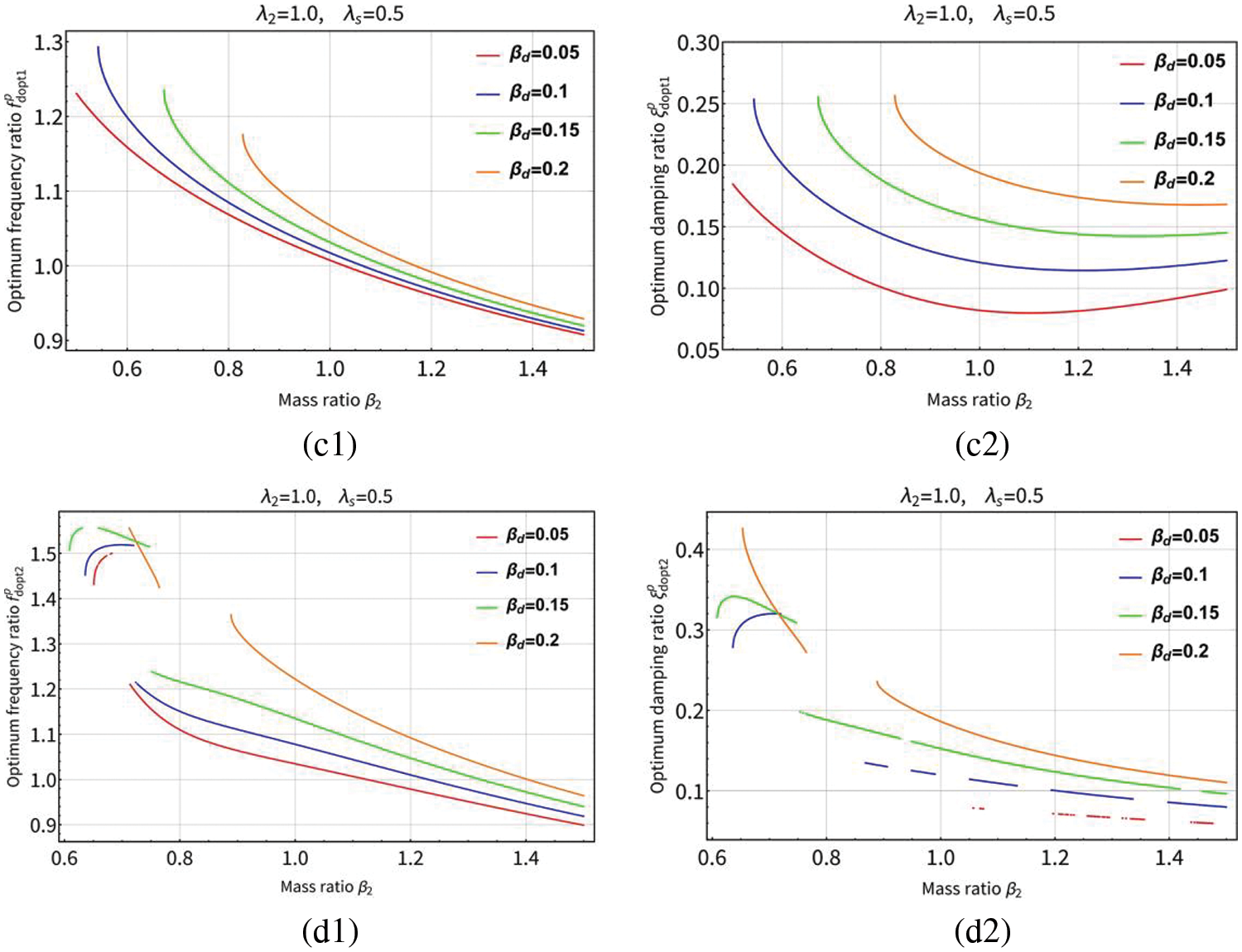
Figure 11: The curves of the optimum solutions (
In Figs. 8(a1) and 8(a2), the optimum frequency ratio
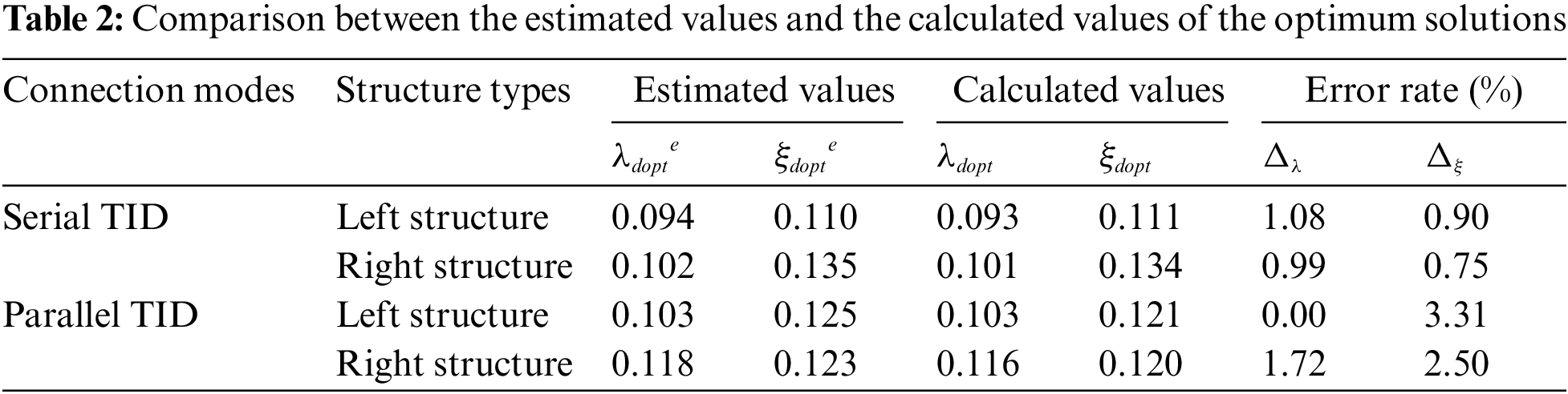
Under parallel TID coupling, it can be seen from Fig. 9 that the
4.2.2 Influence of Stiffness Ratios
Figs. 12 and 13 are three-dimensional graphs of optimum solutions

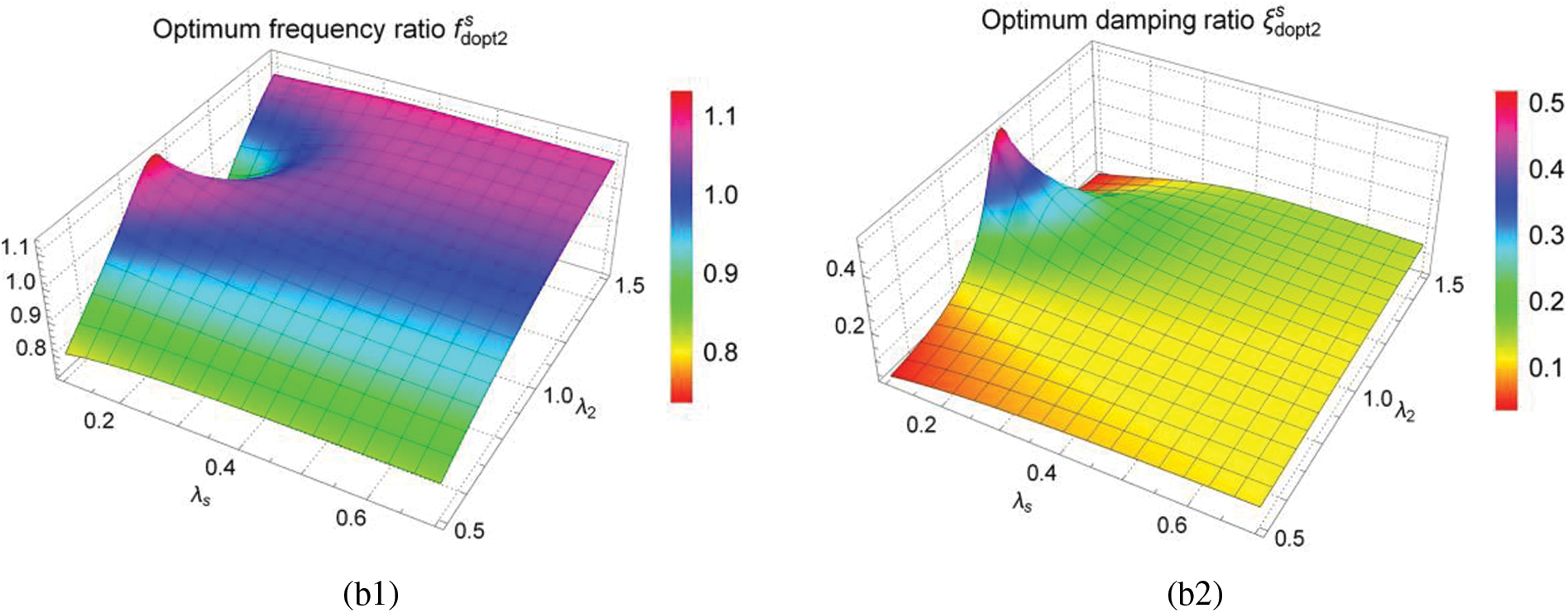
Figure 12: Three-dimensional graphs of the optimum solutions
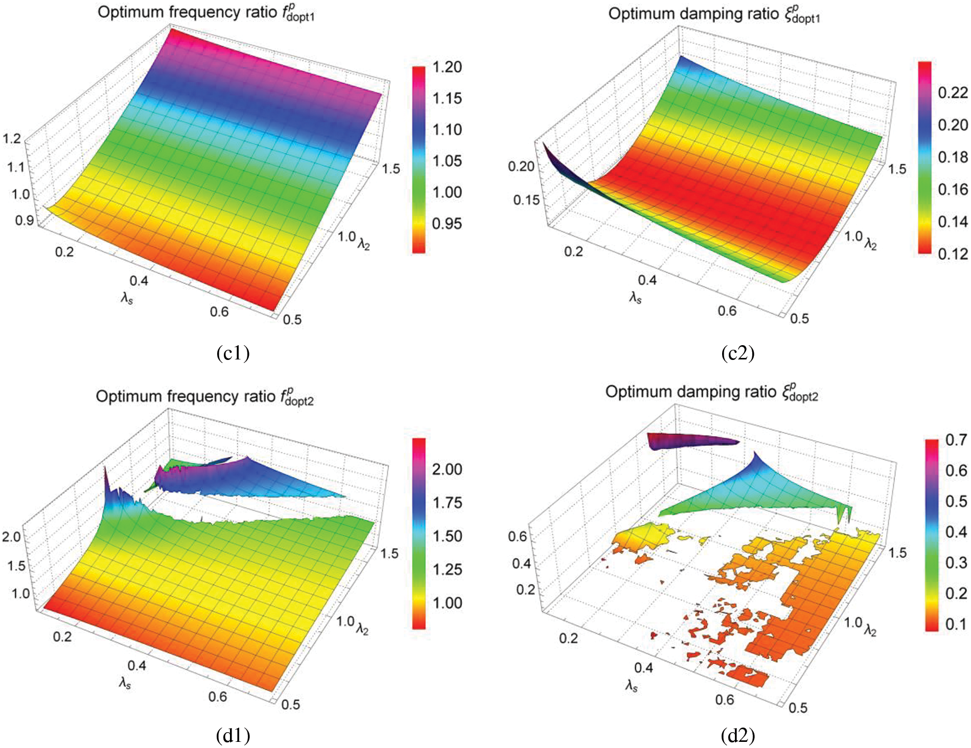
Figure 13: Three-dimensional graphs of the optimum solutions

Figure 14: The curves of the optimum solutions (
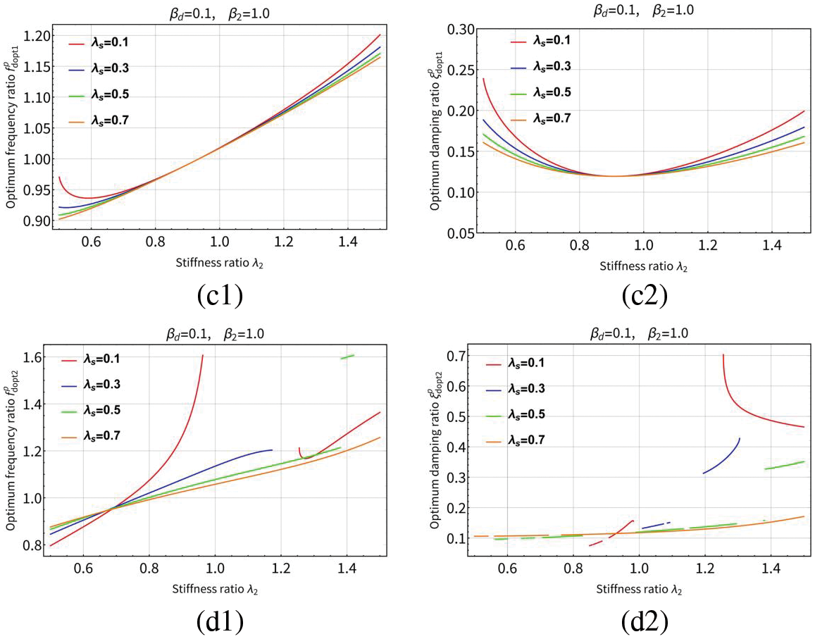
Figure 15: The curves of the optimum solutions (
For the adjacent buildings coupled by serial TID, it can be seen from Figs. 12, 14(a1) and 14(a2) that the optimum frequency ratio
For adjacent buildings with parallel TID coupling, it can be seen from Figs. 13, 15(c1) and 15(c2) that the optimum frequency ratio
After parameter analysis, we introduce classic tuned mass damper (TMD) into the earthquake resistance of adjacent building structures, and analyze its vibration control performance. Under the condition that all the conditions of the specified structure are unchanged, the vibration control performance of two types of TID and TMD are compared.
Fig. 16 shows the damping model of adjacent buildings coupled with TMD, which is the same as the definition in Section 3.1. It is defined that the structure on the left side is the left structure and the structure on the right side is the right structure. The mass, damping and stiffness of TMD are
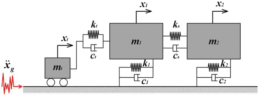
Figure 16: The damping system of adjacent buildings coupled with classic TMD
According to the principle of force balance, the dynamic equilibrium equations are:
Using Laplace transform to make dimensionless, and after finishing, get:
where
Same as the steps in Section 3, the optimization results obtained by H2 optimization method are as follows:
(1) Left structure
where
Similarly, for the classic TMD, there are:
(2) Right structure
where
In order to compare the damping performance of two types of TID and classic TMD, this section adopts the parameters determined in Section 4.1, namely
5.2 Comparison of Vibration Control Effect
In the previous analysis, the values of relevant parameters have been determined as follows:

Figure 17: Normalized displacement graphs of the left structure and right structure of adjacent buildings with different types of dampers (
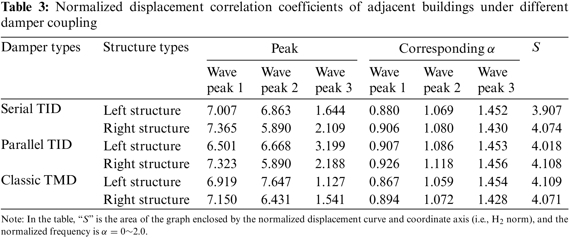
As can be seen from Fig. 17, the similarity of normalized displacement curves under different conditions is high, and there are three peaks. According to the observation of Fig. 17a, compared with the highest point of the whole curve, the parallel TID value is the smallest; according to the observation of Fig. 17b, compared with the highest point of the whole curve, the classic TMD value is the smallest. The above results show that when damping adjacent buildings, the best control effect can be achieved by selecting parallel TID for the left structure and classic TMD for the right structure. For further comparison, the relevant data of Figs. 17a and 17b are summarized in Table 3. It can be seen from the table that compared with the highest point of displacement curve, the left structure is smaller than the right structure for the adjacent buildings coupled by serial and parallel TIDs, which indicates that TID has better vibration control effect for the left structure. However, for the adjacent buildings coupled with classic TMD, the highest point of the displacement curve of the left structure is larger than that of the right structure, which indicates that the classic TMD has a better damping effect on the right structure. From the results given in Table 3, it can be seen that if the size of the area S (i.e., H2 norm) enclosed by the displacement curve and the coordinate axis in the normalized frequency range of 0~2.0 is taken as the basis (hereinafter referred to as area S for convenience of analysis), the serial TID has a better vibration control effect for the left structure, and the classic TMD has a better vibration control effect for the right structure.
As far as the damping effect of TID is concerned, only the specific case of mass ratio

Figure 18: Three-dimensional graphs of normalized displacement when the mass ratio

Figure 19: Considering the different values of mass ratio
It can be seen from Fig. 19a that increasing the mass ratio
The above analysis results show that when the mass of the damper is small compared with that of the left structure (
5.3 Robustness Performance Analysis
Optimization parameters in practical engineering often change. In order to make adjacent buildings achieve more robust vibration control effect, it is necessary to analyze their robustness. Fig. 20 is the robustness analysis curve of the left structure and the right structure under the coupling of serial TID and parallel TID. The optimum frequency ratio

Figure 20: Robustness performance analysis curves of left structure and right structure of adjacent buildings under the coupling of serial TID and parallel TID: (a) Serial TID is coupled with the left structure; (b) Serial TID is coupled with the right structure; (c) Parallel TID is coupled with the left structure; (d) Parallel TID is coupled with the right structure (
As shown in Fig. 20, slightly change the damping ratio the value of
To further determine the size of the change, the detailed drawing of Fig. 20d is shown in Fig. 21. It can be seen from the figure that the right structure in adjacent buildings under the coupling of parallel TIDs is extremely sensitive to the reduction of frequency ratio

Figure 21: Robust performance analysis curve of the right structure of adjacent buildings under the coupling of parallel TID
6.1 Vibration Control Performance
In the foregoing analysis, we assume that the external excitation is white noise excitation with evenly distributed energy at all frequencies, but the ground motion caused by earthquake is actually not ideal white noise [35]. Therefore, it is necessary to simulate and verify the seismic performance of adjacent buildings under the coupling of serial TID and parallel TID. Taking two ten-story frame structures as an example, the relevant parameters of the adjacent building structures are:
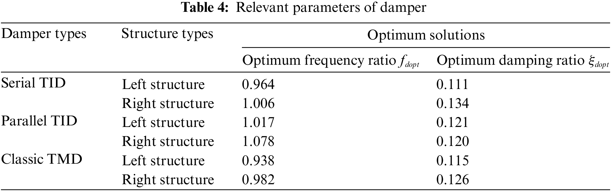
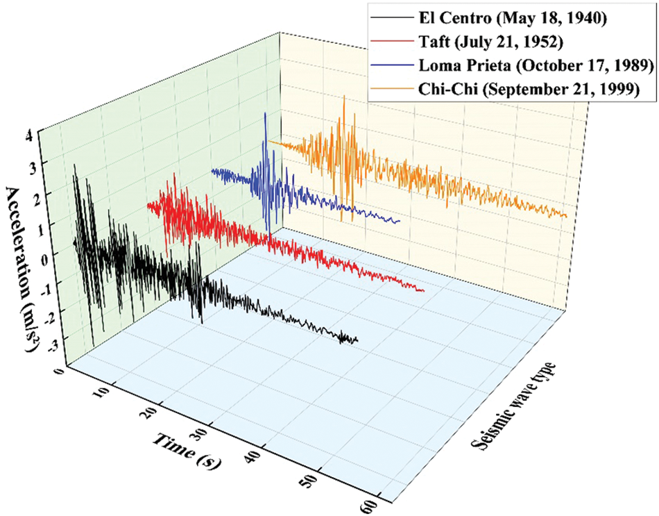
Figure 22: Acceleration time history curves of four types of seismic waves

Figure 23: Displacement time history graphs of the left structure under four types of seismic waves excitation

Figure 24: Displacement time history graphs of the right structure under four types of seismic waves excitation
It can be seen from Fig. 23 that under the excitation of different types of seismic waves, compared with the displacement of the left structure in the uncontrolled state, the three dampers have good damping effects in the whole range. Comparing the displacement of three dampers, it is found that the displacement of classical TMD is slightly larger than that of serial or parallel TID. In order to make a more accurate comparison, the peak and root mean square values of the displacement of the left structure coupled with three different types of dampers are summarized, as shown in Table 5. It can be seen from Table 5 that, compared with the peak displacement in uncontrolled state, the peak control effect of the serial TID is at least 10.1% and at most 47.8%; the peak control effect of parallel TID is at least 9.5% and at most 45.9%; the peak control effect of classic TMD is at least 2.8% and at most 42.3%. As for the control effect of RMS, the control effect of serial TID is at least 21.6% and at most 53.2%; the control effect of parallel TID is at least 18.6% and at most 51.3%, the control effect of classical TMD is at least 14.7% and at most 49.4%. It can be found that under the vibration control of the above model, the root mean square control effect is often greater than the peak damping ratio. The above results show that for the left structure coupled with three types of dampers, all of them can achieve good damping effect, among which the serial TID has the best damping effect, the parallel TID is the second, and the classic TMD is the last.
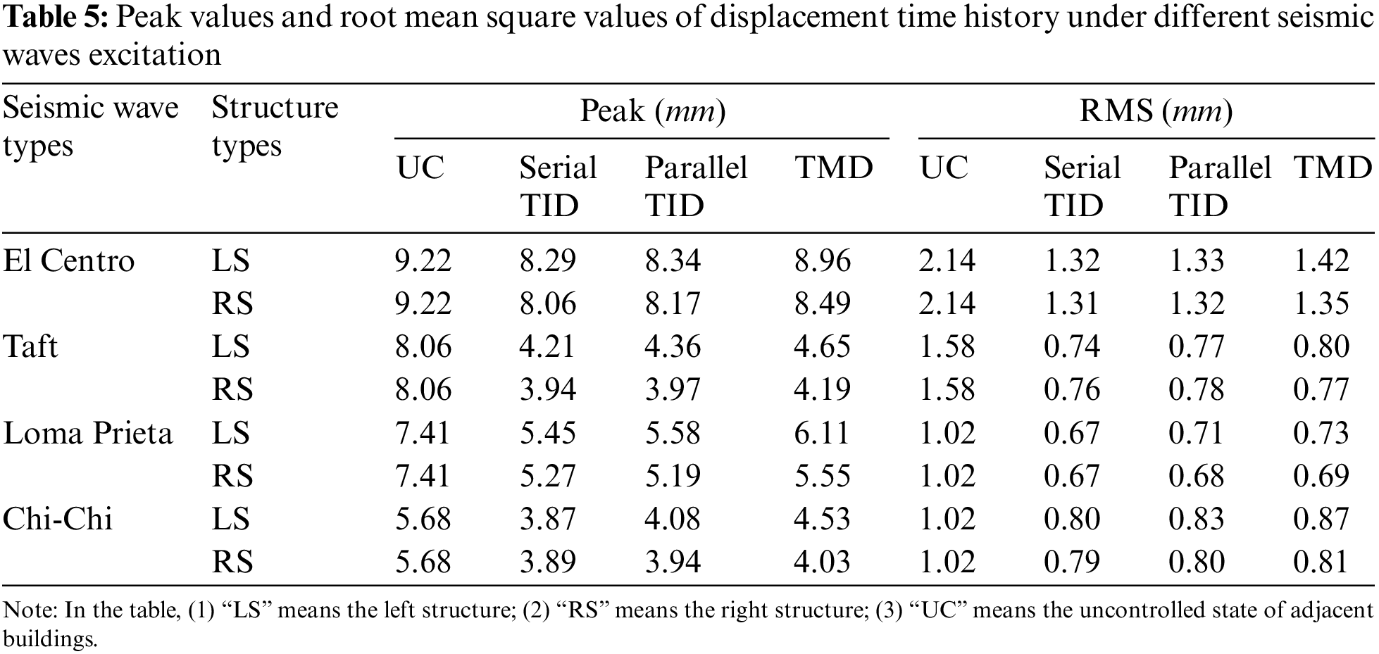
It can be seen from Fig. 24 that, similar to the left structure, under the excitation of different types of seismic waves, compared with the displacement of the right structure in the uncontrolled state, the three dampers have good damping effects in the whole range. Comparing the displacement of three dampers, it is found that the displacement of classic TMD is slightly larger than that of serial or parallel TID. It can be seen from Table 5 that, for the right structure, compared with the peak displacement in uncontrolled state, the peak control effect of the serial TID is at least 12.6% and at most 51.1%; the peak control effect of parallel TID is at least 11.4% and at most 50.7%; the peak control effect of classic TMD is at least 7.9% and at most 48.0%. As for the control effect of RMS, the control effect of serial TID is at least 22.6% and at most 51.9%; the control effect of parallel TID is at least 21.6% and at most 50.6%, the control effect of classical TMD is at least 20.6% and at most 51.3%. The above results show that for the right structure coupled with three types of dampers, all of them can achieve good damping effect, among which the serial TID has the best damping effect, the parallel TID is the second, and the classic TMD is the last. In addition, it can be found that the right structure can achieve better damping effect than the left structure when the adjacent buildings are coupled with the same damper.
As mentioned in Section 2.2, installing the roller generator inside the inerter device can collect part of the vibration energy during the earthquake and make use of it. Therefore, in this paper, we connect the left structure with the TID to collect the vibration energy of the building structure. Based on the fact that the power consumption of the external resistor is basically equivalent to that of the TID buffer element, the power calculation formula can be expressed as

Figure 25: Energy collection graphs of the left structure under four types of seismic waves excitation
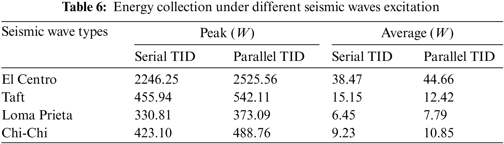
It can be seen from Table 6 that the left structure under the excitation of El Centro seismic wave has a remarkable energy collection effect, with its power peak value reaching 2525.56 W and power root mean square value reaching 44.66 W. According to the calculation, the energy collected in the whole period of El Centro seismic wave is 1.44 × 10⁵ J. Compared with the classical TMD, it is known from the analysis results in Section 5.2 that the vibration reduction effect of TID is better than that of the classic TMD. At the same time, TID has the advantage of collecting energy, when an earthquake occurs, it can store part of the energy for the structure itself, and use it according to the actual situation. Therefore, in real life, when the economic cost is similar, compared with the classic TMD, TID should be preferred to achieve the dual effects of structural vibration control and energy collection.
In this paper, two types of tuned inerter damper (TID) adjacent building damping systems composed of springs, inerters and dampers in serial or in parallel were proposed. H2 norm criterion was adopted to optimize and adjust the damping system of adjacent buildings, so that the system had the best damping performance under the random excitation of white noise. The parameter analysis, frequency response analysis, robustness analysis, time history response analysis and energy collection analysis of the system were carried out successively. Through the above analysis, the following conclusions are drawn:
(1) As for the H2 norm optimization results of adjacent buildings, when considering the value of mass ratios
(2) When studying the displacement frequency response of adjacent buildings, it was found that when
(3) As for the seismic robustness of adjacent building structures under TID coupling, the normalized displacement was less affected by the optimum damping ratio
(4) The time history analysis results of adjacent buildings excited by four types of seismic waves showed that all three types of dampers could achieve a good damping effect, among which the serial TID was the best, the parallel TID was the second, and the classic TMD was the last. In addition, for adjacent buildings coupled with the same damper, the right structure could often achieve a better damping effect than the left structure. According to the time history analysis of energy collection of adjacent buildings excited by four types of seismic waves, it was found that the left structure excited by El Centro seismic waves had the best energy collection effect, with its instantaneous peak power reaching 2525.56 W and the root mean square power reaching 44.66 W in the whole period. According to the calculation, the energy collected in the whole period of El Centro seismic wave was 1.44 × 10⁵ J. In addition, when collecting the vibration energy of adjacent building structures under earthquake excitation, it was found that parallel TID should be given priority.
Based on the above analysis results, in general, the proposed TIDs with different connection modes had significant effects on the vibration control of adjacent buildings, and their performance was superior to that of classic TMDs. In addition, this type of TID also had the function of energy collection, which further expands its application range. The research results of this article could provide some reference significance for the vibration control research of adjacent buildings, however, the application of TIDs proposed in this paper in practical engineering needs further research and demonstration to achieve better vibration control effects.
Acknowledgement: The authors are very grateful to the editors and all anonymous reviewers for their insightful comments.
Funding Statement: This research was funded by the Natural Science Research Project of Higher Education Institutions in Anhui Province (Grant No. 2022AH040045), the Anhui Provincial Natural Science Foundation (Grant No. 2008085QE245), the Project of Science and Technology Plan of Department of Housing and Urban-Rural Development of Anhui Province (Grant No. 2021-YF22).
Author Contributions: The authors confirm contribution to the paper as follows: study conception and design: Xiaofang Kang and Jian Wu; data collection: Jian Wu and Xinqi Wang; analysis and interpretation of results: Jian Wu and Shancheng Lei; draft manuscript preparation: Xiaofang Kang and Jian Wu. All authors reviewed the results and approved the final version of the manuscript.
Availability of Data and Materials: No new data and materials were created or analyzed in this study. Data and material sharing are not applicable for this article.
Conflicts of Interest: The authors declare that they have no conflicts of interest to report regarding the present study.
References
1. Lee, C. H., Chen, Y. C., Wang, F. C. (2015). Earthquake suppression for a scale building model employing inclined inerter. IEEE/SICE International Symposium on System Integration (SII), pp. 828–833. Nagoya, Japan. [Google Scholar]
2. Luo, Y. (2017). Study on parameter optimization of structure vibration control with electromagnetic energy collecting tuned mass damper. Hunan University of Science and Technology, China. [Google Scholar]
3. Housner, G. W., Bergman, L. A., Caughey, T. K., Chassiakos, A. G., Claus, R. O. et al. (1997). Structural control: Past, present, and future. Journal of Engineering Mechanics, 123, 897–971. [Google Scholar]
4. Soong, T., Spencer, B. F. (2002). Supplemental energy dissipation: State-of-the-art and state-of-the-practice. Engineering Structures, 24(3), 243–259. [Google Scholar]
5. Frahm, H. (1911). Device for damping vibrations of bodies. US989958, USA. [Google Scholar]
6. Kareem, A., Kijewski, T., Tamura, Y. (1999). Mitigation of motions of tall buildings with specific examples of recent applications. Wind and Structures, 2(3), 201–251. [Google Scholar]
7. Zuo, H., Bi, K., Hao, H., Ma, R. (2021). Influences of ground motion parameters and structural damping on the optimum design of inerter-based tuned mass dampers. Engineering Structures, 227, 111422. [Google Scholar]
8. Zhu, H., Li, Y., Shen, W., Zhu, S. (2019). Mechanical and energy-harvesting model for electromagnetic inertial mass dampers. Mechanical Systems and Signal Processing, 120, 203–220. [Google Scholar]
9. Nakamura, Y., Fukukita, A., Tamura, K., Yamazaki, I., Matsuoka, T. et al. (2014). Seismic response control using electromagnetic inertial mass dampers. Earthquake Engineering & Structural Dynamics, 43, 507–527. [Google Scholar]
10. Ma, R., Bi, K., Hao, H. (2019). A novel rotational inertia damper for heave motion suppression of semisubmersible platform in the shallow sea. Structural Control & Health Monitoring, 26(7), e2368. [Google Scholar]
11. Ma, R., Bi, K., Hao, H. (2020). Using inerter-based control device to mitigate heave and pitch motions of semi-submersible platform in the shallow sea. Engineering Structures, 207, 110248. [Google Scholar]
12. Garrido, H., Curadelli, O., Ambrosini, D. (2013). Improvement of tuned mass damper by using rotational inertia through tuned viscous mass damper. Engineering Structures, 56, 2149–2153. [Google Scholar]
13. Javidialesaadi, A., Wierschem, N. E. (2018). Optimal design of rotational inertial double tuned mass dampers under random excitation. Engineering Structures, 165, 412–421. [Google Scholar]
14. Li, Y., Li, S., Chen, Z. (2020). Optimization and wind-induced vibration suppression of rotational inertia double tuned mass damper. Journal of Vibration Engineering, 33(2), 295–303. [Google Scholar]
15. Marian, L., Giaralis, A. (2014). Optimal design of a novel tuned mass-damper-inerter (TMDI) passive vibration control configuration for stochastically support-excited structural systems. Probabilistic Engineering Mechanics, 38, 156–164. [Google Scholar]
16. Cao, L., Li, C. (2019). Tuned tandem mass dampers-inerters with broadband high effectiveness for structures under white noise base excitations. Structural Control & Health Monitoring, 26(4), e2319. [Google Scholar]
17. Zhao, X., Li, C., Cao, L. (2022). Control performance of structure-NFVD-TTMDI. Journal of Vibration Engineering, 35(1), 55–63. [Google Scholar]
18. Zhao, Z., Zhang, R., Jiang, Y., Pan, C. (2019). A tuned liquid inerter system for vibration control. International Journal of Mechanical Sciences, 164, 105171. [Google Scholar]
19. Lazar, I., Neild, S., Wagg, D. (2014). Using an inerter-based device for structural vibration suppression. Earthquake Engineering & Structural Dynamics, 43(8), 1129–1147. [Google Scholar]
20. Lazar, I., Neild, S., Wagg, D. (2016). Vibration suppression of cables using tuned inerter dampers. Engineering Structures, 122, 62–71. [Google Scholar]
21. Sun, L., Hong, D., Chen, L. (2017). Cables interconnected with tuned inerter damper for vibration mitigation. Engineering Structures, 151, 57–67. [Google Scholar]
22. Deastra, P., Wagg, D., Sims, N., Akbar, M. (2020). Tuned inerter dampers with linear hysteretic damping. Earthquake Engineering & Structural Dynamics, 49(12), 1216–1235. [Google Scholar]
23. Shi, B., Yang, J., Jiang, J. Z. (2022). Tuning methods for tuned inerter dampers coupled to nonlinear primary systems. Nonlinear Dynamics, 107, 1663–1685. [Google Scholar]
24. Bin, T., Wang, X., Fang, H., Wang, W. (2020). Analysis of mitigating performance of tuned inerter mass dampers. Noise and Vibration Control, 40(4), 223–226. [Google Scholar]
25. De Domenico, D., Ricciardi, G., Zhang, R. (2020). Optimal design and seismic performance of tuned fluid inerter applied to structures with friction pendulum isolators. Soil Dynamics and Earthquake Engineering, 132, 106099. [Google Scholar]
26. de Domenico, D., Deastra, P., Ricciardi, G., Sims, N. D., Wagg, D. J. (2019). Novel fluid inerter based tuned mass dampers for optimised structural control of base-isolated buildings. Journal of the Franklin Institute-Engineering and Applied Mathematics, 356(14), 7626–7649. [Google Scholar]
27. Liang, Q., Li, L. (2020). Optimal design for a novel inerter-based clutching tuned mass damper system. Journal of Vibration and Control, 26(21–22), 2050–2059. [Google Scholar]
28. Smith, M. C. (2002). Synthesis of mechanical networks: The inerter. IEEE Transactions on Automatic Control, 47, 1648–1662. [Google Scholar]
29. Hwang, J. S., Kim, J., Kim, Y. M. (2007). Rotational inertia dampers with toggle bracing for vibration control of a building structure. Engineering Structures, 29(6), 1201–1208. [Google Scholar]
30. Swift, S. J., Smith, M. C., Glover, A. R., Papageorgiou, C., Gartner, B. et al. (2013). Design and modelling of a fluid inerter. International Journal of Control, 86(11), 2035–2051. [Google Scholar]
31. De Domenico, D., Ricciardi, G. (2018). An enhanced base isolation system equipped with optimal tuned mass damper inerter (TMDI). Earthquake Engineering & Structural Dynamics, 47(5), 1169–1192. [Google Scholar]
32. Javidialesaadi, A., Wierschem, N. E. (2018). Three-element vibration absorber-inerter for passive control of single-degree-of-freedom structures. Journal of Vibration and Acoustics-Transactions of the ASME, 140(6), 061007. [Google Scholar]
33. Chen, M. Z. Q., Papageorgiou, C., Scheibe, F., Wang, F. C., Smith, M. C. (2009). The missing mechanical circuit element. IEEE Circuits and Systems Magazine, 9, 10–26. [Google Scholar]
34. Papageorgiou, C., Houghton, N. E., Smith, M. C. (2009). Experimental testing and analysis of inerter devices. Journal of Dynamic Systems Measurement and Control-Transactions of the ASME, 131, 011001. [Google Scholar]
35. Qian, F., Luo, Y., Sun, H., Tai, W., Zuo, L. (2019). Optimal tuned inerter dampers for performance enhancement of vibration isolation. Engineering Structures, 198, 109464. [Google Scholar]
36. Ikago, K., Saito, K., Inoue, N. (2012). Seismic control of single-degree-of-freedom structure using tuned viscous mass damper. Earthquake Engineering & Structural Dynamics, 41(3), 453–474. [Google Scholar]
37. Dai, J., Xu, Z., Gai, P., Hu, Z. (2021). Optimal design of tuned mass damper inerter with a Maxwell element for mitigating the vortex-induced vibration in bridges. Mechanical Systems and Signal Processing, 148, 107180. [Google Scholar]
38. Dai, J., Xu, Z., Gai, P. (2019). Tuned mass-damper-inerter control of wind-induced vibration of flexible structures based on inerter location. Engineering Structures, 199, 109585. [Google Scholar]
39. Sun, H., Zuo, L., Wang, X., Peng, J., Wang, W. (2019). Exact H2 optimal solutions to inerter-based isolation systems for building structures. Structural Control & Health Monitoring, 26(6), e2357. [Google Scholar]
40. Jangid, R. S. (2021). Optimum tuned inerter damper for base-isolated structures. Journal of Vibration Engineering & Technologies, 9, 1483–1497. [Google Scholar]
41. Gonzalez-Buelga, A., Clare, L. R., Neild, S. A., Jiang, J. Z., Inman, D. J. (2015). An electromagnetic inerter-based vibration suppression device. Smart Materials and Structures, 24, 055015. [Google Scholar]
42. Shen, W., Niyitangamahoro, A., Feng, Z., Zhu, H. (2019). Tuned inerter dampers for civil structures subjected to earthquake ground motions: Optimum design and seismic performance. Engineering Structures, 198, 109470. [Google Scholar]
43. Crandall, S. H., Mark, W. D. (1963). Random vibration in mechanical systems. USA: Academic Press. [Google Scholar]
44. Asami, T., Nishihara, O., Baz, A. M. (2002). Analytical solutions to H∞ and H2 optimization of dynamic vibration absorbers attached to damped linear systems. Journal of Vibration and Acoustics-Transactions of the ASME, 124(2), 284–295. [Google Scholar]
45. Palacios-Quiñonero, F., Rubió-Massegú, J., Rossell, J. M., Karimi, H. R. (2019). Design of inerter-based multi-actuator systems for vibration control of adjacent structures. Journal of the Franklin Institute, 356(14), 7785–7809. [Google Scholar]
46. Djerouni, S., Elias, S., Abdeddaim, M., Rupakhety, R. (2022). Optimal design and performance assessment of multiple tuned mass damper inerters to mitigate seismic pounding of adjacent buildings. Journal of Building Engineering, 48, 103994. [Google Scholar]
47. Luo, Y., Sun, H., Wang, X. (2019). The H2 parametric optimization and structural vibration suppression of electromagnetic tuned mass-inerter dampers. Engineering Mechanics, 36(4), 89–99. [Google Scholar]
48. Sun, H., Luo, Y., Wang, X., Yu, J., Peng, J. (2018). Parametric optimization and vibration control of electromagnetic tuned mass-inerter dampers for the structures. Journal of Shenyang Jianzhu University (Natural Science), 34(3), 410–418. [Google Scholar]
49. Rana, R., Soong, T. T. (1998). Parametric study and simplified design of tuned mass dampers. Engineering Structures, 20(3), 193–204. [Google Scholar]
50. Luo, Y., Sun, H., Wang, X. (2018). H2 parameters optimization and vibration reduction analysis of electromagnetic tuned mass damper. Journal of Vibration Engineering, 31(3), 529–538. [Google Scholar]
Appendix A. The numerator and denominator coefficients of Eq. (7) are as follows:
Appendix B. The numerator coefficient of Eq. (8) is as follows:
Appendix C. The numerator and denominator coefficients of Eq. (9) are as follows:
Appendix D. The numerator coefficient of Eq. (10) is as follows:
Appendix E. Using the Residue Theorem, the evaluation index
where
Appendix F. In Eq. (12), the specific forms of
Appendix G. In Eq. (13), the specific forms of
Appendix H. In Eq. (14), the specific forms of
Appendix I. In Eq. (15), the specific forms of
Appendix J. The specific forms of
Appendix K. The optimization results Eq. (26) can be obtained by solving Eq. (24), where the specific form of polynomial
Here, it is necessary to point out the calculation process of the optimum solutions
Substituting Eqs. (I1), (I2), (20), (J1)–(J10) and (K1)–(K5) into Eq. (26), the calculated result is:
In the above Equation,
Appendix L. In Eq. (31), the specific forms of
Appendix M. In Eq. (33), the specific forms of
Cite This Article
 Copyright © 2024 The Author(s). Published by Tech Science Press.
This work is licensed under a Creative Commons Attribution 4.0 International License , which permits unrestricted use, distribution, and reproduction in any medium, provided the original work is properly cited.
 Downloads
 Citation Tools