Time-Domain Analysis of Body Freedom Flutter Based on 6DOF Equation

1  Introduction

Modern vehicles use new airfoils, wingtips, high-lift devices, and flow control methods to improve aerodynamic efficiency and lightweight structures to reduce vehicle weight. With the development of aerodynamics, structural dynamics, and material technology, the shape and internal structure of vehicles are changing dramatically. Various unconventional layouts also bring new stability problems and different types of flutter. The wing design towards lightweight and flexible high aspect ratio makes the 1st bending mode frequency low. The low-order bending mode can be coupled with the rigid body short-period mode to produce a new type of flutter-body freedom flutter (BFF) [1–4].

In the 1940s, the occurrence of body freedom flutter in a vehicle with a high aspect ratio and tailless flying wings was discovered. In the 1980s, Schweiger et al. [5] explained the mechanism of the occurrence of body freedom flutter in the flexible vehicle. Since then, a lot of research has been conducted on the body freedom flutter. In 2010, the Air Force Research Laboratory (AFRL), in conjunction with Lockheed Martin Aeronautics (LM Aero) Company, proposed a program to establish the X-56A Multi-utility technology testbed (MUTT). One of its objectives was to systematically study the body freedom flutter phenomenon of flying wing vehicles and develop Integrated Flight and Aeroelastic Control (IFAC) technology [6–8]. Richards et al. [9] constructed a high-aspect-ratio vehicle with a variable center of gravity and pitch inertia and calculated its body freedom flutter characteristics by a simplified aerodynamic model. The calculation results showed that the pitching angular velocity was a major factor in affecting body freedom flutter and suggested that the occurrence of body freedom flutter could be avoided by increasing the pitch inertia, reducing the fuselage weight, and lowering the center of gravity position. Guo et al. [10] investigated the effectiveness of a passive gust alleviation device (PGAD) installed at the wing tip in a flying wing layout for body freedom flutter suppression. The results showed that the PGAD could reduce the gust-induced wing root bending moment by 16% and increase the BFF speed of the flying wing aircraft by 4.2%. Huang et al. [11] combined the autoregressive coefficients with the Jury stability criterion to develop a body freedom flutter prediction model. The applicability of the autoregressive sliding average method in predicting the flutter boundary of the wing model was verified. Lei et al. [12] used CFD/CSD time-domain coupling method, combined with the variable stiffness technique, to perform body freedom flutter analysis and validation with wind tunnel tests.

With the development of active control techniques, research on body freedom flutter has begun to focus on active flutter suppression. For example, the University of Minnesota established a lower order reduced-order model based on the developed CFD/CSD coupling calculation model of body freedom flutter and then studied active flutter suppression technology [13,14].

For the calculation and analysis of body freedom flutter, most researchers now use Nastran commercial software. The unsteady aerodynamic force prediction adopts the double-lattice method or the reduced-order aerodynamic model. The research on flutter calculation methods based on high-precision CFD/CSD coupling is still less.

The main purpose of this paper is to establish a high-precision BFF prediction method by utilizing the 6DOF equation instead of the rigid mode method. The primary differences between the two approaches involve the coordinate frames used in deriving the equations of motion. In the rigid mode method, all the DOFs, as well as aerodynamic forces and moments, are defined in the inertial reference frame, while in 6DOF equations, the motion variables, forces, and moments are always defined in a body-reference frame. The latter approach, for example, yields time-invariant vehicle-mass properties (for rigid vehicles) and is compatible with onboard sensor measurements employed in the flight-control systems as well as piloted simulations. It can more accurately and intuitively reflect the change of vehicle attitude in the BFF calculation and assist the design of active flutter suppression control law [15].

In this paper, aiming at the high-precision prediction of BFF, the CFD/CSD/6DOF time-domain coupled simulation method is used to predict the BFF characteristics of a flying wing vehicle. The influences of plunge motion, the center of mass position, and the moment of inertia on the BFF characteristics of the flying wing vehicle and their mechanisms are discussed.

2  Calculation Methods

2.1 CFD Solver

The three-dimensional Euler/RANS equations are considered in this work. The integral form in the moving grid system under the Cartesian coordinate system is

∂∂t∫ΩWdΩ+∮∂Ω(FcM−Fv)dS=0(1)

where the vectors of conservative variables W, convective fluxes FcM, and viscous fluxes Fv are given by

W=[ρρuρvρwρE],FcM=[ρVrρuVr+nxpρvVr+nypρwVr+nzp(ρE+p)Vr+Vtp],Fv=[0nxτxx+nyτxy+nzτxznxτyx+nyτyy+nzτyznxτzx+nyτzy+nzτzznxΘx+nyΘy+nzΘz](2)

In the above expressions, ρ,u,v,w,E denote density, velocity components, and total energy per unit mass, Vr represents the contravariant velocity relative to the grid motion and τij represents the components of the viscous stress tensor.

Additionally, the so-called Geometric Conservation Law (GCL) has to be fulfilled in order to avoid the errors induced by the deformations of the control volume [16]. The integral form of the GCL can be formulated as

∂∂t∬ΩdΩ−∮∂Ωvt⋅ndS=0(3)

with vt being the grid velocity vector.

The cell-centered finite volume method is applied for spatial discretization of Eq. (1). The 5-stage Runge-Kutta time-stepping method with local time stepping technique [17] and the dual time-stepping approach [16] are employed for temporal discretization. The S-A one-equation turbulence model [18] is adopted. The N-S solver is parallelized for higher computational efficiency. This in-house CFD solver has been frequently applied to aerodynamic and aeroelastic calculations [19–22].

2.2 CSD Solver

For linear elastic problems, this paper also adopts the modal method to construct the structural equations of motion:

Mqtt+Gqt+Kq=A(4)

where q, qt, qtt are the generalized displacement, velocity, and acceleration vectors respectively, M, G, K are respectively the generalized mass, damping, and stiffness matrices, and A is the generalized aerodynamic vector. The i-th order generalized aerodynamic vector Ai is calculated by the following equation:

Ai=∯[p(i,j,k,t)+τ(i,j,k,t)]⋅hi(i,j,k)dS(5)

where hi(i,j,k) is the vector of the i-th mode shape of the CFD surfaces grid, obtained by interpolation of the structural mode hi(x,y,z), p and τ are the pressure and viscous stress vectors on the surface of the vehicle calculated from the unsteady CFD results, respectively.

The IPS method is adopted to interpolate the mode values from the structural mesh to the CFD surface grid. A second-order Hybrid Linear Multi-step Scheme (HLMS) using predictor-corrector procedure [20,23] is employed to solve Eq. (4). In [23] HLMS was verified to provide high efficiency, high-order accuracy, strong stability, and simple operation for the computation of fluid-structure interaction.

Considering the first n modes, the instantaneous structural displacement can be calculated by the following equation:

Δr(i,j,k,t)=∑i=1nhi(i,j,k)qi(t)(6)

where Δr(i,j,k,t) is the structural deformation vector of the CFD grid point at time t, qi is the i-th order generalized displacement, and n is the number of modes.

2.3 Rigid Body Motion

The rigid body motion of the vehicle has six degrees of freedom and correspondingly six dynamical equations, where three degrees of freedom describe the translational motion of the center of mass and three degrees of freedom describe the rotation motion around the center of mass. In this paper, the motion equations of the center of mass are established in the ground coordinate system, which can be regarded as an inertial coordinate system, while the rotation equations are established in the body coordinate system.

The motion equations of the center of mass are given by Newton’s laws of motion:

md2xcmgdt2=Fxgmd2ycmgdt2=Fygmd2zcmgdt2=Fzg(7)

where the superscript g denotes the ground coordinate system, (xcmg,ycmg,zcmg) denote the center of mass coordinates, and (Fxg,Fyg,Fzg) are the component forces in three directions.

The rotation of a rigid body around the center of mass is described by the Euler motion equations. For a symmetric vehicle (Ixy=Iyz=0), the Euler motion equations can be simplified as

(Ixxb−IzxbIzzb)dωxbdt=Mxb+(Iyyb−Izzb)ωybωzb+AIyybdωybdt=Myb+(Izzb−Ixxb)ωzbωxb−Izxb(ωxb2−ωzb2)(Izzb−IzxbIxxb)dωzbdt=Mzb+(Ixxb−Iyyb)ωxbωyb+B(8)

where

A=Izxb(ωxbωyb+Mzb−(Iyyb−Ixxb)ωxbωyb−IzxbωybωzbIzzb)B=Izxb(ωybωzb+Mxb−(Izzb−Iyyb)ωybωzb+IzxbωxbωybIxxb)

where the superscript b denotes the body coordinate system, Mb=[Mxb,Myb,Mzb]T denotes the total moment applied to the vehicle in the body coordinate system, ωb=[ωxb,ωyb,ωzb]T is the angular velocity vector and Ixxb, Iyyb, Izzb and Izxb are the moments of inertia, respectively.

The description of the vehicle attitude is then given by the kinematic equation around the center of mass.

{dϕdt=p+tan⁡ θ(q sin⁡ ϕ+r cos⁡ ϕ)dθdt=q cos⁡ ϕ−r sin⁡ ϕdψdt=1cos⁡ θ(q sin⁡ ϕ+r cos⁡ ϕ)(9)

where p, q and r are the components of the angular velocity in three directions, ϕ, θ and ψ are the three Euler angles of the body coordinate system to the ground coordinate system.

The aerodynamic force on the vehicle is obtained by CFD solution, and the velocity and displacement of the center of mass can be obtained by direct integration of Eq. (7). The Eqs. (8) and (9) describe a system of ordinary differential equations, which can be calculated by the 4-stage Runge-Kutta method.

2.4 Dynamic Mesh Generation Method

The original CFD grid is no longer applicable after the surface of the vehicle is deformed. Therefore, it is necessary to generate a new computational grid. We propose a dynamic mesh generation strategy particularly suitable for BFF simulation of free-flying vehicles.

The basic idea of the dynamic mesh generation technique is to keep the far-field boundary stationary and the wall boundary moving with the object motion. The interior mesh is generated by the algebraic method of infinite interpolation.

The dynamic grid point coordinates (subscripted as t) are expressed as

xt=(xr−xs)⋅g+xs(10)

where xs is the initial static grid point, xt denotes the transient coordinate value of this point, and g is the decay rate. Each spatial grid point has a corresponding g value. The key of realizing dynamic grid generation is how to calculate g on each grid point.

In the time-domain BFF computation, the 6DOF equations are used to describe the rigid body motion and the modal method is used to describe the elastic vibration. Next, the automatic dynamic mesh generation technology based on TFI is developed for the modal method and the 6DOF method respectively to realize the efficient calculation of fluid-structure coupling based on a single CFD mesh system.

2.4.1 Dynamic Mesh Strategy of Elastic Deformation

After the structural point mode is interpolated to the CFD surface grid points, the TFI dynamic grid technology is used to further interpolate the surface mode into the entire flow field space.

hi(i,j,k)=hw(i,j,k)⋅g(11)

where hi is the i-th order modal vector of the spatial grid point, hw is the i-th order modal vector of the aerodynamic surface grid point obtained by IPS interpolation from the structural point mode, and g is the decay rate obtained from the following equation:

g=((xf−x)2+(yf−y)2+(zf−z)2(xf−xw)2+(yf−yw)2+(zf−zw)2)(12)

where x, y, z are the grid point coordinate values. The subscript w denotes the vehicle surface grid points and subscript f denotes the grid points of the corresponding far-field boundary.

According to the modal method, the displacement of the spatial grid points can be expressed as

Δre(i,j,k)=∑i=1nhi(i,j,k)⋅qi(13)

where Δre(i,j,k) is the displacement vector of the grid point.

Therefore, the spatial modal interpolation is completed in the pre-processing. The automatic generation of dynamic mesh can be achieved by directly using the spatial modal superposition in the CFD calculation.

2.4.2 Dynamic Mesh Strategy of Rigid Body Motion

Rigid body motion is described by the 6DOF equation. It is possible to use dynamic mesh technology to generate the rigid body displacement interpolation matrix from the object surface to the flow field space. After the rigid body displacement is obtained from the 6DOF calculation, the dynamic mesh can be generated directly by the interpolation matrix.

According to the law of coordinate transformation, the grid point displacement of the vehicle object surface can be obtained:

Δrw(i,j,k)=(Lbg)−1⋅xwg(i,j,k)+xcmg−xsg(i,j,k)(14)

where Δrw(i,j,k) is the displacement vector of the surface grid point. And xsg(i,j,k) represents the initial surface grid point. Therefore, the displacement of grid points in the flow field can be obtained by interpolation:

Δrr(i,j,k)=Δrw(i,j,k)⋅g=[(Lbg)−1⋅xwg(i,j,k)+xcmg−xsg(i,j,k)]⋅g(15)

where Δrr(i,j,k) is the displacement vector of the grid point in the flow field space and Δrw(i,j,k) is the displacement vector of the surface grid point corresponding to the spatial grid point.

That is, to calculate the displacement of the spatial grid point, not only the information of the spatial grid point but also the coordinates of the corresponding surface grid point are required, which increases the difficulty of calculation. To ensure the versatility of the BFF solver, we need to establish the correspondence between the spatial grid points and the surface grid points in the preprocessing program. In the preprocessing, the decay rate g is calculated for each spatial grid point according to Eq. (12), and a matrix B is created to store the surface grid points corresponding to the spatial grid points. That is, the spatial grid point index (i,j,k) corresponding to B(i,j,k) is the surface grid point xwg. In this way, only the grid point index is needed to calculate the displacement of the spatial grid point.

Δrr(i,j,k)=[(Lbg)−1⋅B(i,j,k)+xcmg−xsg(i,j,k)]⋅g(16)

To sum up, considering the rigid body displacement and elastic deformation, the position of the spatial grid point of the flow field at time n can be expressed as

xt(i,j,k)=xs(i,j,k)+Δrr(i,j,k)+Δre(i,j,k)(17)

In this way, based on a single CFD grid system, the dynamic mesh can be automatically generated when the rigid displacement and elastic deformation of the vehicle are known. The interpolation process is completed in the preprocessing process, which can ensure the versatility of the BFF solver for different aerodynamic configurations.

2.5 Static Aeroelastic Trim

The trim of the vehicle refers to solving the angle of attack (AoA) and the deflection angle of each control surface under the condition of given flight state parameters. Generally, the analysis and calculation of fuselage flutter and gust response are based on the static equilibrium state obtained by trimming. The high-aspect-ratio flexible wing will produce large bending and torsional deformation under the action of flight load, and the influence of elastic deformation needs to be considered when trimming.

If only the longitudinal trim problem is considered, and the default engine thrust and drag are in equilibrium, the equilibrium condition of the vehicle in the steady state can be expressed as [24]

L(α,δ,qi)=GMy,CG(α,δ,qi)=0(i=1,2⋅⋅⋅n)Kiiqi=Ai(18)

where L is the lift force on the vehicle. α and δ are the AoA and aileron deflection in the trimming state, G is the gravitational force on the vehicle itself, My,CG is the pitching moment on the center of gravity, Kii is the value of the i-th row and i-th column of the stiffness matrix, qi is the i-th order generalized displacement, Ai is the i-th order generalized aerodynamic force and n is the number of modal orders taken.

Without considering rigid body motion, the CFD/CSD time-domain coupling calculation method is used to perform trimming of the flexible vehicle considering elastic deformation. Within the flutter boundary, the aerodynamic force and aerodynamic configurations considering the influence of static aeroelasticity in this state can be obtained after the CFD/CSD time-domain calculation converges. According to the calculation results for different angles of attack and rudder deflection angles, the angle of attack and the rudder deflection angle at the equilibrium point are obtained by interpolation. The interpolation calculation method is as follows:

{L(α,δ,qi)=Lα⋅(α−α0)+Lδ⋅(δ−δ0)+L0My,CG(α,δ,qi)=Mα⋅(α−α0)+Mδ⋅(δ−δ0)+M0(19)

where α0, δ0, L0 and M0 are the AoA, aileron deflection, lift, and moment at the reference point, respectively, Lα, Mα, Lδ and Mδ are the aerodynamic derivatives.

2.6 Body Freedom Flutter Solver

Based on the static equilibrium state, the 6DOF equation is adopted to describe the rigid body motion, and the modal method is applied to describe the structural elastic vibration. The aerodynamic/structural/rigid body motion control equations are solved in the time domain with loose coupling. A coupled CFD/CSD/6DOF time-domain calculation method for body freedom flutter is developed, combined with the variable stiffness technique [25] to analyze the flutter boundary. The flowchart is shown in Fig. 1.

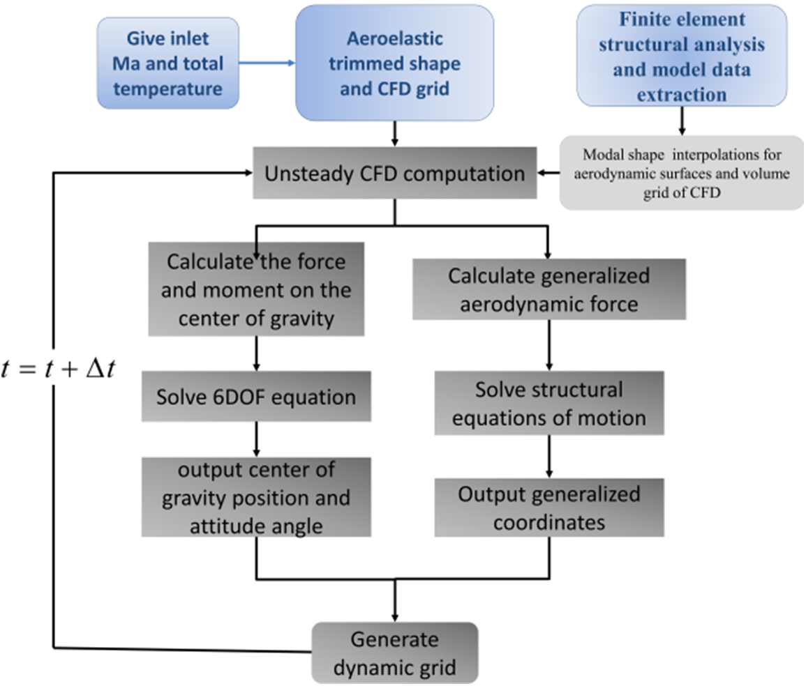
Figure 1: A coupled CFD/CSD/6DOF time-domain calculation method for BFF

In the variable stiffness method, the stiffness of the calculated model is N times the original stiffness. And the flutter dynamic pressure and flutter frequency of the calculated model are QF,m and ωF,m, respectively. Then the flutter dynamic pressure QF,a and the flutter frequency ωF,a of the original stiffness vehicle at a given Mach number on the sea level are expressed as

QF,a=QF,m/NωF,a=ωF,m/N(20)

3  Calculation and Analysis of BFF Characteristics

In this section, the model of the flying wing configuration is used to carry out the numerical calculation of the body freedom flutter based on the CFD/CSD/6DOF coupling method. The simulation results are compared with the calculation results of the modal method and the Nastran software based on the linearization theory.

3.1 Computational Model

The research object is a mid-aspect ratio flying wing vehicle model (Fig. 2). The plane shape of the model refers to X-56a [26,27] and mAEWing1 [14]. These two small UAVs have widely used objects for the body freedom flutter problem. Table 1 lists the detailed parameters of the flying wing model.

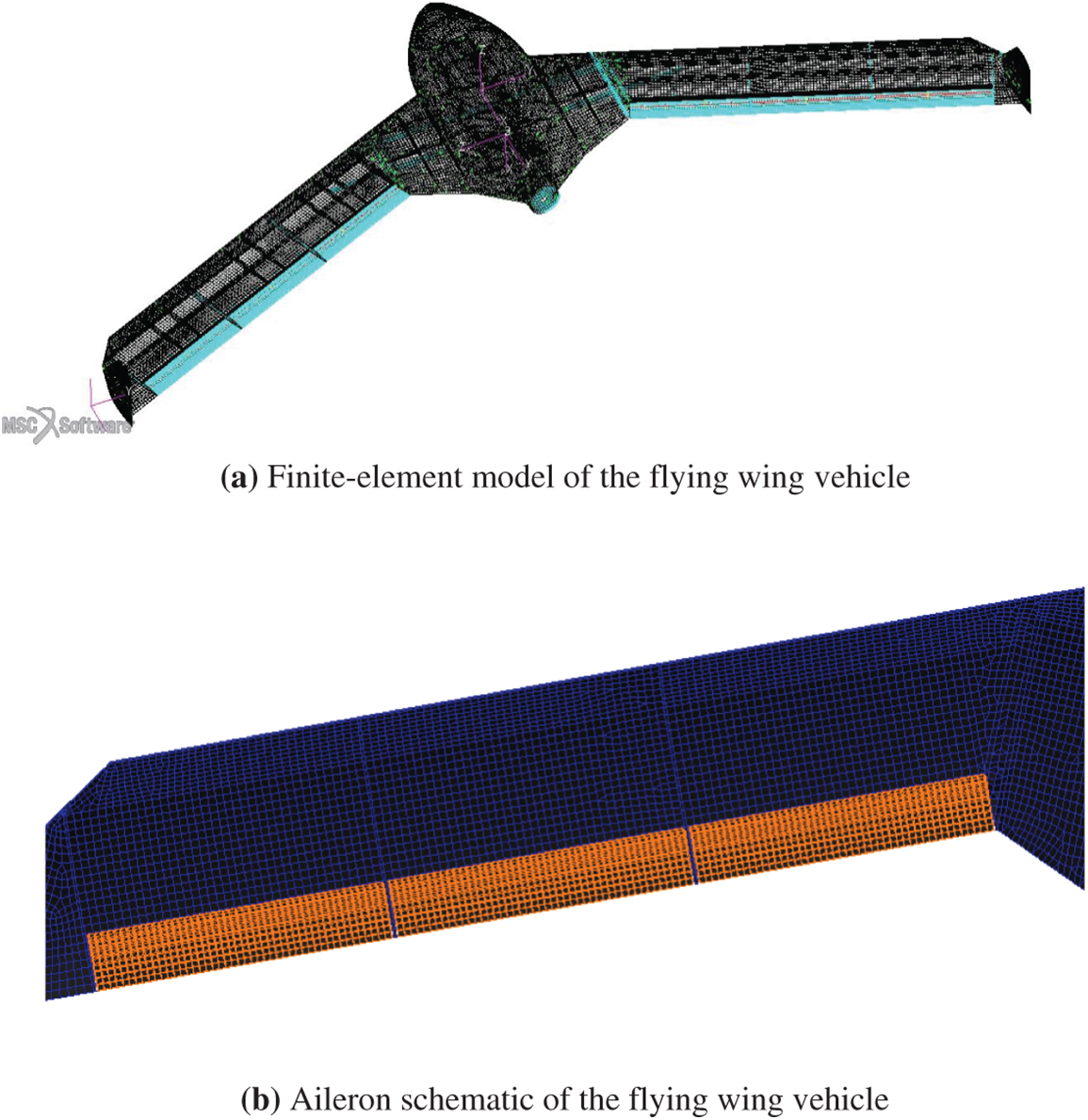
Figure 2: A mid-aspect ratio flying wing vehicle model

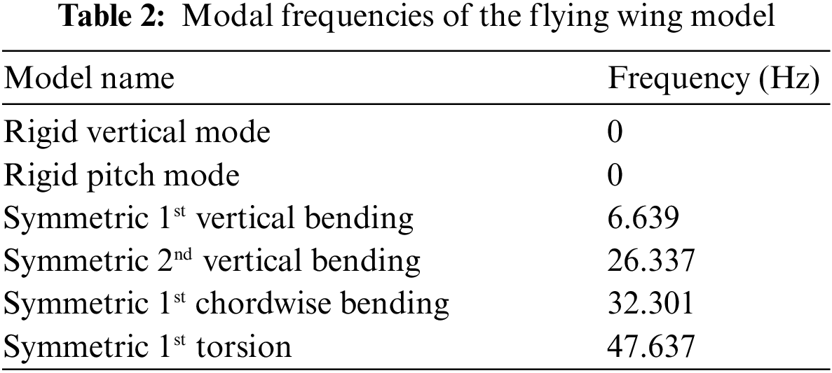
In the research, Nastran software is used to perform natural modal analysis on the UAV model. The first 4 symmetric elastic modes are selected. Fig. 3 shows the corresponding mode shapes. Table 2 gives the modal frequencies of the flying wing model.

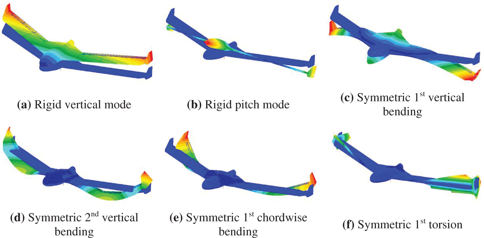
Figure 3: First six symmetric mode shapes of the flying wing model

As shown in Fig. 4, the calculation grid adopts a multi-block structured grid to solve the N-S equation. The grid height of the first layer of the object surface is 1.0×10−5c0, and the number of grids is 1.432 million.

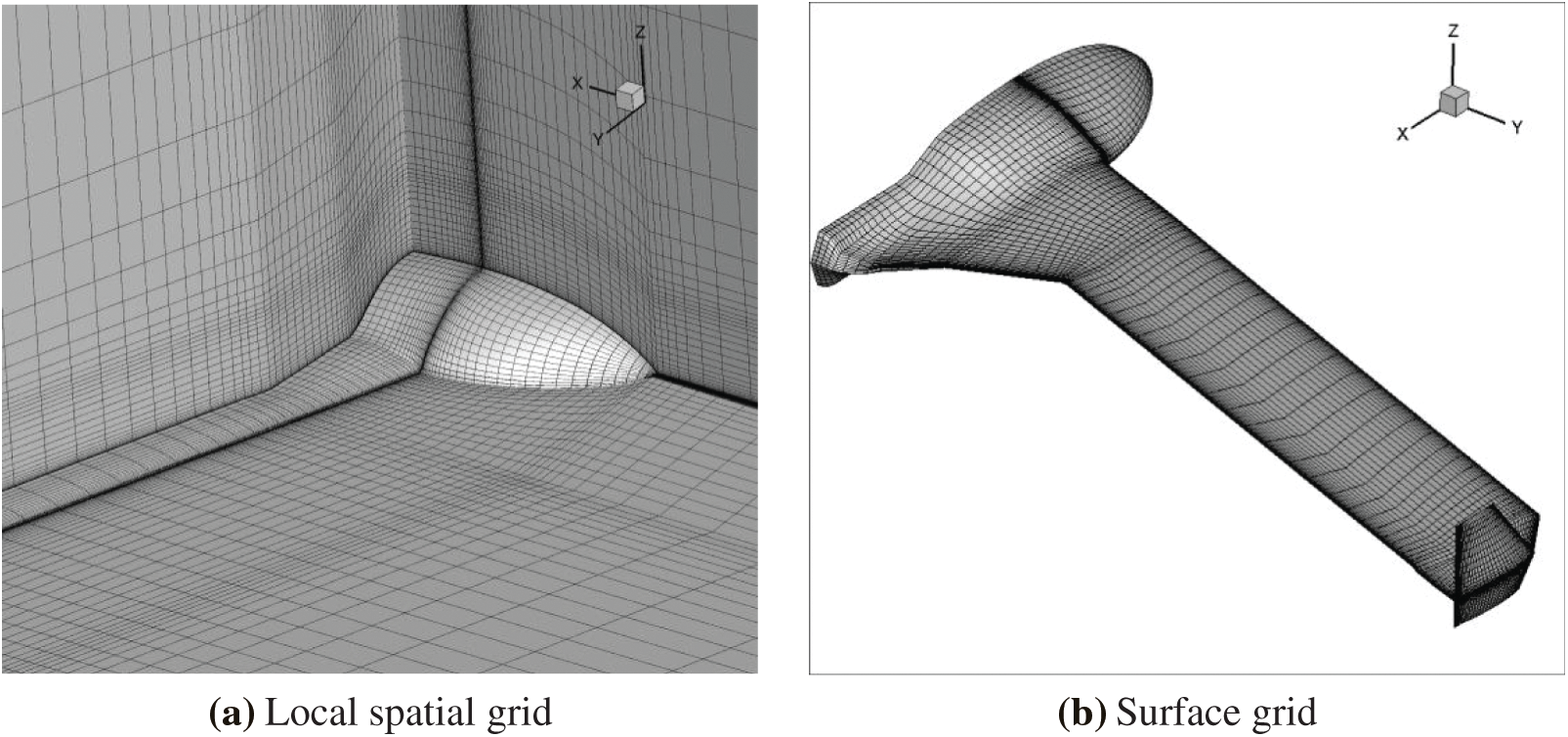
Figure 4: Local spatial grid and surface grid of flying wing model

3.2 Static Aeroelastic Trim

Only the longitudinal equilibrium of the vehicle is considered, and the thrust and drag are deemed to cancel each other. Two rigid body degrees of freedom in plunge and pitch are considered, which can be trimmed by adjusting the angle of attack (AoA) and the aileron deflection angle. The BFF speed of the flying wing vehicle is 41.6 m/s, calculated from Nastran software. Only elastic deformation is considered, the flight altitude is sea level, the Mach number is 0.122, and the coupled CFD/CSD time-domain calculations based on the N-S equation are used for the static aeroelastic trim calculations.

The static aeroelastic lift and pitch moments are calculated for three cases where the AoA and aileron deflection (upward is positive) are (0°, 0°), (0°, 1°) and (−1°, 0°), respectively. The calculation results are shown in Table 3. It is assumed that the AoA and aileron deflection angle satisfies a linear relationship with the lift and pitch moments in a small deformation range when elastic deformation is considered. From the calculation results, the aerodynamic derivatives Lα, Mα, Lδ and Mδ can be estimated. For example, Lα can be expressed as

Lα=∂L∂α=L(1∘,0∘)−L(0∘,0∘)Δα(21)

The aerodynamic derivative values are shown in Table 4.

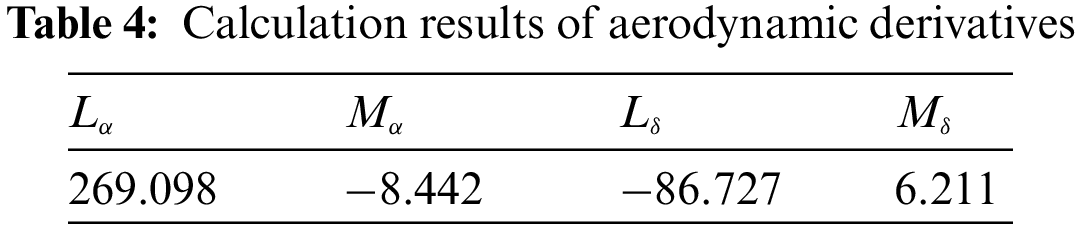
In this paper, the calculation is firstly carried out with (0°, 0°) points as reference points. In the trim state L(α,δ,qi)=81.5195N, My,CG(α,δ,qi)=0.

Table 5 shows the attitude and aerodynamic parameters of each trimmed calculation. The trim angle of attack and aileron deflection angle are chosen as (−0.62316°, 1.60930°). The convergence of the time response of the first four symmetric elastic modes (q(1)–q(4)) in the generalized coordinate under the trimmed condition is shown in Fig. 5.

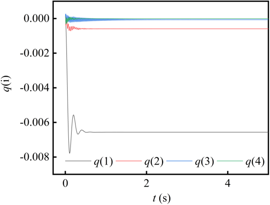
Figure 5: Time response of generalized coordinate of the elastic modes

3.3 Calculation of Body Freedom Flutter Boundary

Based on the static equilibrium state, the flight Mach number and altitude are not changed, the constant aerodynamic forces at this point are deducted, and the rigid body degrees of freedom in plunge and pitch are released for the BFF calculation. In CFD/CSD/6DOF time-domain calculations, an arithmetic mean vibration period is divided into 90 steps. The number of CFD virtual time iteration steps is used to reduce the residual value of each physical time step by two orders of magnitude or reach the maximum value of 200.

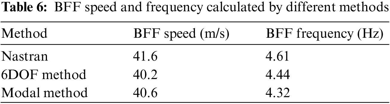
Figs. 6a, 6b show the time responses of rigid body displacements (plunge and pitch) and generalized coordinate of elastic mode calculated for the case of stiffness factor N = 1.0. It can be seen that the structural response diverges at Ma = 0.122 (41.6 m/s), indicating that the vehicle has fluttered. Fig. 5 shows the generalized coordinate time response of the elastic mode calculated without considering the sink and pitch, whose structural vibration converges. The comparison can be concluded that at this time the vehicle undergoes BFF with the participation of rigid body motion.

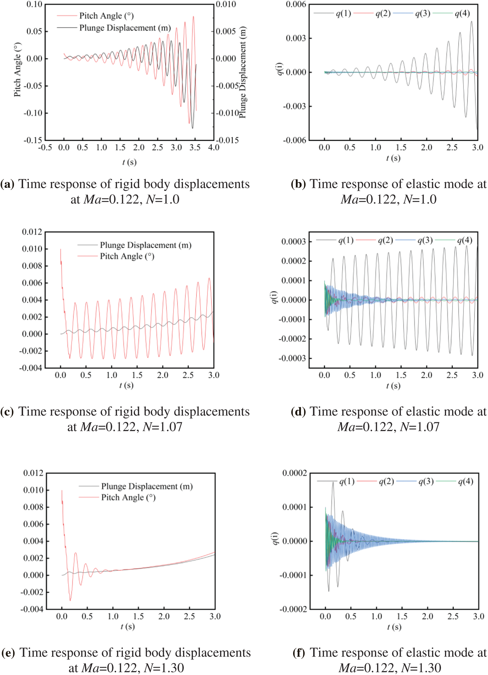
Figure 6: Time histories of rigid displacement and generalized coordinates of elastic mode at N = 1.0, 1.07, and 1.30 using BFF solver

Further, the variable stiffness method is used to increase the stiffness coefficient N and gradually approach the critical flutter state. By calculation, the stiffness factor in the critical state is N = 1.07. The time response at this time is shown in Figs. 6c, 6d. Continuing to increase the stiffness factor to 1.30, the calculated time response converges as shown in Figs. 6e, 6f. Through the variable stiffness technique, it can be seen that the flutter speed of the flying wing vehicle is 40.2 m/s and the flutter frequency is 4.44 Hz.

Rigid body motion is simulated by rigid body mode to analyze the BFF characteristics. The stiffness factor in the critical state is N = 1.05, and the general coordinate response is shown in Fig. 7. The variable stiffness technology can be used to calculate the flutter speed of the flying wing vehicle which is 40.7 m/s and the flutter frequency is 4.32 Hz.

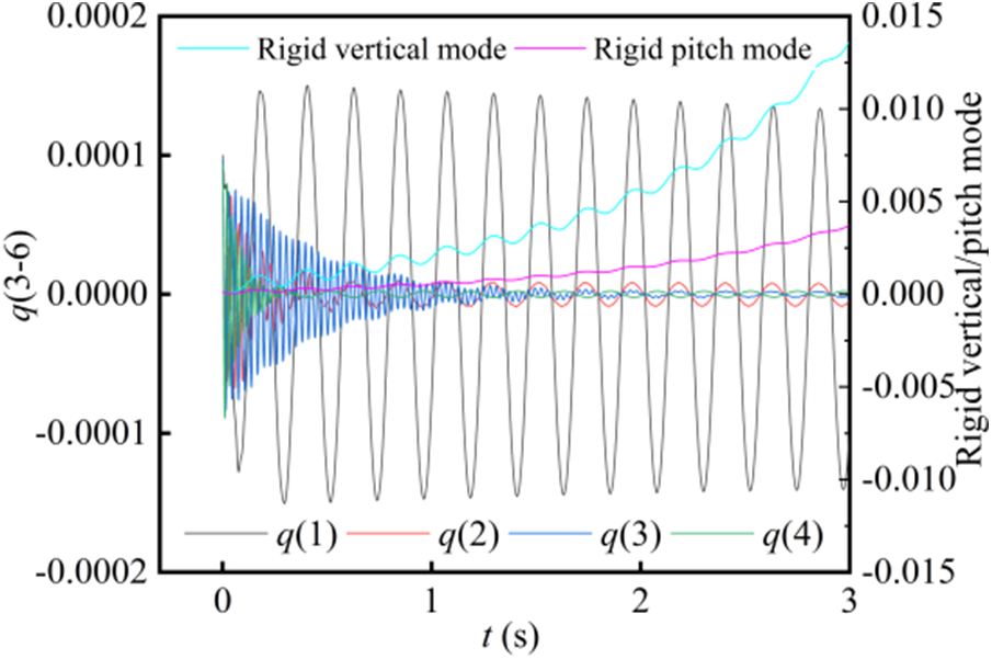
Figure 7: Time histories of generalized coordinates of the rigid and elastic mode of flying wing model at N = 1.05 using BFF solver

The corresponding results from Nastran are 41.6 m/s and 4.61 Hz. Table 6 summarizes the flutter speed and frequency calculated by the 6DOF method, modal method, and Nastran software. The calculation results of different methods are consistent, which proves the reliability of the CFD/CSD/6DOF time-domain BFF prediction method.

4  BFF Characteristics Influence Factors

In this section, the BFF characteristics influence factors are investigated using the BFF calculation method developed in the previous section. One of the objectives of this study is to explore the method of passively increasing the BFF speed. Body freedom flutter mainly involves short-period modes and 1st bending modes, while the frequencies of short-period and 1st bending modes can be changed by changing structural parameters. To consider the computational efficiency, this section adopts the Euler/CSD/6DOF numerical simulation method to study the effects of plunge motion, the center of mass position, and pitch inertia on the BFF.

Fig. 8 shows the time responses of rigid body displacements and the generalized coordinate of elastic mode in the BFF critical state calculated by the Euler/CSD/6DOF method. The critical state stiffness coefficient is N = 1.20. The flutter speed is 38.0 m/s, and the flutter frequency is 3.97 Hz. Ignoring viscosity, the unsteady aerodynamic force increases, making the flutter velocity calculated by the Euler equations smaller than that by the N-S equations.

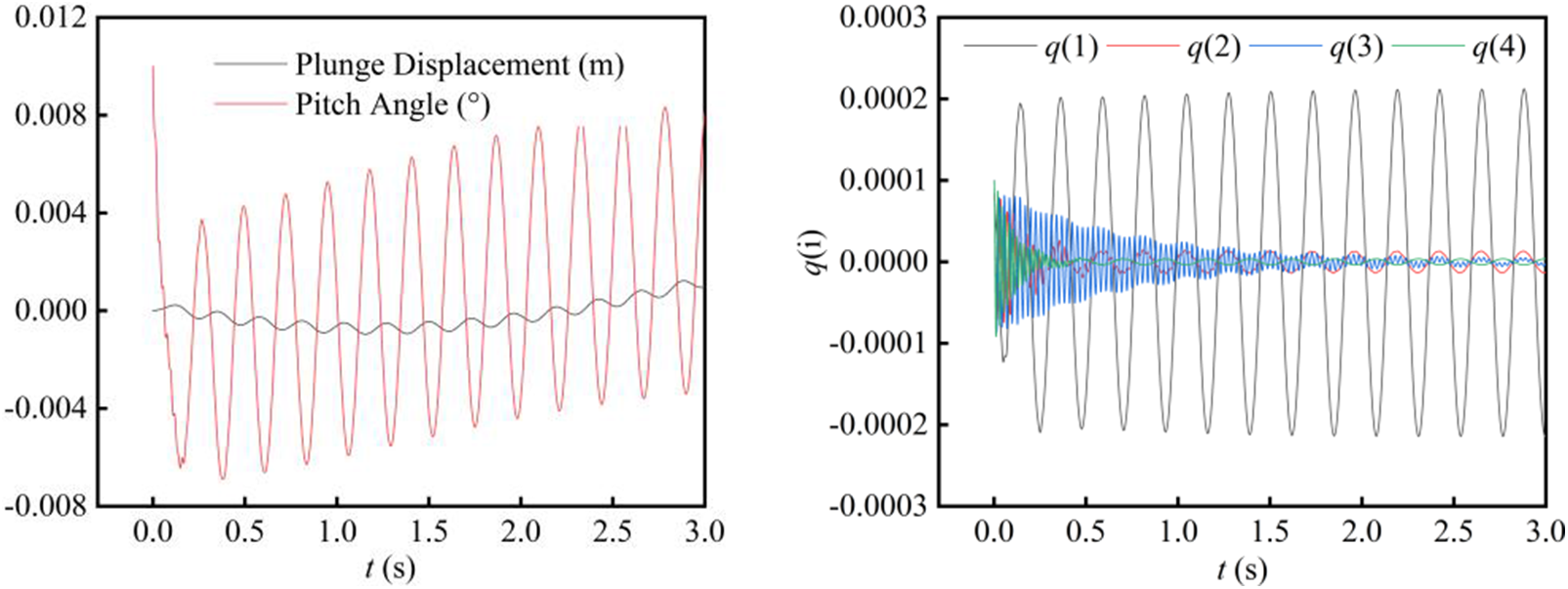
Figure 8: Time histories of rigid displacement and generalized coordinates of elastic mode in BFF critical state at N = 1.20 using Euler equations

4.1 Effect of Plunge Motion on the BFF Characteristics

Constrain the plunge degrees of freedom of the vehicle, and carry out the BFF calculation under the same static equilibrium shape and flight state to explore the influence of plunge motion on the BFF. Fig. 9 shows the time response of rigid body displacement and elastic mode in the critical state of BFF under the constraint of plunge freedom. Its critical stiffness coefficient is N = 3.80. It can be calculated that the BFF speed is 21.34 m/s, and the BFF frequency is 1.51 Hz. The BFF speed and frequency are lower than the case of considering the plunge motion.

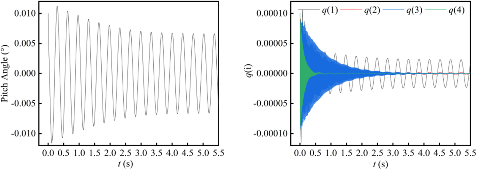
Figure 9: Time response of rigid body displacement and elastic mode in the BFF critical state under the constraint of plunge freedom

To explore the mechanism of the influence of the plunge on the BFF characteristics, the longitudinal stability characteristics of the vehicle when releasing or constraining the plunge degrees of freedom are calculated by coupling CFD/6DOF in the time domain. Fig. 10 compares the time response of the pitch angle of the two cases. It can be concluded that the aerodynamic damping of the vehicle is large when considering the plunge motion compared with the constrained plunge degrees of freedom. So the vehicle can recover to stability faster. However, in the case of constraints, the attenuation speed of the short-period mode is slow, so the BFF is more likely to occur. This is a good explanation for the phenomenon that the BFF speed of constraining the plunge degrees of freedom is lower than releasing the plunge degrees of freedom.

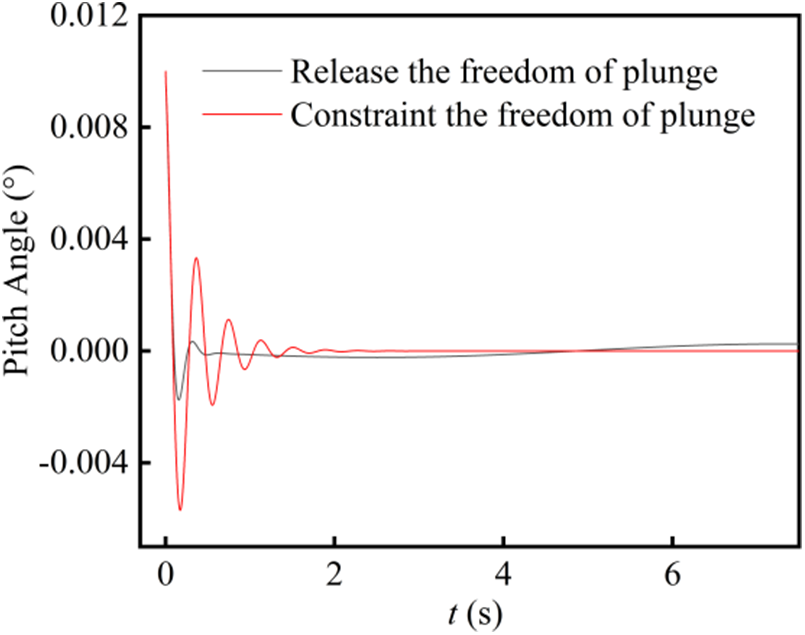
Figure 10: Time response of the pitch angle of two cases calculated by time-domain CFD/6DOF method

4.2 Effect of the Center of Mass Position on the BFF Characteristics

The finite element model of the flying wing vehicle is modified by shifting the mass block on its fuselage forward to change the center of mass. The flutter characteristics are calculated for four cases of 2 cm, 4 cm to 8 cm forward shift of the center of mass by the BFF solver.

The stiffness coefficients, flutter velocity, and flutter frequency for each critical state are given in Table 7. Fig. 11 shows the trend of flutter velocity and flutter frequency with the position of the center of mass. As the center of mass position gradually moves forward, the flutter speed and frequency increase. The reason mainly includes two factors: on one hand, the pitch inertia increases due to the forward movement of the center of mass, so the flutter speed increases; on the other hand, because the center of mass moves forward, the vehicle static stability margin increases, and the short-period modal damping increases, resulting in the more stable vehicle, so the flutter speed increases. Because the short-period modal frequency increases with the speed, the flutter frequency increases.

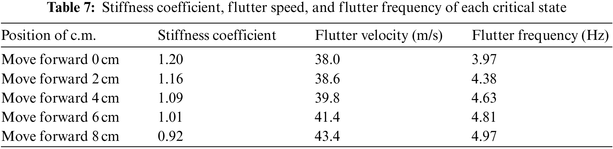
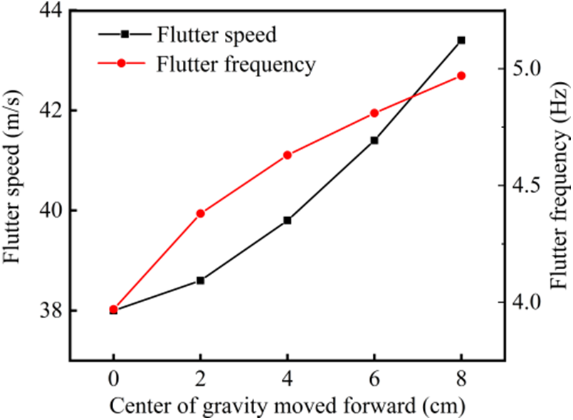
Figure 11: Influence law of center of mass position on BFF characteristics

4.3 Effect of Pitch Inertia Position on the BFF Characteristics

By changing the pitch inertia of the vehicle, the BFF characteristics are calculated for five cases of pitch inertia reduce by 20%, increased by 20%, and 40% up to 80%.

Table 8 gives the stiffness coefficients, flutter speed, and flutter frequency corresponding to the critical state of the flutter at each rotational inertia. Fig. 12 shows the trend of flutter speed and flutter frequency with the rotational inertia. As the rotational inertia gradually increases, the flutter speed increases while the frequency decreases. The main reason is that the short-period mode frequency decreases with the increase of rotational inertia, which makes the interval between the first-order bending mode and the first-order bending mode larger and makes it more difficult to occur the BFF, so the flutter speed increase.

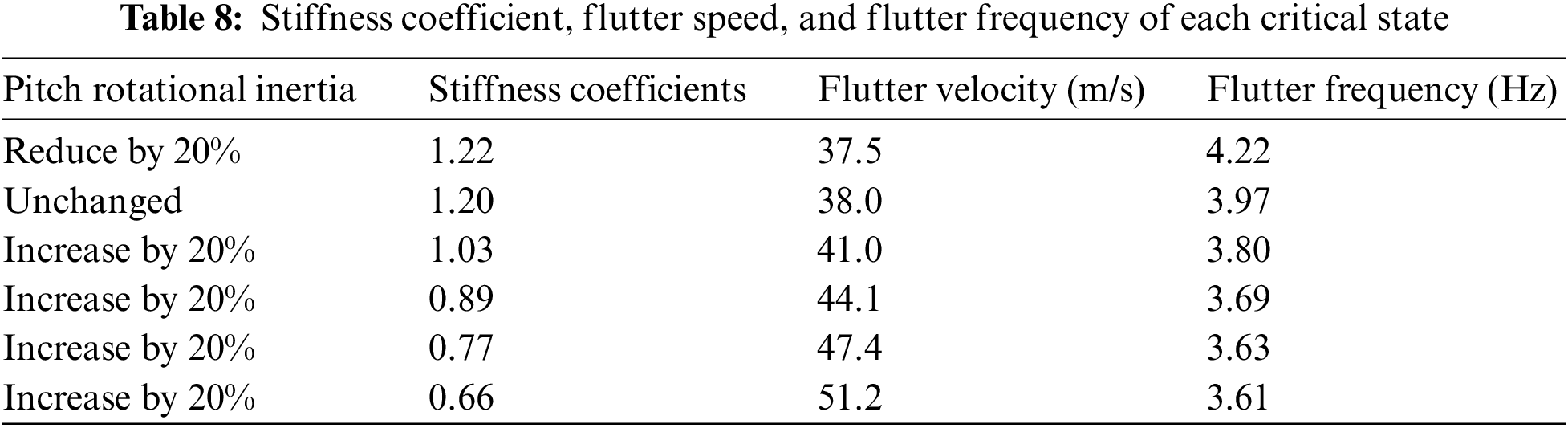
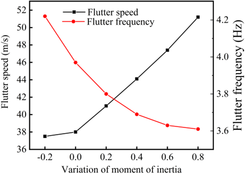
Figure 12: Influence of pitch inertia on BFF characteristics

5  Conclusions

To simulate the vehicle attitude changes more accurately and intuitively in the BFF calculation, in this paper, the 6DOF equation is used to describe the rigid body motion instead of the rigid mode. A method for predicting the BFF based on CFD/CSD/6DOF is established. BFF calculation is carried out on a flying-wing aircraft model. Finally, the influences of plunge motion, position of the center of mass, and moment of inertia on the BFF characteristics of flying wing vehicles are briefly analyzed. From numerical analysis, we conclude as follows:

(1)   Current methods can accurately predict the BFF characteristics of the vehicle. The calculated flutter speed and the frequency are in agreement with the results from the Nastran software and the modal method.

(2)   The BFF speed of the flying wing vehicle can be improved by releasing the plunge constraints, moving the center of mass forward, and increasing the pitch inertia.

(3)   The current method can be extended to other aeroelastic behavior predictions involving rigid body motion.

Acknowledgement: This work was supported by the National Natural Science Foundation of China (Nos. 12102187, 11872212) and a project funded by the Priority Academic Program Development of Jiangsu Higher Education Institutions.

Funding Statement: This work was supported by the National Natural Science Foundation of China (No. 11872212) and a project funded by the Priority Academic Program Development of Jiangsu Higher Education Institutions.

Author Contributions: The authors confirm contribution to the paper as follows: study conception and design: Zhehan Ji, Tongqing Guo; data collection: Zhehan Ji, Tongqing Guo, Di Zhou, Binbin Lyu; analysis and interpretation of results: Zhehan Ji, Tongqing Guo; draft manuscript preparation: Zhehan Ji, Di Zhou; supervision: Zhiliang Lu. All authors reviewed the results and approved the final version of the manuscript.

Availability of Data and Materials: The data that support the findings of this study are available from the corresponding author upon reasonable request.

Conflicts of Interest: The authors declare that they have no conflicts of interest to report regarding the present study.

References

1. Wakayama, S., Kroo, I. (1998). The challenge and promise of blended-wing-body optimization. 7th AIAA/USAF/NASA/ISSMO Symposium on Multidisciplinary Analysis and Optimization, pp. 239–250.St. Louis, USA. [Google Scholar]

2. Wakayama, S. (2000). Blended-wing-body optimization problem setup. 8th Symposium on Multidisciplinary Analysis and Optimization, pp. 1–11. Long Beach, USA. [Google Scholar]

3. Huang, R., Hu, H. Y. (2021). Nonlinear aeroservoelasticity of aircraft. Advances in Mechanics, 51(3), 428–466. [Google Scholar]

4. Love, M., Zink, P., Wieselmann, P., Youngren, H. (2005). Body freedom flutter of high aspect ratio flying wings. 46th AIAA/ASME/ASCE/AHS/ASC Structures, Structural Dynamics and Materials Conference, pp. 1–23. Austin, USA. [Google Scholar]

5. Schweiger, J., Sensburg, O., Berns, H. J. (1985). Aeroelastic problems and structural design of a tailless CFC-sailplane. Proceedings of the 2nd International Forum on Aeroelasticity and Structural Dynamics, pp. 457–467. Aachen, Germany. [Google Scholar]

6. Nicolai, L., Hunten, K., Zink, P. S., Flick, P. (2010). System benefits of active flutter suppression for a sensorcraft-type vehicle. 13th AIAA/ISSMO Multidisciplinary Analysis Optimization Conference, Fort Worth, USA. [Google Scholar]

7. Burnett, E., Atkinson, C., Beranek, J., Sibbitt, B., Holm-Hansen, B. et al. (2010). Ndof simulation model for flight control development with flight test correlation. AIAA Modeling and Simulation Technologies Conference, Toronto, Canada. [Google Scholar]

8. Beranek, J., Nicolai, L., Buonanno, M., Burnett, E., Atkinson, C. et al. (2010). Conceptual design of a multi-utility aeroelastic demonstrator. 13th AIAA/ISSMO Multidisciplinary Analysis Optimization Conference, Fort Worth, USA. [Google Scholar]

9. Richards, P. W., Yao, Y., Herd, R. A., Hodges, D. H., Mardanpour, P. (2016). Effect of inertial and constitutive properties on body-freedom flutter for flying wings. Journal of Aircraft, 53(3), 756–767. [Google Scholar]

10. Guo, S., Jing, Z. W., Li, H., Lei, W. T., He, Y. Y. (2017). Gust response and body freedom flutter of a flying-wing aircraft with a passive gust alleviation device. Aerospace Science and Technology, 70(1), 277–285. [Google Scholar]

11. Huang, C., Wu, Z., Yang, C., Dai, Y. (2017). Flutter boundary prediction for a flying-wing model exhibiting body freedom flutter. 58th AIAA/ASCE/AHS/ASC Structures, Structural Dynamics, and Materials Conference, Grapevine, USA. [Google Scholar]

12. Lei, P., Guo, H., Lyu, B., Chen, D., Yu, L. (2021). Verification of a body freedom flutter numerical simulation method based on main influence parameters. Machines, 9(10), 243–257. [Google Scholar]

13. Theis, J., Pfifer, H., Seiler, P. J. (2016). Robust control design for active flutter suppression. AIAA Atmospheric Flight Mechanics Conference, San Diego, USA. [Google Scholar]

14. Danowsky, B. P., Lieu, T., Coderre-Chabot, A. (2016). Control oriented aeroservoelastic modeling of a small flexible aircraft using computational fluid dynamics and computational structural dynamics-invited. AIAA Atmospheric Flight Mechanics Conference, San Diego, USA. [Google Scholar]

15. Schmidt, D. K., Zhao, W., Kapania, R. K. (2016). Flight-dynamics and flutter modeling and analyses of a flexible flying-wing drone-invited. AIAA Atmospheric Flight Mechanics Conference, San Diego, USA. [Google Scholar]

16. Gaitonde, A. (1995). A dual-time method for the solution of the 2D unsteady Navier-stokes equations on structured moving meshes. 13th Applied Aerodynamics Conference, pp. 926–936. San Diego, USA. [Google Scholar]

17. Jameson, A., Schmidt, W., Turkel, E. (1981). Numerical solution of the Euler equations by finite volume methods using runge kutta time stepping schemes. 14th Fluid and Plasma Dynamics Conference, pp. 1259–1272. Palo Alto, USA. [Google Scholar]

18. Spalart, P., Allmaras, S. (1992). A one-equation turbulence model for aerodynamic flows. 30th Aerospace Sciences Meeting and Exhibit, pp. 1–22. Reno, USA. [Google Scholar]

19. Guo, T., Lu, Z., Wu, Y. (2009). A time-domain method for transonic flutter analysis with multidirectional coupled vibrations. Modern Physics Letters B, 23(3), 453–456. [Google Scholar]

20. Guo, T., Lu, Z., Tang, D., Wang, T., Dong, L. (2013). A CFD/CSD model for aeroelastic calculations of large-scale wind turbines. Science China Technological Sciences, 56(1), 205–211. [Google Scholar]

21. Guo, T., Zhou, D., Lu, Z. (2017). A double-passage shape correction method for predictions of unsteady flow and aeroelasticity in turbomachinery. Advances in Applied Mathematics and Mechanics, 9(4), 839–860. [Google Scholar]

22. Guo, T., Shen, E., Lu, Z., Ding, L. (2018). Structural deformation-based computational method for static aeroelasticity of high-aspect-ratio wing model in pressurized wind tunnel. Advances in Applied Mathematics and Mechanics, 10(5), 1158–1172. [Google Scholar]

23. Zhang, W., Jiang, Y., Ye, Z. (2007). Two better loosely coupled solution algorithms of CFD based aeroelastic simulation. Engineering Applications of Computational Fluid Mechanics, 1(4), 253–262. [Google Scholar]

24. Romanelli, G., Castellani, M., Mantegazza, P., Ricci, S. (2012). Coupled CSD/CFD non-linear aeroelastic trim of free-flying flexible aircraft. 53rd AIAA/ASME/ASCE/AHS/ASC Structures, Structural Dynamics and Materials Conference, Honolulu, USA. [Google Scholar]

25. Lu, Z. L., Guo, T. Q., Guan, D., (2004). A study of calculation method for transonic flutter. Acta Aeronautica et Astronautica Sinica, 4, 214–217. [Google Scholar]

26. Burnett, E. L., Beranek, J. A., Holm-Hansen, B. T., Atkinson, C. J., Flick, P. M. (2016). Design and flight test of active flutter suppression on the X-56A multi-utility technology test-bed aircraft. The Aeronautical Journal, 120(1228), 893–909. [Google Scholar]

27. Li, W. W., Pak, C. G. (2014). Aeroelastic optimization study based on the X-56A model. AIAA Atmospheric Flight Mechanics Conference, Atlanta, USA. [Google Scholar]