Learning Discriminatory Information for Object Detection on Urine Sediment Image

1  Introduction

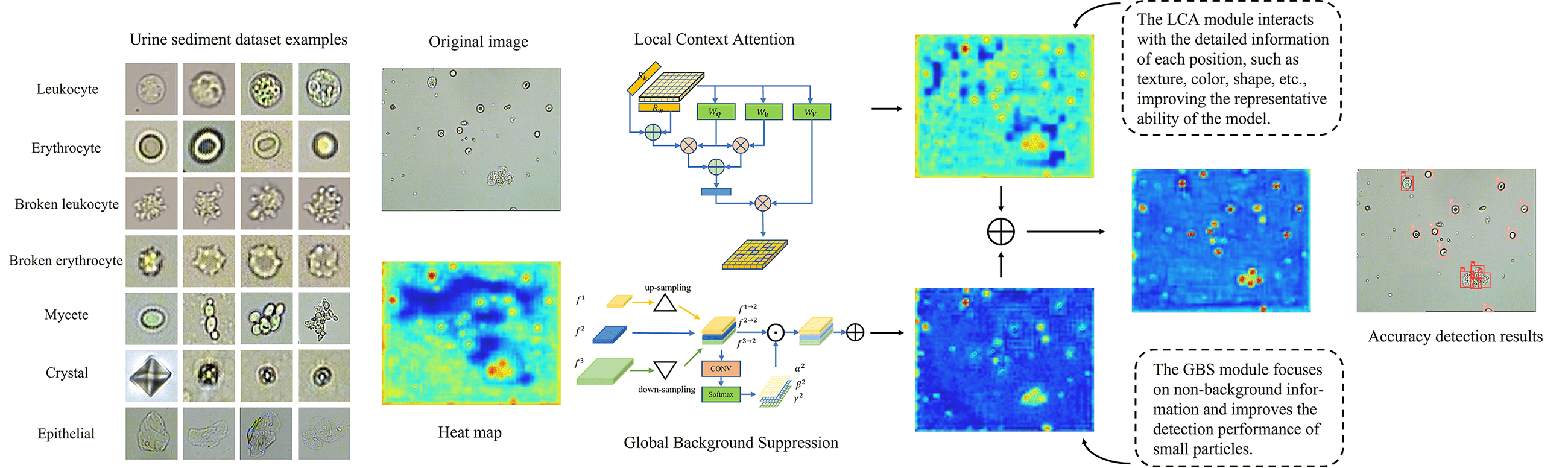
In clinical practice, there are typically two primary methods used to test urine specimens. These include the urine routine test and the urine sediment examination. Urine routine test indicators generally include urine red blood cells (RBCs), white blood cells (WBCs), and urine protein. Based on the indicators of urine routine tests, it is possible to determine whether a patient has the renal tubular disease, blood disease, glomerular function, liver and gallbladder disease, etc. [1]. For example, a large number of RBCs, calcium oxalate crystals (CAOXs), and hyaline casts (HYALs) indicate the presence of urinary tract calculi [2]. However, the accuracy of urine routine tests can be easily affected by the patient’s metabolic problems and drug use. Consequently, medical professionals are increasingly turning to urine sediment examination for certain important diagnoses. Urine sediment examination is one of the most important methods, providing a scientific basis for clinical diagnosis and improving the accuracy of diagnoses [3]. Manual testing is time-consuming, labor-intensive, and subjective, which requires highly trained technicians. By detecting the amount of various urine sediment in sampling images, the amount of urine sediment in a sample can be calculated. Markedly elevated levels of red blood cells in urine can be indicative of the presence of kidney disease, lower urinary tract disease, and extrarenal disease. Similarly, a substantial increase in white blood cells may suggest the possibility of inflammation within the urinary system, while increased epithelial cells may indicate the presence of inflammation. The presence of an increased amount of crystals in urine may signal the presence of urinary stones, and high levels of mycetes are typically observed in patients with diabetes. Therefore, analyzing the urinary sediment content from a urine sample is a valuable and informative method for evaluating the condition of various organs within the urinary system.

Object detection has made great progress in the field of natural images, remote sensing images and medical images [4,5]. In the urine sediment examination, object detection automatically and efficiently locates and classifies particle instances from microscope images, which is precisely the task of object detection. To detect the images taken by the urine sediment analyzer, combining online and offline integration with the Internet is a trend that has emerged in recent years [6]. We deploy the model on the server and then can get the amount of various urine sediment by uploading the urine sediment images to the server for detection, which certainly helps medical personnel save time and effort. This application requires fast speed to meet real-time detection needs. Although the machine learning method [7] is effective in stabilizing features and handling high-dimensional and low-dimensional data, its detection speed can sometimes be slower than desired. Like Support Vector Machine (SVM) uses Histogram of Oriented Gradient [8] to extract features, which takes about 1 s, and its detection performance is limited by intra-class differences.

The deep learning method is significant because of its high speed and accuracy in urine sediment detection. CNN-based (Convolutional Neural Network) algorithms combine with traditional feature processing methods are not efficient. Ji et al. [9] added branches to identify and classify small objects separately, such as erythrocytes and leukocytes. The branches classify particles based on edge features in the segmented region. However, it is not easily generalizable to other categories, as each branch needs to be trained independently for a specific category. The CNN-based algorithms combined with the graphical neural network [10] can establish the relationship between features to improve classification accuracy. At present, convolution neural networks are getting deeper and deeper, and GCN is difficult to adapt. One-stage target detection algorithms like YOLOs [11,12] predict directly on the feature maps and take less time during inference. Introducing the attention mechanism into the deep learning model has proven to be an effective approach for enhancing the detection performance of small urine sediments [13]. This method only utilizes the spatial information of the current layer’s feature map, without interacting with the feature maps of other layers.

Datasets are the foundation of the computer vision on which the proposed methods are evaluated. Many natural image datasets have been proposed in recent years, facilitating the development of deep learning algorithms. In medical images, a few urine sediment datasets are publicly available, and only a few contain comprehensive annotation and classification. This manuscript annotates a urine sediment dataset to facilitate the application of deep learning in medical images. The challenge for the urine sediment dataset is that most particles are small-scale in the dataset. What’s more, there are locally dense cases in urine images which means particles overlap each other. Dense object detection is also a big challenge for detectors. Generic object detection algorithms contain [14] a large number of parameters, which tend to overfit the algorithm if trained on a dataset with a small number of samples, and these algorithms have poor detection performance for small objects.

Based on the above observations, we propose the lightweight detector discriminatory-YOLOv5s based on [12], which takes advantage of high speed and outstanding detection performance. YOLOv5 is convenient for adjusting the model size by changing hyperparameters. What’s more, it is easy to be deployed to the chip due to the reproducibility of the structure. This detector achieves better performance than normal object detectors with the proposed local context attention (LCA) module and global background suppression (GBS) module. These two modules improve the models’ discriminatory ability. The LCA module makes the model pay more attention to context information around the particles to distinguish dense particles. The GBS module is designed to reduce the impact of background by fusing different level features. The feature fusion highlights the low-level features for better classification and localization. Our contributions are as follows:

•   We present a new urine sediment dataset called UriSed2K containing 2465 images with 7 categories. This dataset contains 29450 annotated labels.

•   We design a novel intelligent automatic system, which contains a detector called discriminatory-YOLOv5s with LCA module and GBS module for object detection on urine sediment images. The LCA module is designed to distinguish dense particles. This module helps the model find correlated features around the particles by capturing context information. The GBS module is proposed to suppress background information by learning the importance weight of feature maps. It makes the model focus on non-background information and improves the detection performance of small particles.

•   Our proposed method achieves better performance than the mainstream object detection methods in two urine sediment datasets, while our model includes fewer parameters.

The following content of this manuscript is summarized as follows. We briefly review the research related to our work in Section 2. We describe in detail the specifics of our annotated dataset in Section 3. Then, the specifics of LCA module and GBS module are given in Section 4. The experimental results are presented in Section 5. Finally, Section 6 summarizes our results and provides some ideas for future work.

2  Related Work

2.1 Urine Sediment Image Dataset

In recent years, the size of image datasets has shown an increasing trend, from VOC [15] to ImageNet [16], MS-COCO [17]. The Pascal VOC dataset contains 21,500 images in 20 classes. The MS-COCO dataset contains over 300,000 images in 80 classes, 200,000 annotated, and more than 2 million instances in the entire dataset. The ImageNet dataset has more than 14 million images across more than 20,000 categories. More than 1 million of these images have clear category annotations and bounding boxes for the location of objects in the image.

Compared to the vast natural image datasets, medical image datasets are relatively small in scale [18]. We found a few existing works on urine sediment datasets for recognition or detection: the dataset in [19] contains 1671 images, which is used for recognition by using deep learning. The urine sediment dataset USE [20–22] contains 5376 useful urinary microscopical images after filtering, resulting in 43000 meaningful instances. Undoubtedly, it takes a lot of time to remove images that only include noise. The research [9] collects 650 images for 10 categories and gets 300000 segments from these images. UMID (Urine Microscopic Image Dataset) [23] comprises 367 annotated microscopic images of urine sediment of dimensions (1280,720). The UMID contains 3 types of cells, RBCs, WBCs and epithelial cells. What’s more, annotating labels requires relevant medical expertise. Since urine sediment images are difficult to obtain and labeling them is labor intensive, urine sediment datasets are valuable, and most are not publicly available.

2.2 Object Detection of Urine Sediment Images

There are many proven network models in the field of object detection. Object detection models are similar in extracting features. These features are extracted bottom-up from the image by convolution. Two-stage models such as Faster R-CNN [14] select regions that may contain objects, so they need to generate a large number of proposals which takes more time to process. Two-stage models take advantage of high precision. One-stage models such as YOLOs [11,12], FCOS [24], make predictions directly for each region of the image without the process of generating proposals. Their inference speeds are fast at the expense of precision, but the expense of precision is tolerable in practical application scenarios.

These network models are originally designed for natural image datasets such as VOC, COCO, which have complex backgrounds and different categories. These models contain many parameters, and the models require sufficient data for adequate training. Urine sediment datasets are usually small in size, and these models may be overfitted when trained directly on these datasets. In practice, lightweight models containing fewer parameters should be used, which are also easy to implement. The distinctive characteristic of the urine sediment dataset is the small objects. Most of the particles take up less than 1% area of the image. In the field of medical images, feature fusion can use its own feature information to improve detection performance significantly [25]. The Feature Pyramid Network (FPN) [26] fuses feature maps of various scales from top to bottom, transmitting semantic information from deep feature maps to shallow ones, which improves the detection performance of small objects. The FPN combined with DenseNet [22], alleviates the problem of category confusion in the urine sediment images and performs well in an image with dozens of small particles. B-PesNet enriches semantic information in shallow layers so that the deep convolution layers can leverage more information when concatenating feature maps [27]. Reference [21] exchanged context information between multi-scale features in the FPN and then fuse these features by element-wise addition. The Path Aggregation Network (PAN) [28] followed behind FPN and transmits low-level information from the bottom up to the high level.

CNNs are able to capture local features due to the nature of convolution. However, CNNs are limited by the receptive field and are less capable of modeling regions outside the receptive field. In order to interact between feature map pixels, it is becoming increasingly common to use self-attention architecture for CNN models to obtain global modeling capabilities [29].

3  UriSed2K Dataset

We collect 2465 unstained images that are captured by an automatic urine sediment detector. The automatic urine sediment detector can automatically detect the position of the sample, aspirate it, mix it, and allow it to settle. It then captures an image of the sample through a microscope in the catheter. The resolution of the urine sediment microscopy images is 800 by 600 pixels. Fig. 1 displays the seven major categories present in our urine sediment dataset, which include leukocyte, erythrocyte, broken leukocyte, broken erythrocyte, mycete, crystal, and epithelial cell.

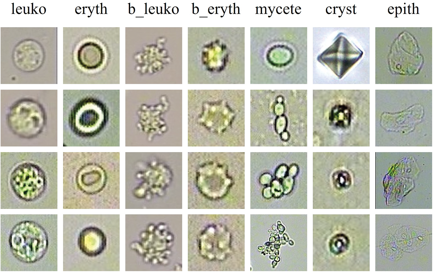
Figure 1: The samples of seven categories of particles in the UriSed2K

We annotate the images using rectangular boxes with labels in the VOC format. Each box includes the category value and the coordinates of the upper left and lower right corners, which are c, x1, y1, x2, y2. To enable a wider range of algorithms to be trained on this dataset, we have developed scripts to convert the dataset from the VOC format to either YOLO or COCO format. The YOLO format annotations include the center coordinates of the bounding box and its width and height relative to the original image. The COCO format annotations are similar to VOC format and are saved in a single JSON file for all images. According to the labels we annotated, we draw two figures: Fig. 2 shows the number of seven particles in our dataset, Fig. 3 shows the distribution of rectangular boxes’ ratio of width and height. There are three main challenges in the urine sediment dataset:

Small-scale object: Fig. 3 shows the distribution of rectangular anchor boxes’ size. In our dataset, the area of the largest object is no more than 14% of the whole image. Over 80% of the particles take up less than 1% area of the image. About 50% of the particles are smaller than 0.5% of the image area. This strongly suggests that the urine sediment dataset can be regarded as a small-scale object detection dataset.

Intra-class variation: Fig. 1 shows the various shapes of the same particles. The shapes of mycete are determined by its reproduction. The shapes of crystals depend on the formation conditions. Additionally, the appearance of particles can be affected by various shooting conditions, including the intensity of the light source and the magnification level.

Locally dense distribution: The distribution of particles in the urine images is globally sparse. Notably, even after dilution, some particles continue to cluster together. It is challenging to detect these aggregated particles one by one.

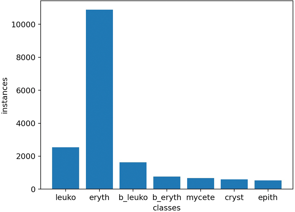
Figure 2: The number of particles. The numbers of various particles from left to right are 4322, 18335, 2723, 1148, 1083, 894, and 945, respectively. The letter ‘b’ stands for ‘broken’

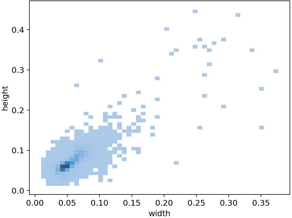
Figure 3: The distribution of rectangular anchor boxes’ size. The value on the coordinate axis indicates the ratio of the width and height of the anchor box to the width and height of the image. The darker the color of the pixel point, the more anchor boxes are on that scale

4  Methods

In view of the characteristics of the urine sediment dataset, we propose two modules to improve the detection performance in detecting small objects by stronger discrimination. Fig. 4 shows our network model with two modules.

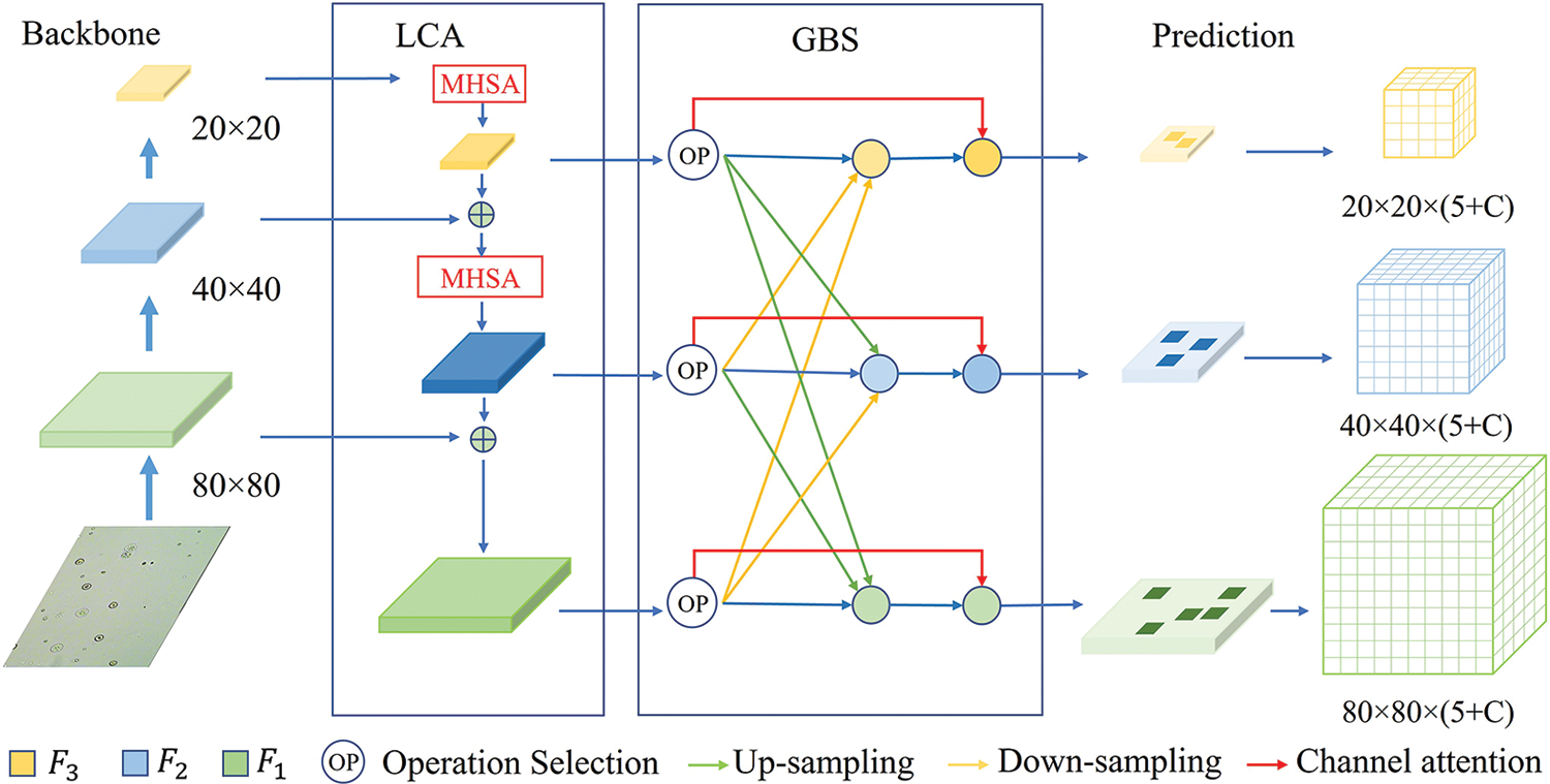
Figure 4: The network of the discriminatory-YOLOv5s. The backbone extracts feature maps at different levels. The local context attention (LCA) module captures long-range information and concatenates feature maps. The global background suppression (GBS) module suppresses the background through feature fusion. The prediction head is responsible for predicting three scale feature maps. The variable C represents the number of classes in the dataset. The value of 5+C contains information about the predicted bounding box, including the center coordinates, height, width, objectness score, and probabilities of C categories

4.1 Local Context Attention Module

Determined by the properties of convolutional neural networks, the low-level feature maps contain more detailed features, which are effective for the model in detecting and predicting small particles. However, in the urine sediment dataset, particles tend to aggregate and block each other, making it difficult for models relying solely on low-level features to locate and classify individual particles. To distinguish these aggregated particles, we introduce self-attention mechanism to make the model focus on regions outside the receptive field. We propose the Local Context Attention (LCA) module based on FPN [26] incorporating the self-attentive mechanism. The module transfers high-level semantic information after attention to low-level features. Inspired by [29] and [30], we design several multi-head self-attention (MHSA) layers with relative position encoding to the FPN, overcoming the limitation of the receptive field by the convolutional kernel size. The improved model can increase the interaction between information from distant locations in the feature map.

To capture the correlation between two positions in the feature map, the MHSA layer attends to the features at those positions and computes a weighted sum of them. We then concatenate the resulting high-level feature maps with low-level feature maps to increase the model’s attention on dense areas in the low-level feature maps. As shown in Fig. 4, we add the MHSA layers to different scale feature maps. To fit these feature maps, we design the length of the position encoding to adapt to the input feature map’s scale. Adjusting the length of the position encoding to the input feature map’s scale is necessary to ensure that the relative positions of features are accurately captured across all feature map scales. The position encoding is used to represent the spatial relationships between features in the input feature map, and its length needs to be adjusted according to the scale of the feature map to account for variations in the relative distances between features at different scales.

In the MHSA layer, the input feature map is divided into multiple heads equally to allow for better capturing of the spatial relationships between pixels. Specifically, we divide the feature map into four heads based on the channel dimension in our module. Fig. 5 shows the architecture of the MHSA layer with position encoding. For each head, we compute query, key, and value projections by 1×1 convolutions. These projections are used to compute attention scores between each pair of positions in the feature map. To account for the relative positions of features, we use two learnable vectors for each head. These position encodings are added to the query and key projections before the attention scores are computed. The context information content_context is computed by q, k.

content_context=qT⊗k(1)

where T represents transpose, and ⊗ is the matrix multiplication. The content_context contains correlation information between two pixels, which represents the importance of each location in the input feature map relative to q. In order to consider location information in space, we introduce relative position encoding to the feature maps.

r=(Rh⊕Rw)(2)

where r is the relative position distance encodings, Rh and Rw are the learnable vectors to represent the relative position distances along the height and width dimensions, respectively, and ⊕ is the element-wise sum. The position of each pixel point can be represented according to the offset in the height and width dimensions.

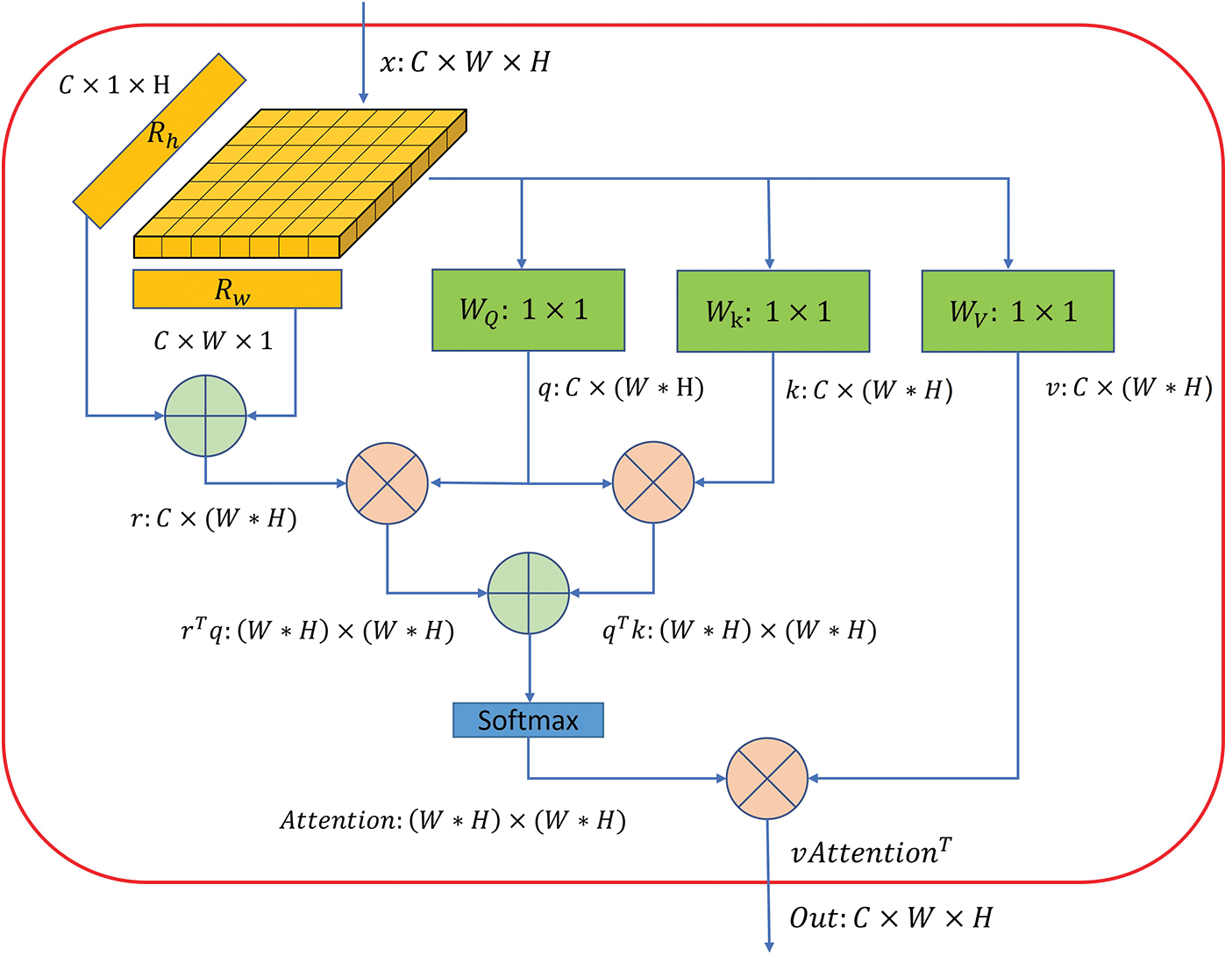
Figure 5: The architecture of one of the heads in a multi-head self-attention layer. C, H and W demonstrate the channel number, height and width of the given feature map. WQ, WK, and WV are three different 1×1 convolution layers, Rh and Rw are learnable vectors, and their lengths are initialized based on the input feature map, ⊕ is the element-wise sum, ⊗ is the matrix multiplication. The head focuses on the important positions of the given feature map, which is determined by the generated attention map

content_position=rT⊗q(3)

where content_position is the position information, it is obtained by matrix multiplication between the transposed position encoding rT and the query projection.

Attention=softmax(content_context⊕content_position)(4)

where Attention is the attention map which is the summary of content_context and content_position after softmax. The value in the attention map is ∈(0,1), which represents the relative importance of different positions in the input feature map.

SA(q,k,v,Rh,Rw)=v⊗AttentionT(5)

where v is the value projection. SA is the reweighted feature map that reflects the relation between two pixels of the feature map.

Headi=SA(qi,ki,vi,RhiRwi)(6)

where i∈[1,n], n is the preset number of head.

Out=Concat(Head1,Head2,…,Headn)(7)

where Out is concatenated by all heads, the parameters in each head are independent. After the above operations, we utilize MHSA to enhance the position of feature maps with high similarity in each feature map before fusion. The LCA module overcomes the limitation of the receptive field and interacts with the detailed information of each position, such as texture, color, shape, etc., improving the representative ability of the model.

4.2 Global Background Suppression Module

From Section 3, we learn that the distribution of particles in urine images is globally sparse, which means that the background takes up most of the image and provides little information. When we humans look at images, we actively ignore the background to focus on the objects we are interested in. To enable our model to do the same, we have designed the GBS module, which assigns low weights to the background and allows the model to ignore it. The GBS module is inspired by [31] and fuses different levels of features by learning the importance weights of spatial information adaptively. This means that low-level features such as edges, corners, colors, and shapes are given more importance for localization. After adding the GBS module, the model pays much less attention to the background, just as our human visual system does.

Fig. 6 shows the feature fusion of level 2 in the GBS module. For each level, the process of fusing the futures at the corresponding level l is as follows:

Fl=αijl⋅op(f)ij1→l+βijl⋅op(f)ij2→l+γijl⋅op(f)ij3→l(8)

where Fl refers to the target level feature, and l,n are both integers in the set {1,2,3}. fn→l represents the feature map that has been resized from level n to match the size of level l. αl, βl, γl represent the spatial importance weights of level l, which are shared across all channels. i and j denote the position of the feature map. The weights of each point are obtained by the softmax function, αijl+βijl+γijl=1 and αijl,βijl,γijl∈(0,1). For example, getting the weight of αl as follows:

αijl=eλfij1→leλfij1→l+eλfij2→l+eλfij3→l(9)

where λfijn→l are control parameters, which are obtained by convolution. The channel of resized feature maps is compressed by two 1×1 convolution layers.

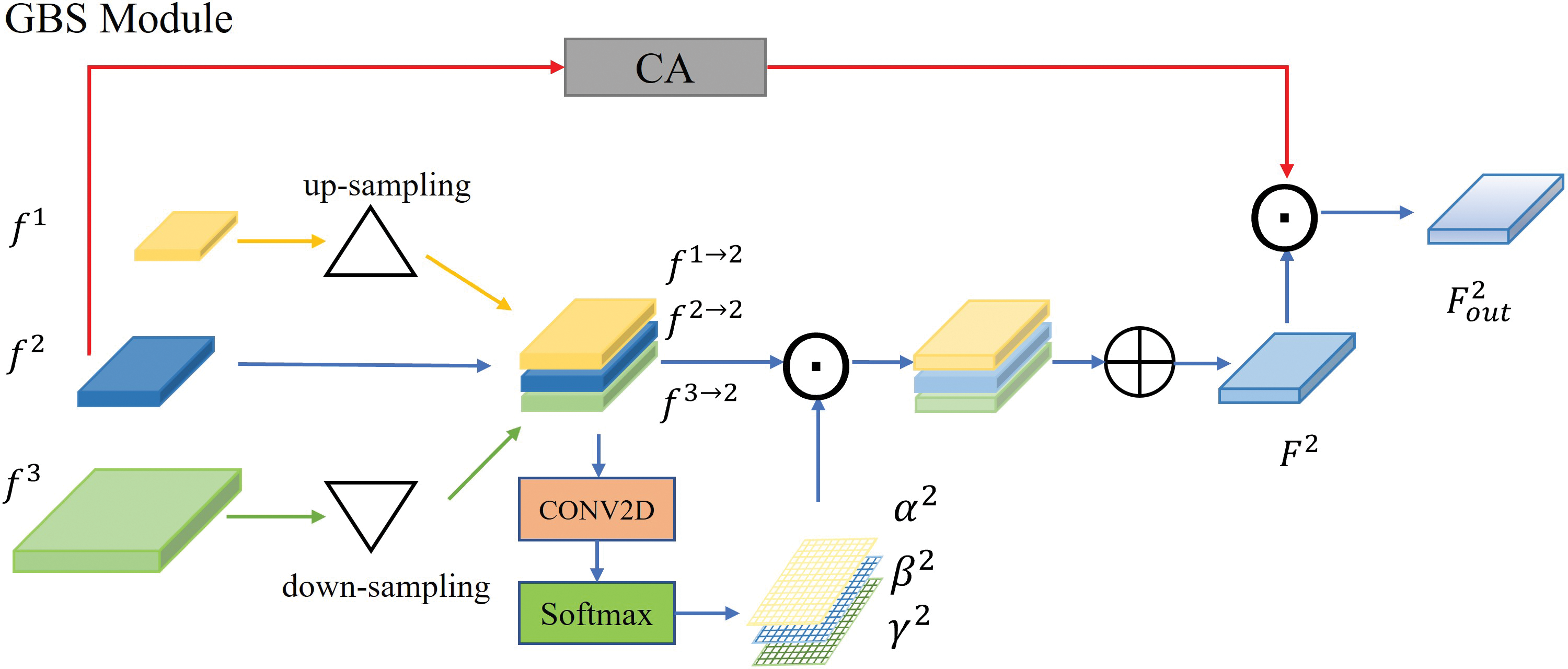
Figure 6: The details of level 2 in the GBS module. △, ▽, ⊙, ⊕ represent up-sampling, down-sampling, element-wise multiplication and element-wise sum, respectively. α, β, γ are the spatial importance weights. f1, f2, f3 are the feature maps. f1→2, f2→2, f3→3 are the feature maps after resizing. The CA is a channel attention mechanism

op={△|l−n|,if  Cn>Cl,▽|l−n|,if  Cn<Cl,None,otherwise.(10)

where op is the resizing operation, △ and ▽ represent the up-sampling and down-sampling, respectively. In the LCA module, the size of the feature map becomes larger and the number of channels decreases. Therefore, the resizing operation can be determined by the number of channels. For up-sampling, we use a 1×1 convolution layer to compress dimension to the same level l. Then the feature map is enlarged by nearest interpolation, where the multiplier for spatial size is equal to 2×|l−n|. For down-sampling, if |l−n|=1, we use a 3×3 convolution layer with stride 2, similar to the down-sampling in the YOLOv3 backbone. It is different when |l−n|=2, a 3×3 kernel size max pool layer with stride 2 added before the convolution layer.

αl, βl, γl are learned from the spatial information and are shared across each channel. From the perspective of channel importance, we add channel attention to enhance cross-channel interaction. Inspired by [32], we add simple channel attention to Fl. This channel attention first compresses the spatial information of each feature map using global average pooling and then learns the importance of each channel using one-dimensional convolution across channels, which can consider both local channel information and global channel information with low computational complexity. The last output is defined as follows:

Foutl=Fl⊙(CONV(GAP(fl)))(11)

where CONV represents the 1 dimensional convolution with kernel size 5, ⊙ represents the element-wise multiplication. GAP represents the global average pooling, and fl is the feature of level l before operation. The fusion parameters in this module are obtained through convolution and are able to participate in standard back-propagation for learning. Through training, these parameters can be effectively adjusted to reweight the feature maps and reduce the weight of background regions, leading to an improvement in the model’s detection performance.

4.3 Loss Function

Same as normal object detection algorithms, the loss consists of three components:

Lall=λclsLcls+λboxLbox+λobjLobj(12)

where Lcls, Lbox and Lobj indicate the classification loss, the box regression loss and the objectness score loss. λcls, λbox, λobj are the coefficients, they are preset as 0.5, 0.05, 1, respectively. The classification loss Lcls is defined as follows:

Lcls=∑S2∑BBCE(c^,c)(13)

where S2, B are feature map size, and number of candidate boxes, respectively, BCE is binary cross entropy function, c^ is the ground truth, and c is the predicted class. The Lbox is defined as follows:

Lbox=∑S2∑B(1−DIoU)(14)

The intersection over union (IoU) is DIoU [33], better reflecting the overlap between the predicted box and ground truth. The objectness score loss is defined as follows:

Lobj=∑S2∑BBCE(o^,o)(15)

where o^ is 0 or 1, representing whether it is an object. o is the objectness score of the box.

5  Experiments

5.1 Implementation

Dataset partition. Before training, we partitioned the urine sediment dataset. The dataset was randomly divided into training set, validation set, test set. The ratio of images in the three parts is 3:1:1. In order to verify the robustness of the proposed method, we performed three divisions to obtain three different divided datasets. Then we trained on the three datasets separately and got three models.

Training. Our network model is trained end-to-end on a computer with 2 2080Ti GPUs. We use small YOLOv5 [12] as baseline whose network depth is 1/3 and the number of channels is 1/2 of YOLOv5. This network model contains fewer parameters. The input image size is 640×640, which is close to the real image. The main data augmentation trick is Mosaic, which randomly selects 4 images from a batch, then cuts and combines them. What’s more, images are randomly flipped vertically and horizontally according to a preset probability. The network is trained with stochastic gradient descent (SGD) by 50 epochs, in which the batch size, the weight decay and momentum are set to 16, 5×10−4, 0.937. In the first 3 epochs, the warm learning rate increases from 0.01 to 0.1 and then decreases the learning rate by cosine annealing to 0.002.

Inference. Our anchor boxes have 3 aspect ratios for each level [0.5,1,2]. For every pixel at each level, every anchor box matches the most similar shape object and then conducts classification and box regression. The number of objects in the images is much less than the generated anchor boxes. It is indispensable to remove abundant prediction boxes of the same class. Interaction over union (IoU) is the overlap rate of two boxes. If the IoU of two prediction boxes exceeds the threshold, this means that they are most likely the same object. Non-maximum suppression (NMS) [34] with the threshold at 0.6 is applied to each class separately.

5.2 Comparison with Other Object Detection Algorithms

Our method is compared to classical object detection algorithms such as Faster R-CNN [14], YOLOv3 [11], FCOS [24], PAN [28], BCPNet [21]. Faster R-CNN is the representative algorithm of the two-stage algorithms, and PAN adds a PANet after FPN on the basis of the Faster R-CNN. The PANet YOLOv3 and FCOS are one-stage algorithms, where YOLOv3 is the anchor-based algorithm and FCOS is the anchor-free algorithm. The backbone of YOLOv3 is DarkNet53, the others’ backbones are the same, all are ResNet50. Despite their different names, both backbone networks are used to extract different scale features of images and both have residual structures. These networks are trained on the MMdetection framework [35] with 2 NVIDIA 2080Ti GPUs. Since our dataset is small compared to the natural image dataset, these networks are trained 1 schedule (12 epochs).

Table 1 compares the detection performance of other mainstream detectors with ours in terms of AP (average precision). It demonstrates that our model outperforms other detectors in three different splits, while also having far fewer parameters. AP is the classical evaluation metric used to measure the performance of a detector. Typically, AP is defined as the average of the ratios of true positives to all positives for all recall values. 0.5 is the IoU threshold of true positive. mAP@0.5:0.95 represents the mean value of 10 APs calculated with different IoU thresholds, evenly distributed between 0.5 and 0.95.

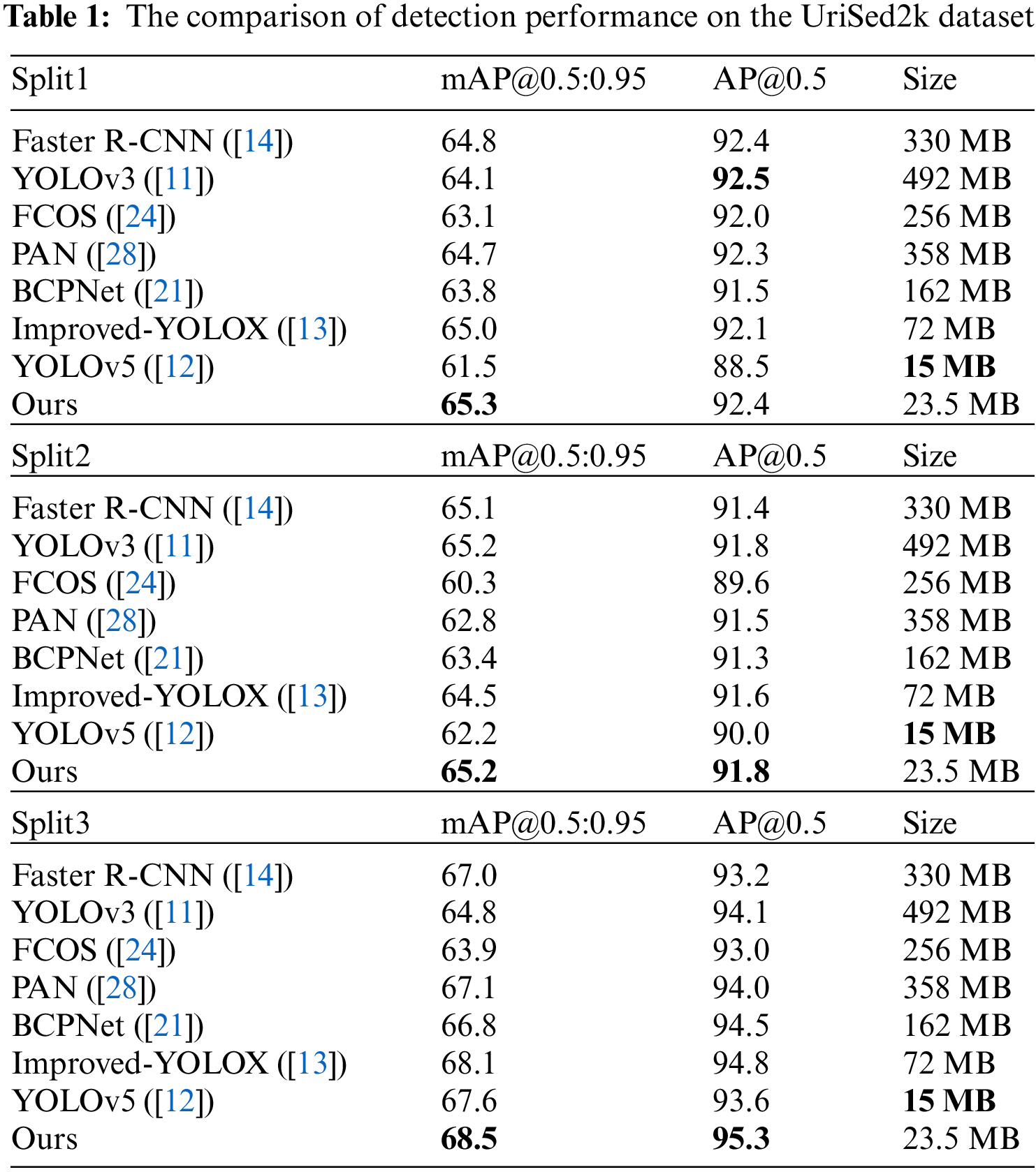
Table 2 compares the detection performance on the UMID dataset [23]. The UMID dataset labels three types of urine sediment, RBCs, WBCs, and epithelial cells. Besides, there are many urine sediments in the images that are not labeled. Despite these situations, we can see from the table that our method performs better on this dataset compared to other methods.

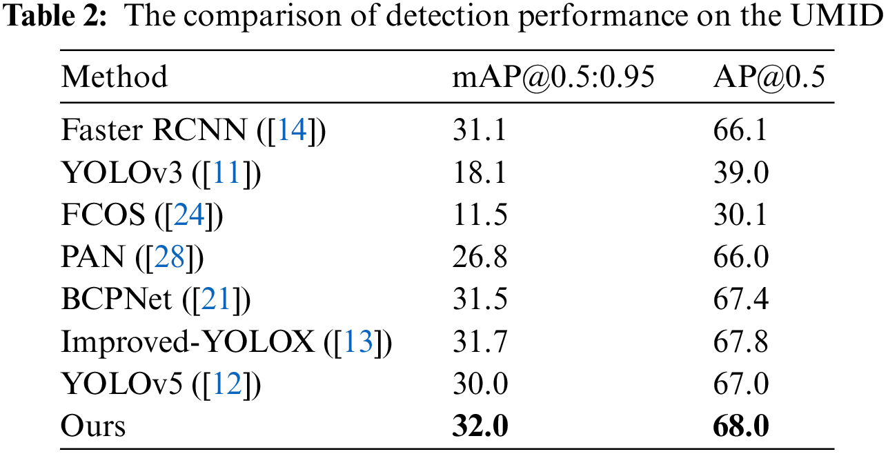
Fig. 7 shows some samples to demonstrate the effectiveness of our approach. We visualize the ground truth and the prediction boxes of each method overlaid onto the original images. When urine sediments are sparsely distributed and not occluded, our method performs almost as well as commonly used object detection methods. In addition, in the case of dense local occlusion, our method is able to more effectively distinguish these particles from the whole part.

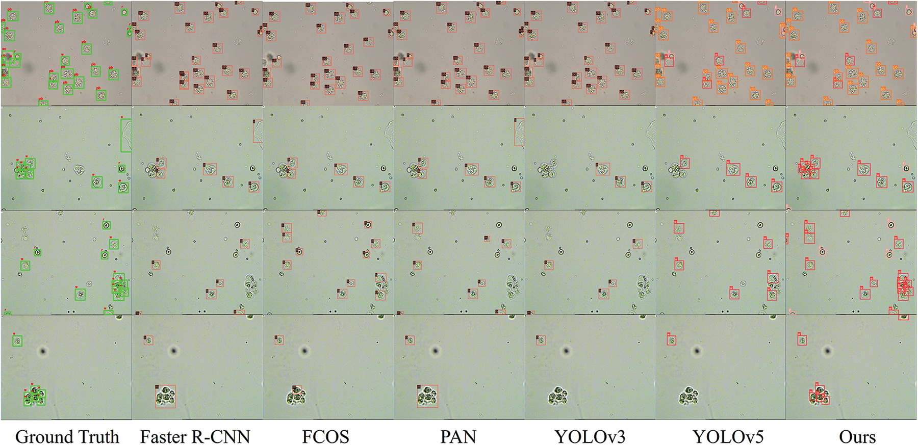
Figure 7: The ground truth and prediction of each method

5.3 Ablation Study

To validate the effectiveness of each component in our proposed method, we conducted ablation experiments on the UriSed2K dataset. The baseline model used was a small YOLOv5 object detector without the local context attention (LCA) module and the global background suppression (GBS) module. Table 3 shows two overall metrics and the precision of the seven classes of urine sediment particles at the IoU of 0.5. Our results demonstrate that the addition of the LCA and GBS modules significantly improves the precision of the seven types of particles. Overall, our results show that our proposed method effectively works on the urine sediment dataset.

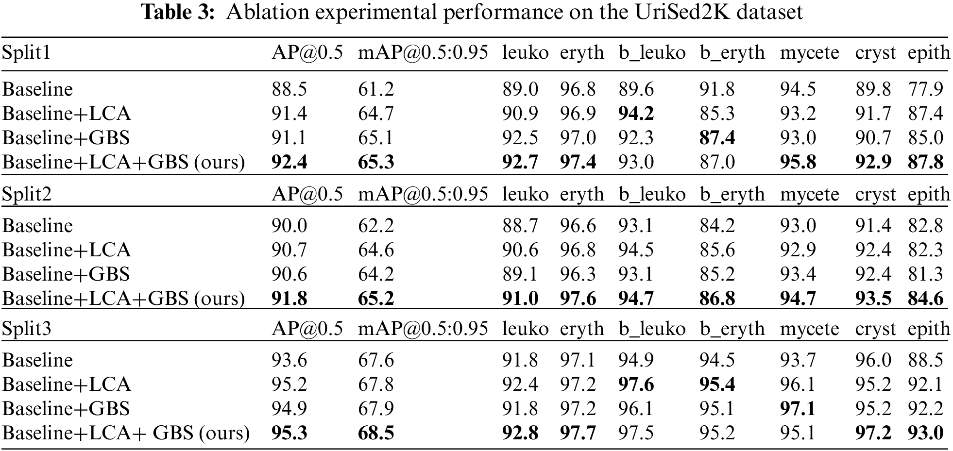
Fig. 8 shows the heat maps detected by four network models, reflecting where the network focuses. Each heat map is generated based on the convolutional output of the last layer of the network. Specifically, the calculation method is to normalize the predicted objectness scores for each position to between 0 and 1, then map them onto a heat map of the same size as the input image. This allows us to judge the degree of network attention to different areas based on the color of each position. These heat maps have a gradient of colors from blue to red, with darker red areas indicating more attention from the network.

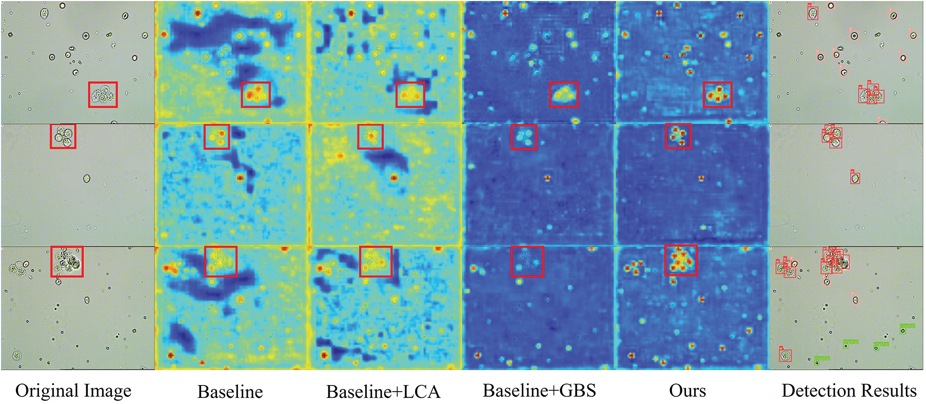
Figure 8: We show three examples of local densities highlighted by red boxes. The heat maps are visualized to origin images by four network modules. The baseline is small YOLOv5 [12]. The local context attention (LCA) module and global background suppression (GBS) module are our proposed methods. From the detection results, we see that the objects in the red boxes are well separately detected

The heat maps in the third column demonstrate the effectiveness of our LCA module in capturing context information. This enables the model to increase its perception of information surrounding particles, thus effectively separating locally dense particles. However, we also notice that the LCA module can overly focus on the background, which is redundant. This is where the GBS module comes in, as it suppresses the model’s attention to the background. The heat maps in the fourth column show how the GBS module helps the model focus less on the background. Overall, the LCA and GBS modules work together to help the model deal with local density and global sparsity in urine sediment detection. In Fig. 9, we can clearly see which categories the objects were predicted to belong to. Our improved method has significantly improved the detection recall rate compared to the baseline, and the accuracy of most categories has also improved.

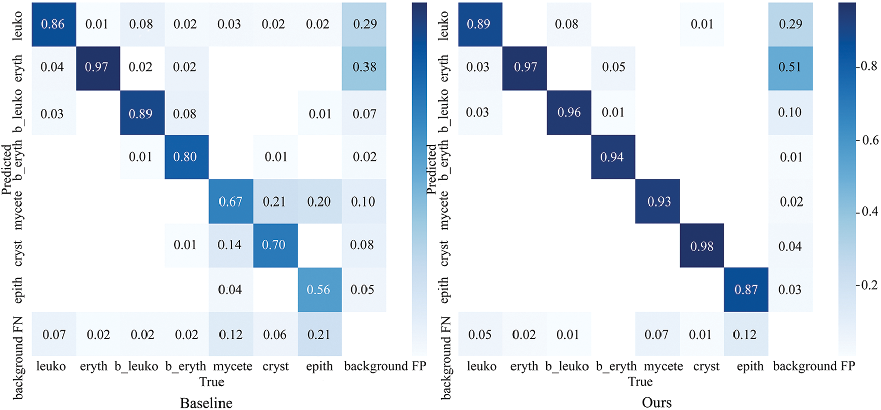
Figure 9: The confusion matrix. The values in each cell of the confusion matrix are normalized to a range between 0 and 1. The values on the diagonal represent the recall rate of the predicted category. The accuracy of the prediction can be calculated by dividing the value on the diagonal by the sum of the corresponding row

6  Conclusion

This manuscript presented a urine sediment dataset called UriSed2K containing 2465 images with a total of 29450 instances. We proposed the improved method of discriminatory-YOLOv5s. It was a lightweight network model with two effective modules, the local context attention (LCA) module and the ground background suppression (GBS) module, for object detection on urine sediment images. The LCA module enhanced the model’s perception ability by capturing context information around the targets. The GBS module suppressed the model’s attention to the background, therefore enabling the model to concentrate on the locations with features. These two modules, proposed for the main challenges of the urine sediment dataset, obviously improved the detector’s performance in small objects and got the best average precision of 95.3% at IoU = 0.5. Our dataset will contribute to object detection and recognition in urine sediment images. The UriSed2K dataset enables the development of automated urinalysis techniques, which reduces the time and labor costs associated with manual analysis and improves the accuracy and efficiency of analyses. Analyzing urine sediment datasets can provide insights into changes in urine sediments in different diseases or pathological states, and can offer valuable data support for related medical research. Our method can be combined with automatic urine sediment analyzers to obtain real-time counts of various urine sediment particles in images. This allows medical professionals to save time and analyze samples more efficiently, ultimately aiding in the diagnosis of medical conditions. Our method still requires many images to obtain detection performance, and there are many different forms of urine sediment in the images, which are difficult to label. There is great potential to apply this dataset in few-shot detection to reduce annotation efforts.

Acknowledgement: The authors would like to thank the anonymous reviewers and the editors of the journal. Your constructive comments have improved the quality of this paper.

Funding Statement: This work was partially supported by the National Natural Science Foundation of China (Grant Nos. 61906168, U20A20171), Zhejiang Provincial Natural Science Foundation of China (Grant Nos. LY23F020023, LY21F020027), Construction of Hubei Provincial Key Laboratory for Intelligent Visual Monitoring of Hydropower Projects (Grant Nos. 2022SDSJ01).

Author Contributions: The authors confirm contribution to the paper as follows: data collection: Hongqiang Wang; study conception and design: Sixian Chan, Binghui Wu; coding, experimental evaluation: Binghui Wu; analysis and interpretation of results: Binghui Wu, Guodao Zhang; funding support: Sixian Chan, Hongqiang Wang, Yuan Yao; draft manuscript preparation: Guodao Zhang, Yuan Yao; draft review: Binghui Wu. All authors reviewed the results and approved the final version of the manuscript.

Availability of Data and Materials: The dataset UriSed2K that supports the findings of this study is publicly available from https://github.com/binghuiwu98/discriminatory-yolov5. The dataset UMID is publicly available from [23].

Conflicts of Interest: The authors declare that they have no conflicts of interest to report regarding the present study.

References

1. Lakatos, J., Bodor, T., Zidarics, Z., Nagy, J. (2000). Data processing of digital recordings of microscopic examination of urinary sediment. Clinica Chimica Acta, 297(1–2), 225–237. [Google Scholar]

2. Davis, R., Jones, J. S., Barocas, D. A., Castle, E. P., Lang, E. K. et al. (2012). Diagnosis, evaluation and follow-up of asymptomatic microhematuria (AMH) in adults: AUA guideline. The Journal of Urology, 188(6S), 2473–2481. [Google Scholar] [PubMed]

3. Cavanaugh, C., Perazella, M. A. (2019). Urine sediment examination in the diagnosis and management of kidney disease: Core curriculum 2019. American Journal of Kidney Diseases, 73(2), 258–272. [Google Scholar] [PubMed]

4. Zhang Y., Satapathy S. C., Zhu L. Y., Górriz J. M., Wang S. (2020). A seven-layer convolutional neural network for chest CT-based COVID-19 diagnosis using stochastic pooling. IEEE Sensors Journal, 22(18), 17573–17582. [Google Scholar] [PubMed]

5. Shao, J., Chen, S. (2023). Application of U-Net and optimized clustering in medical image segmentation: A review. Computer Modeling in Engineering & Sciences, 136(3), 2173–2219. https://doi.org/10.32604/cmes.2023.025499 [Google Scholar] [CrossRef]

6. Zhang, G., Navimipour, N. J. (2022). A comprehensive and systematic review of the IoT-based medical management systems: Applications, techniques, trends and open issues. Sustainable Cities and Society, 82(4), 103914. [Google Scholar]

7. Mahajan, S., Abualigah, L., Pandit, A. K. (2022). Hybrid arithmetic optimization algorithm with hunger games search for global optimization. Multimedia Tools and Applications, 81(20), 28755–28778. [Google Scholar]

8. Sun, Q., Yang, S., Sun, C., Yang, W. (2018). An automatic method for red blood cells detection in urine sediment micrograph. 2018 33rd Youth Academic Annual Conference of Chinese Association of Automation (YAC), pp. 241–245. IEEE. [Google Scholar]

9. Ji, Q., Li, X., Qu, Z., Dai, C. (2019). Research on urine sediment images recognition based on deep learning. IEEE Access, 7, 166711–166720. https://doi.org/10.1109/ACCESS.2019.2953775 [Google Scholar] [CrossRef]

10. Wang, S. H., Nayak, D. R., Guttery, D. S., Zhang, X., Zhang, Y. D. (2021). COVID-19 classification by CCSHNet with deep fusion using transfer learning and discriminant correlation analysis. Information Fusion, 68, 131–148. [Google Scholar] [PubMed]

11. Redmon, J., Farhadi, A. (2018). YOLOv3: An incremental improvement. arXiv preprint arXiv:1804.02767. [Google Scholar]

12. Jocher, G., Stoken, A., Borovec, J., Chaurasia, A., Changyu, L. et al. (2021). Ultralytics/yolov5:V5.0-YOLOv5-P6 1280 models, aws, supervisely and youtube integrations. Zenodo. https://doi.org/10.5281/zenodo.4679653 [Google Scholar] [CrossRef]

13. Yu, M., Lei, Y., Shi, W., Xu, Y., Chan, S. (2022). An improved yolox for detection in urine sediment images. Intelligent Robotics and Applications: 15th International Conference, ICIRA 2022, Proceedings, pp. 556–567. Harbin, China, Springer. [Google Scholar]

14. Ren, S., He, K., Girshick, R., Sun, J. (2015). Faster R-CNN: Towards real-time object detection with region proposal networks. Advances in Neural Information Processing Systems, 28, 91–99. [Google Scholar]

15. Everingham, M., van Gool, L., Williams, C. K. I., Winn, J., Zisserman, A. (2010). The pascal visual object classes (VOC) challenge. International Journal of Computer Vision, 88(2), 303–338. [Google Scholar]

16. Deng, J., Dong, W., Socher, R., Li, L. J., Li, K. et al. (2009). ImageNet: A large-scale hierarchical image database. 2009 IEEE Conference on Computer Vision and Pattern Recognition, pp. 248–255. Miami, Florida, IEEE. [Google Scholar]

17. Lin, T. Y., Maire, M., Belongie, S., Hays, J., Perona, P. et al. (2014). Microsoft COCO: Common objects in context. European Conference on Computer Vision, pp. 740–755. Zurich, Switzerland, Springer. [Google Scholar]

18. Wang, S. H., Govindaraj, V. V., Górriz, J. M., Zhang, X., Zhang, Y. D. (2021). COVID-19 classification by FGCNet with deep feature fusion from graph convolutional network and convolutional neural network. Information Fusion, 67, 208–229. [Google Scholar] [PubMed]

19. Velasco, J. S., Cabatuan, M. K., Dadios, E. P. (2019). Urine sediment classification using deep learning. Lecture Notes on Advanced Research in Electrical and Electronic Engineering Technology, 180–185. [Google Scholar]

20. Liang, Y., Kang, R., Lian, C., Mao, Y. (2018). An end-to-end system for automatic urinary particle recognition with convolutional neural network. Journal of Medical Systems, 42(9), 1–14. [Google Scholar]

21. Yan, M., Liu, Q., Yin, Z., Wang, D., Liang, Y. (2020). A bidirectional context propagation network for urine sediment particle detection in microscopic images. ICASSP 2020-2020 IEEE International Conference on Acoustics, Speech and Signal Processing (ICASSP), pp. 981–985. Barcelona, Spain, IEEE. [Google Scholar]

22. Liang, Y., Tang, Z., Yan, M., Liu, J. (2018). Object detection based on deep learning for urine sediment examination. Biocybernetics and Biomedical Engineering, 38(3), 661–670. [Google Scholar]

23. Goswami, D., Aggrawal, H. O., Gupta, R., Agarwal, V. (2021). Urine microscopic image dataset. arXiv preprint arXiv:2111.10374. [Google Scholar]

24. Tian, Z., Shen, C., Chen, H., He, T. (2019). FCOS: Fully convolutional one-stage object detection. Proceedings of the IEEE/CVF International Conference on Computer Vision, pp. 9627–9636. Seoul, Korea (South). [Google Scholar]

25. Zhang, Y. D., Dong, Z., Wang, S. H., Yu, X., Yao, X. et al. (2020). Advances in multimodal data fusion in neuroimaging: Overview, challenges, and novel orientation. Information Fusion, 64, 149–187. [Google Scholar] [PubMed]

26. Lin, T. Y., Dollár, P., Girshick, R., He, K., Hariharan, B. et al. (2017). Feature pyramid networks for object detection. Proceedings of the IEEE Conference on Computer Vision and Pattern Recognition, pp. 2117–2125. Honolulu, HI, USA. [Google Scholar]

27. Rao, Y., Mu, H., Yang, Z., Zheng, W., Wang, F. et al. (2022). B-PesNet: Smoothly propagating semantics for robust and reliable multi-scale object detection for secure systems. Computer Modeling in Engineering & Sciences, 132, 1039–1054. https://doi.org/10.32604/cmes.2022.020331 [Google Scholar] [CrossRef]

28. Liu, S., Qi, L., Qin, H., Shi, J., Jia, J. (2018). Path aggregation network for instance segmentation. Proceedings of the IEEE Conference on Computer Vision and Pattern Recognition, pp. 8759–8768. Salt Lake City, UT, USA. [Google Scholar]

29. Ramachandran, P., Parmar, N., Vaswani, A., Bello, I., Levskaya, A. et al. (2019). Stand-alone self-attention in vision models. Advances in Neural Information Processing Systems 32: Annual Conference on Neural Information Processing Systems (NeurIPS), pp. 68–80. Vancouver, BC, Canada. [Google Scholar]

30. Ren, G., Dai, T., Barmpoutis, P., Stathaki, T. (2020). Salient object detection combining a self-attention module and a feature pyramid network. Electronics, 9(10), 1702. [Google Scholar]

31. Liu, S., Huang, D., Wang, Y. (2019). Learning spatial fusion for single-shot object detection. arXiv preprint arXiv:1911.09516. [Google Scholar]

32. Wang, Q., Wu, B., Zhu, P., Li, P., Zuo, W. et al. (2020). ECA-Net: Efficient channel attention for deep convolutional neural networks. IEEE/CVF Conference on Computer Vision and Pattern Recognition, pp. 11531–11539. Seattle, WA, USA. [Google Scholar]

33. Zheng, Z., Wang, P., Liu, W., Li, J., Ye, R. et al. (2020). Distance-IoU loss: Faster and better learning for bounding box regression. Proceedings of the AAAI Conference on Artificial Intelligence, vol. 34, pp. 12993–13000. New York, NY, USA. [Google Scholar]

34. Neubeck, A., Van Gool, L. (2006). Efficient non-maximum suppression. 18th International Conference on Pattern Recognition (ICPR’06), vol. 3, pp. 850–855. Hong Kong, China, IEEE. [Google Scholar]

35. Chen, K., Wang, J., Pang, J., Cao, Y., Xiong, Y. et al. (2019). MMDetection: Open MMLab detection toolbox and benchmark. arXiv preprint arXiv:1906.07155. [Google Scholar]