Improved STN Models and Heuristic Rules for Cooperative Scheduling in Automated Container Terminals

1  Introduction

Globalization of trade is the trend, and more than 80% of world trade is transported by sea [1]. Automated container terminals (ACTs) provide an important guarantee for the transfer of cargo on ships, so it is significant to improve the service level of ACTs. The ACT is a complex production operation system whose service level is mainly determined by the cooperative efficiency of equipment. Automated guided vehicles (AGVs) play a key role in linking seaside operations with yard-side operations. The container yard where yard cranes (YCs) are located is the largest area and has the most concentrated operations in the ACT. Hence, it is important for the ACT to improve the cooperative efficiency between YCs and AGVs. The cooperative scheduling problem of YCs and AGVs is called “CSPYA” in this paper.

The solution methods for solving the CSPYA can be divided into two categories. The first category is exact solution methods, such as solver [2], branch and bound algorithm [3], and column generation algorithm [4]. The second category is approximate solution methods, for instance, the genetic algorithm (GA) [5–7], the particle swarm optimization algorithm [8,9], and the simulated annealing algorithms [10,11]. In addition, the improvement of GA is also an important topic of research in many studies [12–17]. Optimal solutions can be obtained by exact solution methods; however, this kind of method takes a long time when the scale of the problem is large. In contrast, approximate solution methods that can obtain near-optimal solutions at a faster speed are adopted by many scholars, especially meta-heuristic methods. Global search is performed by meta-heuristic methods to obtain the best paths for YCs and AGVs to complete container tasks, and frequent comparisons are performed to update the best paths in real time. Because of high computational efforts and the complexity of coding and optimization mechanisms, it is difficult for meta-heuristic methods to be widely used in practical production [18]. On the other hand, heuristic rules are used more often by managers in ACTs due to their low computational effort and ease of implementation. Besides, paths that YCs and AGVs will not pass through can be excluded according to heuristic rules, which is very beneficial for speeding up the solution process. Since the focus of this study is to design a method that is easy to implement in programming and has a fast solution speed. By contrast, it seems like heuristic rules are more suitable for this study, so heuristic rules will be designed to try to solve the CSPYA.

Generally, when the results of the scheduling problem are obtained, they are represented in a table or Gantt chart. The sequences of container tasks are often listed in tables, but the information provided is limited. For example, the waiting time for equipment cannot be obtained in [8]. Various movements or stationary periods of the main equipment are displayed by different colored bar charts in Gantt charts. The sequence of container tasks and the status of container tasks at any moment can be known in [19]. Although more information can be provided by Gantt charts, there are still certain limitations, such as the trajectories of the equipment cannot be known. However, all the information provided by the above two methods can be provided by the space-time network (STN). And the cooperative processes of YCs and AGVs to complete tasks and their dynamic movements [20] can also be described by STN. In addition, it was pointed out that the pressure of the horizontal transport area and the waiting time between YCs and AGVs can be reduced by buffers [21,22]. Therefore, STN will be used to solve the CSPYA when buffers are configured on the seaside of the yard.

The rest of the paper is arranged as follows. Section 2 introduces related papers. The problem description is provided and two improved STN models are built in Section 3. The designed method with three groups of heuristic rules and its solution procedures are provided in Section 4. Section 5 is the numerical experiment and the analysis of the results. Conclusions and future directions are provided in Section 6.

2  Related Papers

The conflict problem of YCs and the path planning and collisions of AGVs are the problems to be focused on in the CSPYA. In [9], a dynamic scheduling model for YCs under a balancing strategy was established. In [23], an improved GA was used to solve the constructed mathematical optimization model, considering realistic constraints such as non-crossing between YCs and maintaining a safe distance. Besides, a two-layer GA based on congestion prevention rules was designed to solve the established two-layer planning model in [24]. A model architecture was proposed to modify and optimize the hybrid scheduling problem in [25]. And a chaotic particle swarm optimization algorithm with speed control was designed to obtain near-optimal solutions. In [26], a framework based on the Alternating Direction Method of Multipliers (ADMM) was proposed to decompose the scheduling problem into multiple specific subproblems, and high-quality solutions were obtained by iteration. A simulated annealing particle swarm algorithm was designed to solve the nonlinear mixed integer programming model (MIP) established for multi-device collaborative scheduling optimization in [27]. In some studies, both the conflict problem of YCs and the path planning and collision problems of vehicles were considered in solving collaborative scheduling problems. A hierarchical control architecture and a sequential planning approach were proposed in [28]. In [29], a mixed integer planning model was established with the objective of minimizing the ship’s time in port and minimizing the total energy consumption, and a two-layer GA was designed to acquire solutions. An improved multi-layer GA was designed for solving the collaborative scheduling problem considering buffer zones in a simultaneous loading and unloading operation model in [30].

The safe distance and conflict of YCs for device cooperative scheduling were solved in [22,23], but the path planning and collision avoidance of vehicles were ignored; the path planning and collision avoidance of AGVs for equipment collaborative scheduling were solved in [24–27], but the conflict problem of loading and unloading equipment in the container yard was not considered. In [28–30], the collisions of YCs were avoided by making them operate in fixed blocks. However, one YC usually serves at least one block [31], and results show that YCs are more efficient in flexible operation mode than fixed operation mode [20], so it is more practical to consider YCs in flexible operation mode.

For cooperative scheduling problems that consider simultaneous loading and unloading and buffers. In [32], a model was developed with the objective of minimizing the loading and unloading time of the ship, and the hybrid algorithm of GA and particle swarm optimization was designed. In [33], a dual-objective optimization model with the objective of minimizing the overall operation time and energy consumption was established, and a heuristic-based GA was designed considering the allocation of the storage space. In [34], an integrated optimization model was established, and a GA-based heuristic algorithm was designed to obtain high-quality solutions in a relatively short time. In [35], a model of the multi-device collaborative scheduling problem was developed, which is in the form of a hybrid flow shop, and the model is solved by the simulated annealing algorithm. The improved GA designed in [36] can obtain the approximate optimal solution or optimal solution of the equipment allocation and scheduling problem in a shorter time. In [37], the integrated scheduling problem was formulated as a blocking mixed-flow shop scheduling problem with the bidirectional flow and finite buffers. A mixed-integer linear programming model was developed, and an adaptive large-neighborhood search algorithm was designed to solve it.

Although loading and unloading synchronization as well as buffers were considered in [32–34], no buffer capacity was considered. Although both loading and unloading and the buffer capacity were considered in [35–37], the collision problem of YCs was ignored.

The STN has a significant advantage in describing the trajectory of the device’s movements. In [2], the STN was used to describe the trajectories of two automated stacking cranes (ASCs) in the same block, and the interference between ASCs was analyzed by the time interval between tasks. In [38], an AGV path optimization model was built based on the set of available road segments under the STN, and paths satisfying collision avoidance and congestion mitigation conditions were obtained by iterative updates. In [39], a space-time flow diagram was constructed for the collaborative scheduling problem of multiple devices. Although the STN was used to describe the operations of the devices, the corresponding STN model was not built. In [20], the STN was used to define and describe various motions of YCs and AGVs, and an integer linear programming model M1 in the form of the STN was built.

Only one type of equipment was considered in [2,38]. Although the path planning and conflict problems of devices were considered in [20,39], buffers were not considered. The CSPYA with limited buffer capacity is further studied in this paper and the corresponding STN model is established.

Heuristic rules are often used to quickly obtain feasible solutions to a problem and are frequently used in the study of equipment scheduling problems. In [40], a heuristic method was designed to solve the established MIP model of the automated lifting vehicle scheduling problem in a faster way. In [41], AGVs were considered as ant-agents, and an AGV control method based on the state transition rule and a solution mechanism for node conflicts and path congestion were designed to solve the problem. In [42], a heuristic method was designed to get the schedule of cranes for the integrated scheduling problem. In [43], the collisions of AGVs at intersections were considered when solving the collaborative scheduling problem in the ACT. Then compatible and conflicting phases were set, and results showed that the collisions of AGVs can be effectively reduced by considering collision avoidance rules. A greedy insertion heuristic was designed in [21], and the complete task sequence and completion time (CT) can be obtained quickly for the integrated scheduling problem of quay cranes (QCs), AGVs, and YCs in the unloading process.

Only one kind of equipment was considered in [40,41]. The buffers and conflicts among equipment were not considered in [42]. Only the unloading process was considered in [21,43]. In this paper, the problem of conflict-free cooperative scheduling of equipment with limited buffer capacity in loading and unloading synchronous operation mode is studied.

The focus of this paper is to improve the existing STN model M1 and further apply it to a situation where buffers in the seaside of each block are considered. Two groups of constraints in M1 are improved from the perspective of constraint decomposition. Then the improved STN model is compared with M1 to verify its disadvantages. A heuristic method including the task matching rules of the YC and the AGV, the conflict control rules of the AGV and the waiting rules of the AGV is designed in order to acquire an approximate optimal solution quickly. To test the effectiveness of the proposed method and study the influence of the buffers and the number of blocks on the AGV, corresponding comparative experiments are designed, respectively.

3  Cooperative Scheduling Model

The CSPYA is a complex problem since it is necessary to consider not only the cooperation and restrictions between the YC and the AGV but also the collision between AGVs. The STN has obvious advantages in describing the moving processes of the YC and the AGV; therefore, constraints in the actual operation process are converted into mathematical expressions in the form of the STN. And then, the models STN_A and STN_B are established.

3.1 Problem Description

Handling equipment of the ACT is assigned tasks according to the stowage plans of ships prior to operation in order to make efficient use of limited resources. The buffers configured on the seaside of each block can weaken the coupling relationship between the YC and the AGV, and improve their flexibility and utilization. When an inbound container task is loaded on an AGV, it does not need to wait for the YC if there is an available buffer near the target block. Similarly, a YC does not need to wait for the AGV when a buffer is occupied by an inbound container task. This paper focuses on the CSPYA, which considers limited buffers in the ACT and loading and unloading operations simultaneously. The specific layout of an ACT equipped with buffers is shown in Fig. 1.

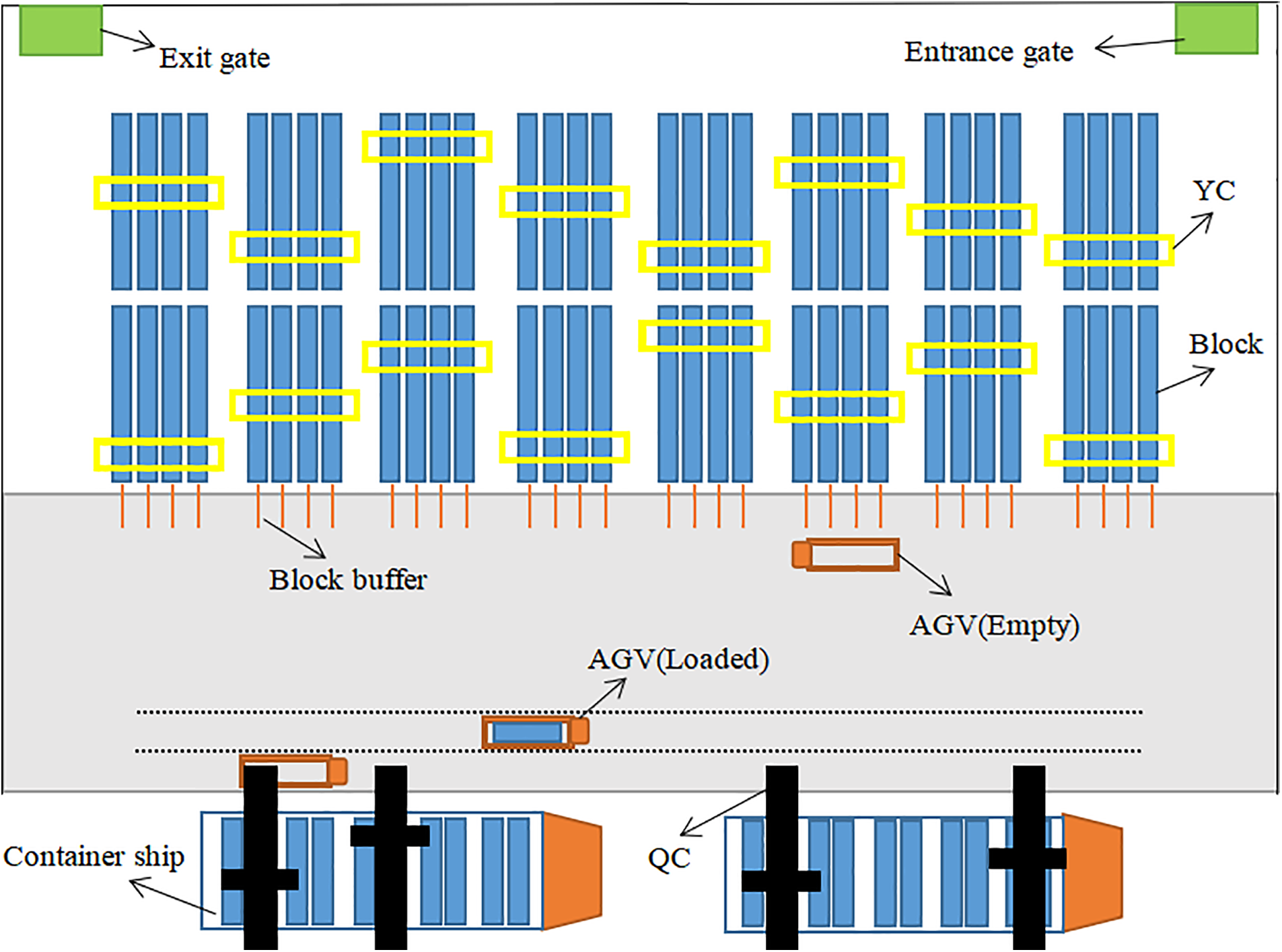
Figure 1: Layout of ACT with buffers

As the loading and unloading processes are similar, the operation behaviors of equipment in the unloading stage are illustrated here as an example. To start with, AGVs carry container tasks from QCs to the buffers of the target block or work directly with YCs to complete container tasks if there is an available buffer. Otherwise, AGVs need to wait for an idle buffer. Then, AGVs return to QCs to carry the rest of the container tasks after container tasks are unloaded from them. Next, YCs extract container tasks from buffers and deposit them at target locations in the yard. Finally, YCs return to the seaside of the yard and continue to extract container tasks from buffers until all container tasks are placed at their target locations.

The tasks of this paper are to make the task matching plan and path planning of the YC and the AGV to minimize the total turn time of the AGV during the entire loading and unloading process.

3.2 Space-Time Network Model

Reasonable assumptions are necessary and they are helpful to analyze and solve the problem due to the complexity of the CSPYA. The definitions of relevant notations are given before modeling. On this basis, the method of describing the CSPYA with STN is introduced in detail. Then, the models STN_A and STN_B are provided.

3.2.1 Assumptions

Considering the complexity of the CSPYA in reality, the following assumptions are made to simplify the problem:

a)   The sequence in which QC operates container tasks is known;

b)   The initial and target positions of loading and unloading container tasks are known;

c)   All equipment can only operate one container task at a time and the operation time is known;

d)   The moving times of the YC and the AGV between any two feasible nodes are known;

e)   The buffer capacity of each block on the seaside of the yard is the same;

f)   It takes the same and constant time for YCs to perform the same type of container tasks;

g)   The time required for unloading a container task from AGVs to a buffer is the same and fixed as the time required for loading a container from a buffer to an AGV.

3.2.2 Notations

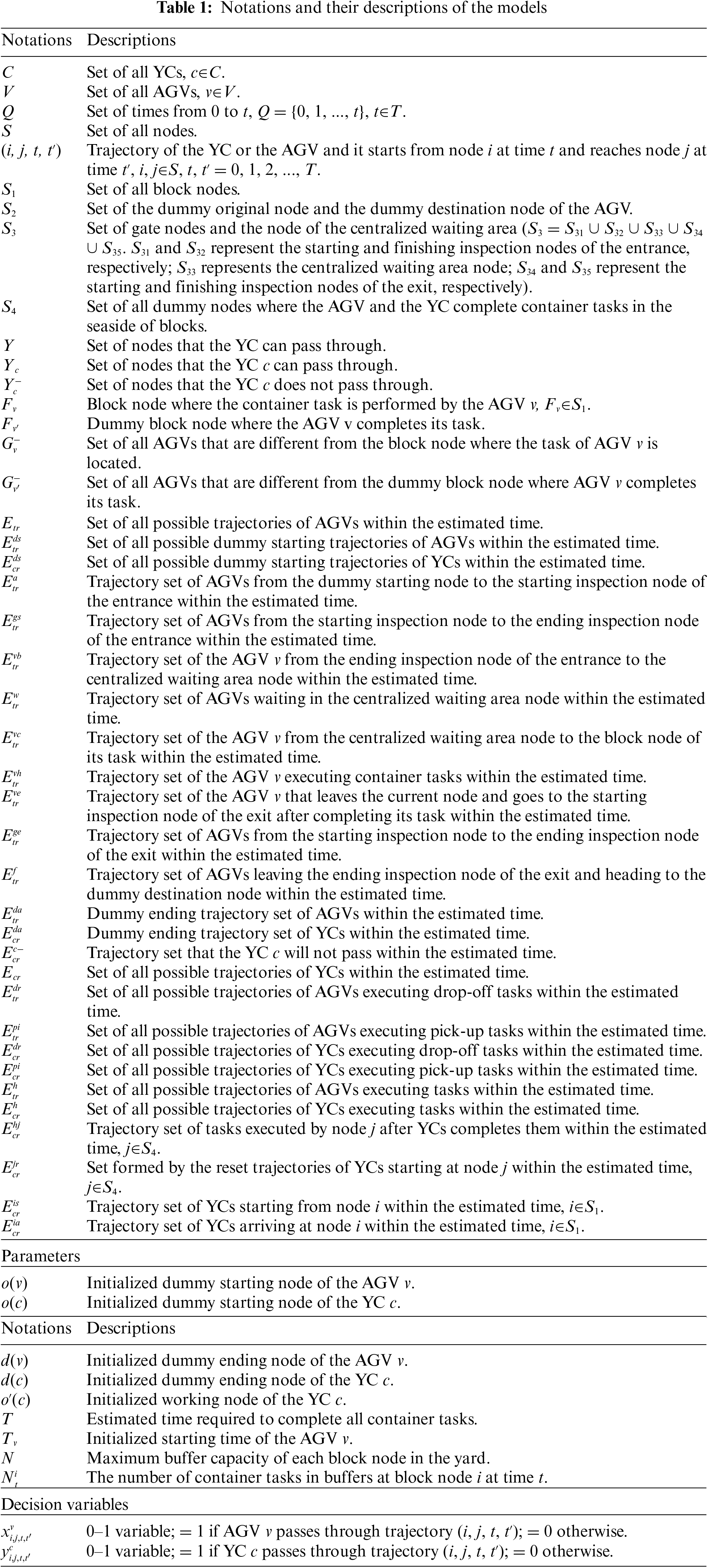
The defined notations and their meanings in the original STN model remain unchanged. Here are the definitions of the parameters used in this paper and some of them are newly added after the buffers are considered. The details are shown in Table 1.

3.2.3 Space-Time Network

Since the AGV and the YC are at different spatial heights, there is no possibility of collision between the two devices, so the same STN can be used to describe the operation processes of the YC and the AGV at the same time. Actions related to the YC and the AGV are described in the form (i, j, t, t′) in the STN, where i and t respectively represent the starting node and starting time of an action, and j and t′ respectively represent the ending node and ending time of the action. Both the YC and the AGV have five types of actions, and four of them are the same, namely “waiting”, “moving”, “pick-up” and “drop-off”. The other action of the YC is “recovery”, and it is used to describe how the spreader of the YC needs to be reset after performing a pick-up or drop-off operation. The other action of the AGV is “inspection”, which describes the process of the AGV being inspected at the gates of the yard. Different from other actions, when the STN is used to describe waiting actions, i = j, which means that the YC or the AGV has not moved in the time period from t to t′. In order to simplify the diagram, each block of the yard and its buffers are regarded as the same node.

Fig. 2 is taken as an example to explain how the actions of the YC and the AGV are described by the STN. The blue line with the arrow and the red line with the arrow depict the movements of the AGV and the YC, respectively. As for YC 2, it is stationary for the first 20 s at node 140, and then it takes 10 s to move from node 140 to node 120; next, it takes 20 s to complete a drop-off task from node 120 to node 122 and then it takes 10 s to return to node 120. Then, the subsequent actions are similar to those described above. As for AGV 3, it is static at node 0 until the 40 s and it spends no time on the movement from node 0 to node 10 because node 0 is a virtual starting node; next, it spends 5 s on gate inspection before entering the yard from node 10 to node 11 and it spends 5 s on the movement from node 11 to node 100; then, it takes 10 s to move from node 100 to node 120 and completes a pick-up task unloaded by the YC 2 within 60~80 s. The YC and the AGV must work together to complete container tasks when there are no buffers. However, the behaviors of the YC and the AGV become different if there are buffers. For instance, the container task can be directly unloaded into a buffer when AGV 1 reaches the target block node, and YC 1 does not need to work with it.

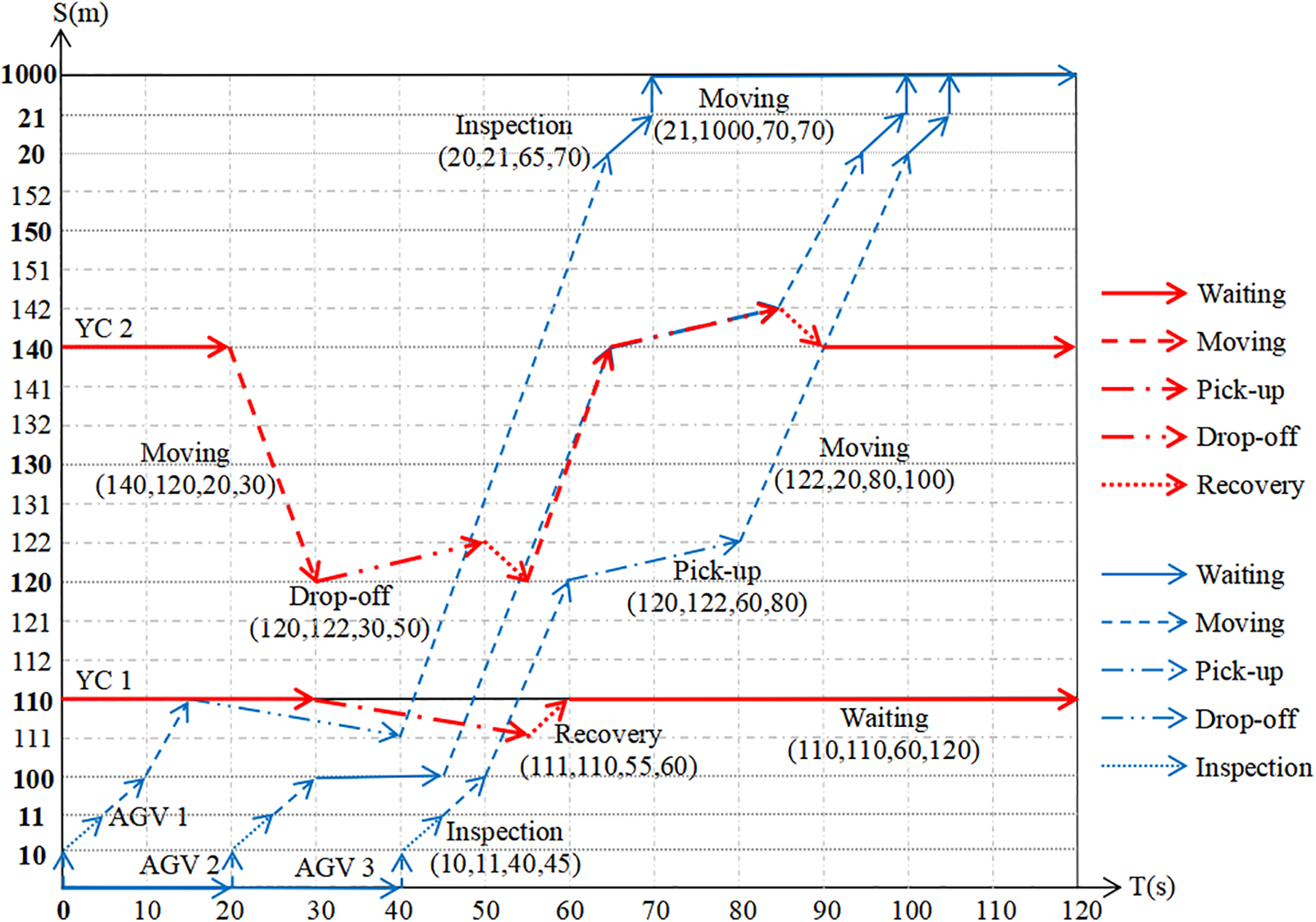
Figure 2: Behavior description of AGV and YC in the STN

The STN can also be used to analyze the occupied status of the buffers. Taking the buffer capacity is 2 as an example, Fig. 2 shows that only buffers at nodes 110, 120, 130, 140, and 150 are occupied in the period of 0~120 s. One buffer at node 110 is occupied by AGV 1 at 15 s; the buffers at node 110 are idle after 55 s because YC 1 just completes the container task. Besides, there is only one idle buffer at node 140 within the 65~85 s since YC 2 and AGV 2 are working together to complete the container task; by 85 s, YC 2 completes the container task and its spreader begins to reset; AGV 2 begins to leave node 140 at 85 s, and then the buffers at this node are idle. It should be noted that AGV 2 does not move after reaching a buffer at node 140 in the actual operations. The action (140, 142, 65, 85) corresponding to AGV 2 is intended to show the cooperative relationship between AGV 2 and YC 2.

3.2.4 Improved Space-Time Network Models

The definition domains of decision variables are divided into different sets according to their paths at different nodes and these sets are defined separately. Then the flow balance constraints in M1 are decomposed into Eqs. (1)–(15). This can speed up the solution process because CPLEX solves the decomposed formulas by searching the paths from the corresponding sets each time instead of searching the whole definition domain. In addition, the trajectories of YCs and AGVs can be further constrained according to the task type and operation mode of the equipment, which helps to further accelerate the solution process. Eqs. (16)–(18) are added trajectory constraints. STN_A is composed of Eqs. (1)–(18) and constraints in M1, except the flow balance constraints. The Eqs. (1)–(18) are as follows:

xi,j,t,t′v=1,i=j=o(v),t=0,t′=Tv, ∀v∈V(1)

∑(i,j,t,t′)∈Etrdsxi,j,t,t′v=1, ∀v∈V(2)

∑i,t:(i,j,t,t′)∈Etraxi,j,t,t′v=∑i,t:(j,i,t′,t)∈Etrdsxi,j,t,t′v, ∀v∈V(3)

∑i,t:(i,j,t,t′)∈Etrgsxi,j,t,t′v=∑i,t:(j,i,t′,t)∈Etraxi,j,t,t′v, ∀v∈V(4)

∑i,t:(i,j,t,t′)∈Etrvc∪Etrwxi,j,t,t′v=∑i,t:(j,i,t′,t)∈Etrgs∪Etrwxi,j,t,t′v, ∀v∈V(5)

∑i,t:(i,j,t,t′)∈Etrvhxi,j,t,t′v=∑i,t:(j,i,t′,t)∈Etrvcxi,j,t,t′v, ∀v∈V(6)

∑i,t:(i,j,t,t′)∈Etrvexi,j,t,t′v=∑i,t:(j,i,t′,t)∈Etrvhxi,j,t,t′v, ∀v∈V(7)

∑i,t:(i,j,t,t′)∈Etrgexi,j,t,t′v=∑i,t:(j,i,t′,t)∈Etrvexi,j,t,t′v, ∀v∈V(8)

∑i,t:(i,j,t,t′)∈Etrfxi,j,t,t′v=∑i,t:(j,i,t′,t)∈Etrgexi,j,t,t′v, ∀v∈V(9)

∑i,t:(i,j,t,t′)∈Etrdaxi,j,t,t′v=∑i,t:(j,i,t′.t)∈Etrfxi,j,t,t′v, ∀v∈V(10)

yi,j,t,t′c=1,i=o(c),j=o′(c),t=0,t′=1,∀c∈C(11)

∑t:(i,j,t,t′)∈Ecrisyi,j,t,t′c−∑t:(j,i,t′,t)∈Ecriayj,i,t′,tc=0, ∀i∈S1,c∈C(12)

∑t′:(i,j,t,t′)∈Ecrhjyi,j,t,t′c−∑t′:(j,i,t′,t)∈Ecrjryj,i,t′,tc=0, ∀j∈S4,c∈C(13)

∑(i,j,t,t′)∈Ecrdayi,j,t,t′c=1, ∀j=o′(c),c∈C(14)

∑(i,j,t,t′)∈Ecrdsyi,j,t,t′v=1, ∀c∈C(15)

∑(i,j,t,t′)∈Etrvcxi,j,t,t′v=0, ∀v∈Gv−(16)

∑(i,j,t,t′)∈Etrvhxi,j,t,t′v=0, ∀v∈Gv′−(17)

∑i,t:(i,j,t,t′)∈Ecrc−yi,j,t,t′c=0, ∀c∈C(18)

Eq. (1) determines the virtual starting trajectory of the AGV according to the departure time. Eq. (2) guarantees the uniqueness of the virtual starting trajectory for each AGV. Eqs. (3)–(10) ensure that the number of the trajectory of any AGV reaching node i at time t is equal to the number of the trajectory starting from this node. Therefore, the continuity of AGV movements between different nodes is ensured. Eq. (11) determines the virtual starting trajectory of each YC based on its departure time. Eq. (12) ensures that the number of trajectories arriving at the block node i at time t equals the number of trajectories departing from the node at that time. Eq. (13) guarantees that the number of trajectories arriving at the task completion node j at time t′ equals the number of trajectories departing from the node at that time. Eqs. (12) and (13) are integrated to ensure the continuity of the YC’s operations. Eq. (14) guarantees that the YC eventually reaches the virtual ending node. Eq. (15) ensures the unique virtual starting path of each YC. Eqs. (16) and (17) eliminate trajectories that the AGV will not pass based on container tasks. Eq. (18) determines the trajectories that each YC will not pass due to its operating interval.

Moreover, the STN model is further extended to solve the CSPYA with buffers on the seaside of the yard. Because the cooperative relationship between the AGV and the YC has changed after the buffers were added, the coupling constraint in the STN_A is replaced by Eqs. (19) and (20). On the basis of the above, the Eqs. (21)–(32) on buffers are added and this yields STN_B. Eqs. (19)–(32) are as follows:

∑v∈V∑i:(i,j,t,t′)∈Etrdrxi,j,t,t′v=∑c∈C∑i:(i,j,t,t′)∈Ecrpiyi,j,t,t′c, ∀i∈S(19)

∑v∈V∑i:(i,j,t,t′)∈Etrpixi,j,t,t′v=∑c∈C∑i:(i,j,t,t′)∈Ecrdryi,j,t,t′c, ∀i∈S(20)

Nti≤N(21)

0≤Nti+∑v∈V∑i:(i,j,t,t′)∈Etrdrxi,j,t,t′v−∑v∈V∑i:(i,j,t,t′)∈Etrpixi,j,t,t′v+∑c∈C∑i:(i,j,t,t′)∈Ecrdryi,j,t,t′c−∑c∈C∑i:(i,j,t,t′)∈Ecrpiyi,j,t,t′c≤N, ∀i∈S(22)

0≤Nti+∑v∈V∑i:(i,j,t,t′)∈Etrdrxi,j,t,t′v≤N, ∀i∈S(23)

0≤Nti−∑v∈V∑i:(i,j,t,t′)∈Etrpixi,j,t,t′v≤N, ∀i∈S(24)

0≤Nti+∑c∈C∑i:(i,j,t,t′)∈Ecrdryi,j,t,t′c≤N, ∀i∈S(25)

0≤Nti−∑c∈C∑i:(i,j,t,t′)∈Ecrpiyi,j,t,t′c≤N, ∀i∈S(26)

0≤Nti+∑v∈V∑i:(i,j,t,t′)∈Etrdrxi,j,t,t′v+∑c∈C∑i:(i,j,t,t′)∈Ecrdryi,j,t,t′c≤N, ∀i∈S(27)

0≤Nti+∑v∈V∑i:(i,j,t,t′)∈Etrdrxi,j,t,t′v−∑c∈C∑i:(i,j,t,t′)∈Ecrpiyi,j,t,t′c≤N, ∀i∈S(28)

0≤Nti−∑v∈V∑i:(i,j,t,t′)∈Etrpixi,j,t,t′v+∑c∈C∑i:(i,j,t,t′)∈Ecrdryi,j,t,t′c≤N, ∀i∈S(29)

0≤Nti−∑v∈V∑i:(i,j,t,t′)∈Etrpixi,j,t,t′v−∑c∈C∑i:(i,j,t,t′)∈Ecrpiyi,j,t,t′c≤N, ∀i∈S(30)

∑v∈V∑t∈Qxi,j,t,t′v−∑c∈C∑t∈Qyi,j,t,t′c≥0, ∀(i,j,t,t′)∈Etrdr(31)

∑c∈C∑t∈Qyi,j,t,t′c−∑v∈V∑t∈Qxi,j,t,t′v≥0, ∀(i,j,t,t′)∈Etrpi(32)

Eq. (19) ensures that the number of tasks unloaded from the AGV on buffers of any block node is equal to the number of tasks extracted from buffers of the same node by the YC. Eq. (20) ensures that the number of tasks loaded on the AGV from buffers of any block node equals the number of tasks unloaded on buffers of the same node by the YC. Eq. (21) ensures that the number of containers in any buffer at any time does not exceed N. Eqs. (22)–(30) ensure that operations on containers starting from t in any buffer need to meet the capacity limit. Eqs. (31) and (32) represent actual constraints on the YC and the AGV to perform container tasks. An AGV must have performed a drop-off task on a node before a YC executes a pick-up task on the node. And a YC must have performed a drop-off task on a node before an AGV executes a pick-up task on the node.

4  Heuristic Rules

A feasible solution to complex scheduling problems can be obtained by heuristic methods within a relatively short time. In order to obtain higher-quality feasible solutions or even the optimal solution, it is necessary to design suitable rules according to practical problems. Three groups of heuristic rules are designed, and the steps for using them to solve the CSPYA are introduced in this section.

4.1 Design of the Heuristic Rules

Three groups of heuristic rules are designed. Task matching rules are designed to match AGVs with YCs quickly. The conflict control rules designed for AGVs are used to resolve conflicts when they enter or leave the yard gates. The waiting rules for AGVs are used to prevent congestion and blockages on the roads.

4.1.1 Task Matching Rules

The AGV and the YC work together based on the working range of the YC and the node where the tasks of the AGV will be performed. All tasks are completed by them according to the times that AGVs arrive at the block nodes. The AGV closest to the YC is selected by the YC to complete the task if many AGVs arrive at the nodes within the YC’s working range at the same time. Moreover, an AGV is randomly selected by the YC to collaborate with it if two or more AGVs arrive at the nodes at the same distance from the node where the YC is located.

4.1.2 Conflict Control Rules

The strategy with the lowest cost for controlling the AGVs is selected when conflicts occur at the entrance or exit of the yard; the strategy with the least number of AGVs is selected when the cost of controlling the AGVs is the same; one of the strategies is selected randomly when the cost of controlling the AGVs is the same and the number of AGVs that need to be controlled is the same.

Six common conflict types and corresponding AGV control strategies are depicted in Fig. 3 when the gate into or out of the yard is two-lane and the gate inspection time is three time units. The number of AGVs is represented by the number in the circle. The expected arrival of an AGV is represented by the blue circle and the AGV that needs to control speed is represented by the red circle. The specific conflict situations are shown in the first line of Figs. 3a–3f. The control strategies to resolve conflicts among AGVs are represented by the rows from the second to the last, and the priority of the strategies decreases from top to bottom. Moreover, the cost of AGVs under the corresponding control strategy is represented by the number next to the right arrow. Fig. 3a is taken as an example to illustrate the selection process of AGV control strategies. The first AGV control strategy is preselected when the conflict occurs, and then it is checked whether the adoption of this strategy will cause subsequent conflicts. If the adoption of the first AGV control strategy will not cause subsequent conflicts, the adoption of this strategy is determined. Otherwise, throw out the preselected AGV control strategy and switch it out for the second AGV control strategy before repeating the selection procedure. The first AGV control strategy is selected if it is found that all control policies have subsequent conflicts. Next, the subsequent conflicts caused by the adoption of this strategy will be determined. Then, the corresponding AGV control strategy is selected in Fig. 3 according to the above steps.

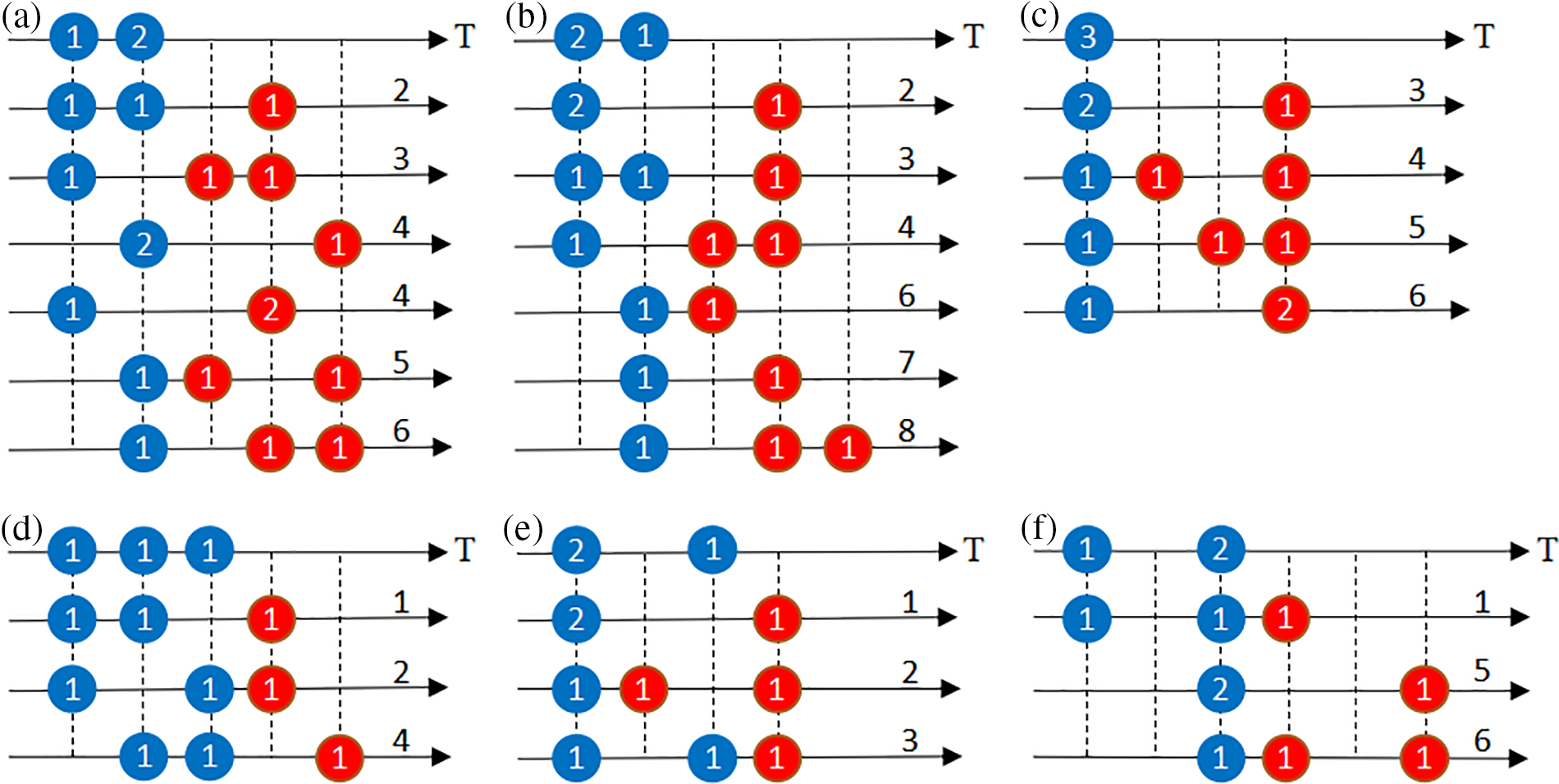
Figure 3: Six conflict types and corresponding control rules for AGV

4.1.3 Waiting Rules

The working state of the YC corresponding to an AGV can be obtained according to the starting time of the AGV. Then, whether the current AGV needs to enter the centralized waiting area node can be determined. There are two scenarios. The AGV does not need to enter the node if the YC matched with it can arrive at the target node before or simultaneously with the AGV. Otherwise, the AGV needs to enter the node. And the waiting time (WT) of the AGV is based on both the working state of the YC that is cooperating with it and the time required for the YC to move from the current node to the target node.

4.2 Solving Process

The method with three groups of heuristic rules is designed to solve the CSPYA; the flowchart of the method is shown in Fig. 4. For the convenience of explanation, the container task of AGV v is defined as Taskv, and M is a large constant. It is necessary to ensure that all tasks can be completed by the YC and the AGV within M min. In addition, the task matching rules, the conflict control rules, and the waiting rules are denoted as Rule 1, Rule 2, and Rule 3, respectively. The specific steps are as follows:

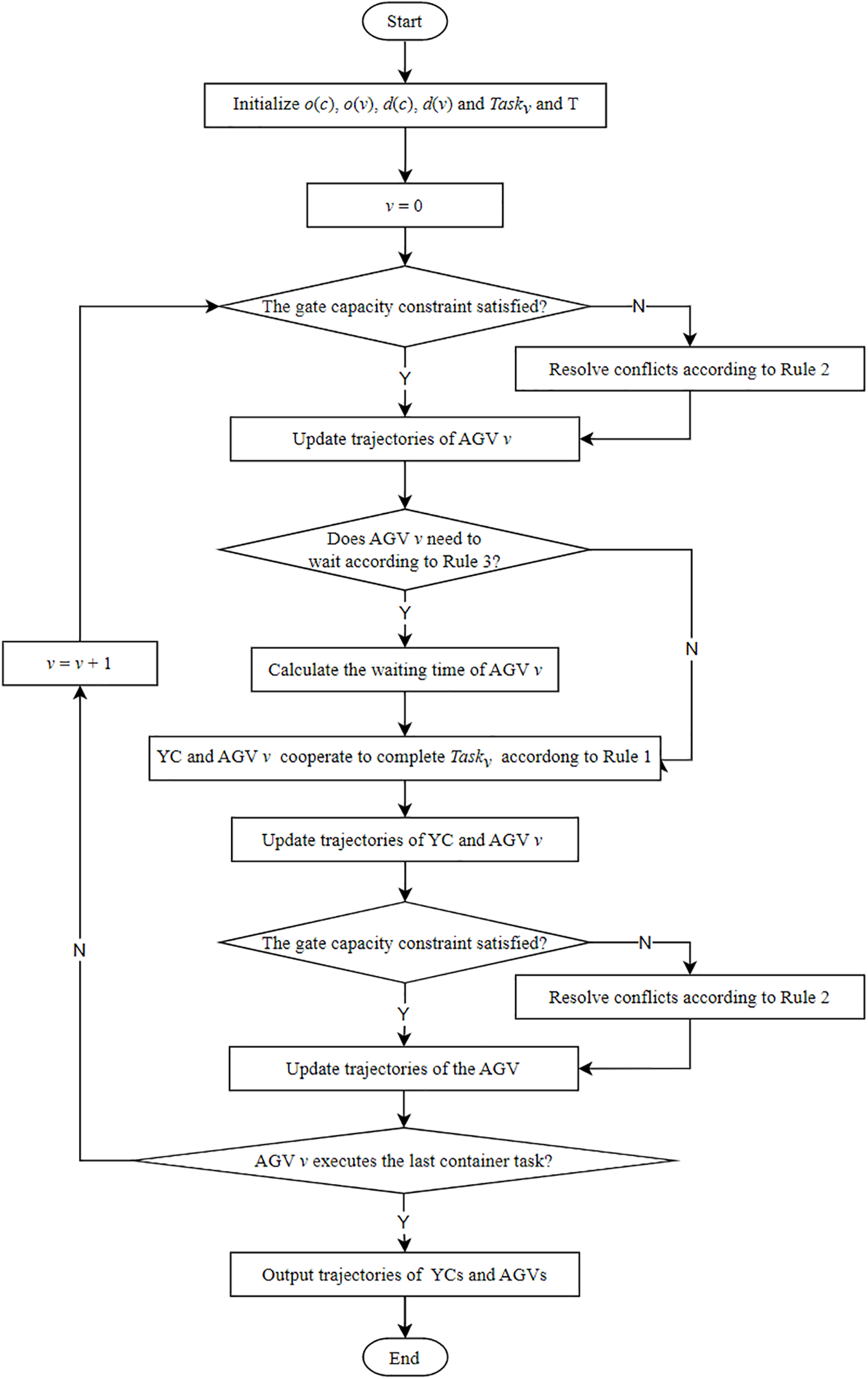
Figure 4: Flowchart of the heuristic method

Step 1: Initialization. Initialize o(c) = o(v) = 0, d(c) = o′(c), d(v) = 1000, Taskv = (Fv, Fv’), T = M.

Step 2: v = 0.

Step 3: Judge if the gate capacity constraint is satisfied when AGV v enters the yard. If yes, the trajectories are directly updated; otherwise, the trajectories are updated after the conflict is resolved according to the Rule 2.

Step 4: Determine whether AGV v needs to enter the centralized waiting area node according to the Rule 3. If it needs to wait, the waiting time is determined according to the working state of the YC that is collaborating with it and the distance between them.

Step 5: The YC and AGV v cooperate to complete the Taskv according to the Rule 1.

Step 6: Update the trajectories of the YC and AGV v.

Step 7: Determine if the gate capacity constraint is satisfied when AGV v leaves the yard. If yes, the trajectories of AGV v are updated; otherwise, the trajectories are updated after the conflict is resolved according to the Rule 2.

Step 8: Determine if AGV v completed the last container task. If not, v = v + 1, and then go to Step 3.

Step 9: Output the trajectories of the YC and the AGV.

5  Numerical Experiments

The method with three groups of heuristic rules is implemented in C# on the Visual Studio 2019 platform, and the two improved STN models are solved by CPLEX 12.6.3.0. All models and methods are tested on a computer with Windows 10, an i5-7200U @ 2.50 GHz CPU and 8 GB RAM. The overall layout and experimental parameters of the yard are kept consistent with those in the reference [8]. It should be noted that the time cost of all horizontal movements of the YC and spreaders is taken into account in all experiments. Besides, the working range of YCs is fixed in Sections 5.2 and 5.4. In experiments, 10 test cases are generated for each scenario in each group, and each test case is executed three times, respectively.

5.1 Performance Comparison of STN Models

The results of solving the STN_A using CPLEX are shown in Table 2, and they are compared with the results of the existing STN model. Note that columns “WT” and “CT” in Table 2 will be used for comparison in Section 5.3. From Table 2, it can be seen that:

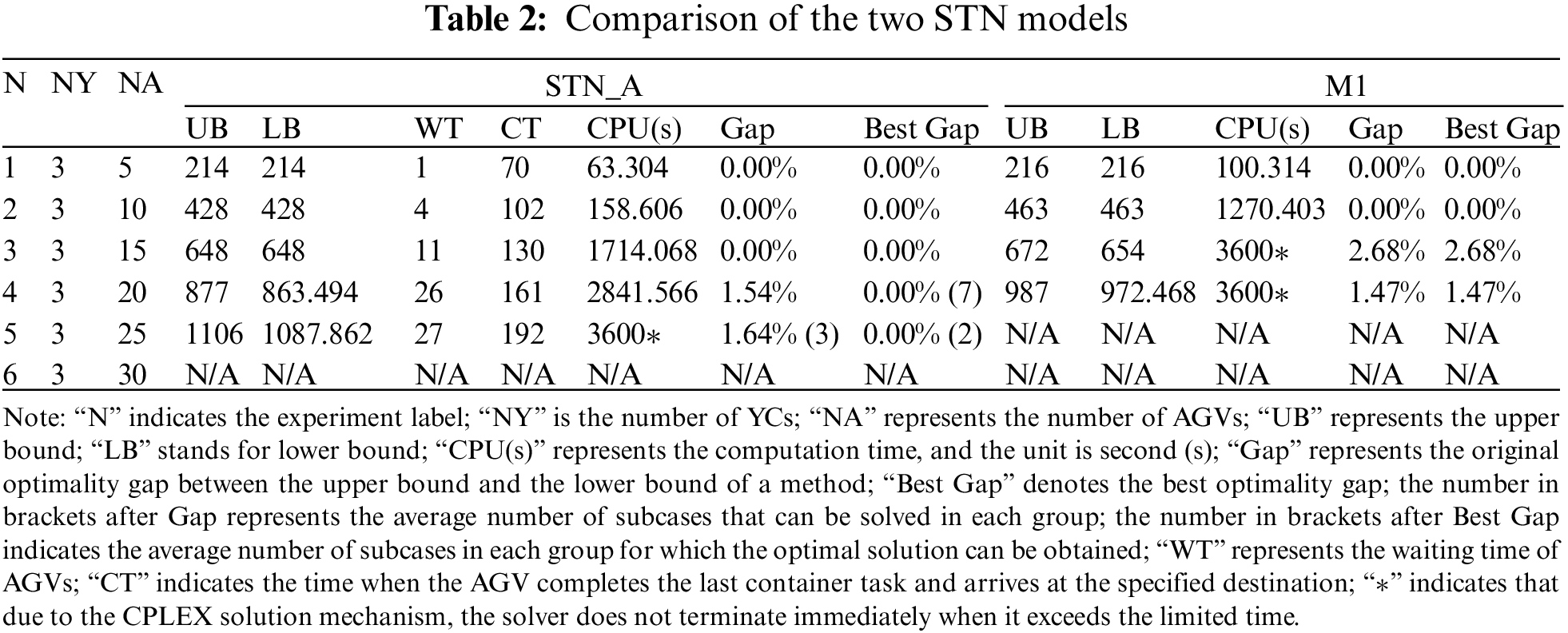
(1)   The STN_A can obtain optimal solutions of any test case in scenarios 1, 2, and 3, while M1 can only obtain optimal solutions for scenarios 1 and 2. Moreover, optimal solutions cannot be obtained by M1, while optimal solutions for 70% of all test cases in scenario 4 can be obtained by STN_A. For scenario 5, M1 fails to obtain a feasible solution, while feasible solutions for 30% of the test cases can be obtained by STN_A.

(2)   The computation times of STN_A are 49.47% shorter on average than M1 for the first four scenarios. Besides, the computation times of STN_A are 62.21% shorter than M1 on average for the first two scenarios. It can be seen that the computation times of STN_A are less than M1 for all scenarios. Moreover, the computation times of STN_A rise more slowly than those of M1 when the number of AGVs increases.

(3)   For the first four scenarios, a solution with the best gap of 0 can be obtained by STN_A and the results on the Gap of STN_A are 1.69% smaller than those of M1 on average. The maximum value in column “Gap” of STN_A is 1.04% less than the maximum value in column “Best Gap” of M1.

(4)   The above results show that a solution with the same or even better quality can be provided by STN_A than M1 in a shorter time. There are two reasons. First, the set of trajectories between different nodes has been defined separately, and the flow balance constraints in M1 have been decomposed, which can accelerate CPLEX’s search for paths. Second, constraints on the trajectories of YCs and AGVs have been added so the values of the decision variables can be determined quickly, thus speeding up the optimization process.

5.2 Comparison of Different Methods

The results of the ADMM, the heuristic rules, and CPLEX are compared. The results are shown in Tables 3 and 4 when there are 12 blocks in the yard. The results show that:

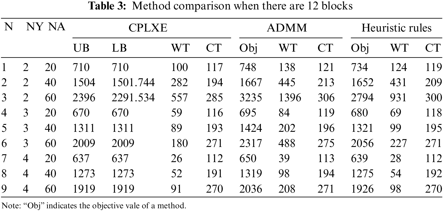
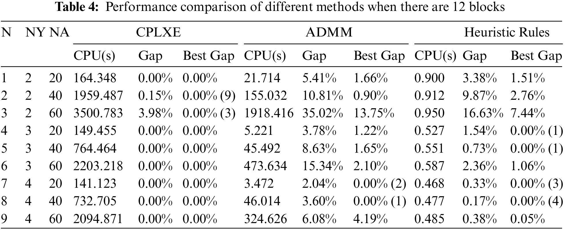
(1)   As for computation times, CPLEX takes the longest time, followed by the ADMM, and the heuristic rules take the shortest time for solving the same test case. It should be noticed that the computation time of the heuristic rules is only 0.15% of CPLEX’s on average, and it is negatively correlated with the number of YCs. Moreover, the computation time tends to increase as the number of AGVs increases when the number of YCs is fixed, but the computation time of the heuristic rules varies little. However, the computation time is negatively correlated with the number of YCs in general when the number of AGVs is fixed because the average number of tasks and the average working range of each YC can be reduced by increasing the number of YCs. Besides, the decrease in computation time decreases as the number of YCs increases when the number of AGVs is fixed, and there are two main reasons for this. One is that when the number of YCs is relatively large, a smaller T can be estimated, which leads to a smaller optimization space. The other reason is that the optimization space per YC is also smaller when the number of YCs is relatively large compared to a small number of YCs.

(2)   The probabilities of optimal solutions obtained by CPLEX, ADMM, and heuristic rules are 91.11%, 3.33%, and 10.00%, respectively. The average values of the three methods on the Gap are 0.46%, 9.03%, and 3.93%, respectively. For any scenario, the results of CPLEX on the Gap are the smallest, followed by the heuristic rules, and the ADMM is the largest. The results of the three methods show that the Gap tends to increase with a decrease in the number of YCs.

(3)   When the number of AGVs is fixed, the average values on the WT and CT decline by 59.04% and 2.09%, respectively, when the number of YC increases from 2 to 3. And the average value on the WT and CT declines by 48.98% and 1.62%, respectively, when the number of YC increases from 3 to 4. It can be inferred that the queuing time of AGVs at the same YC can be effectively reduced by increasing the number of YCs, and the maximum CT of AGVs can be slightly reduced, too. However, the value on the WT and CT can be reduced by increasing the number of YCs when the number of YCs reaches a certain value, but the reduction amplitude is smaller.

(4)   It can be found that as the number of YCs decreases, the results of ADMM on the Gap increase significantly. The performance of ADMM in this paper is not as stable as that in [8]. The reason for this phenomenon is that the moving time of the YC is considered in this paper so that the trajectories of the YC can be described more accurately. But it slows down the optimization process, and the smaller the number of YCs, the slower the optimization process will be, so it ultimately leads to a larger result of ADMM on the Gap.

5.3 Comparison with and without Buffers

Results are shown in Table 5 when the buffer capacity is 2. By comparing Table 5 with Table 2, the following observations can be made:

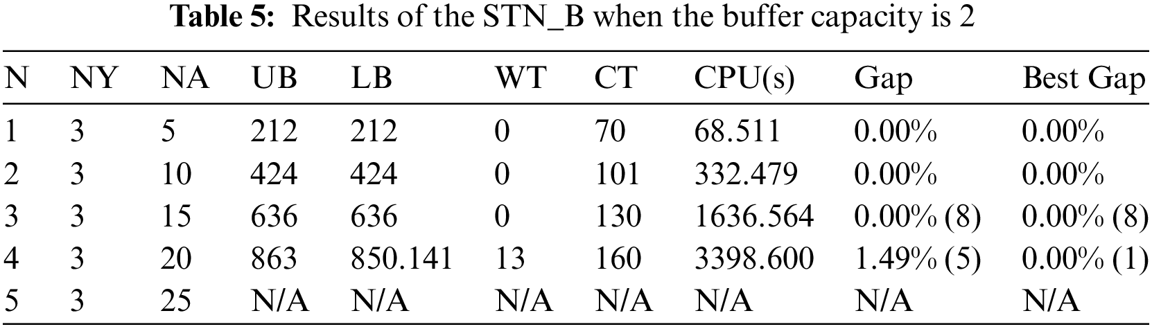
(1)   Compared with no buffers, the computation time of STN_B increases by 58.93% on average for the first two scenarios. It can be inferred that it is more difficult to solve STN_B after the buffers are added. In addition, optimal solutions can be obtained for the first two scenarios within the limited time. However, optimal or even feasible solutions cannot be guaranteed as the number of AGVs increases.

(2)   For the first three scenarios, the idle waiting time of AGVs can be significantly reduced or even eliminated after buffers are added. The UB and LB of the solution decrease after buffers are added, and their variation is basically equal to WT; that is, the decrease of UB and LB is strongly correlated with the change of WT. Regardless of the existence of buffers, the start times of the last few AGVs in the same scenario are approximately the same and the tasks are randomly generated; therefore, the CT is basically unchanged.

(3)   It can be seen that buffers do really reduce the waiting time of the AGV because the coupling relationship between YCs and AGVs is weakened after buffers are considered and the operations of YCs and AGVs become more flexible, thereby contributing to the overall operation efficiency of the ACT.

The results of the same calculation test case in scenario 4 in Tables 2 and 5 are shown in Figs. 5 and 6, respectively. They are taken as examples to illustrate the influence of buffers in the yard on the YC and the AGV. The corresponding trajectories of the YC and the AGV are represented by the red and blue lines, respectively. The labels of the AGV are represented by the numbers 1 to 20 next to the horizontal coordinate, and the departure times of AGVs are indicated by the coordinate value corresponding to the position of the number. In addition, the labels of the container tasks completed jointly by the YC and the AGV are indicated by the number marked near the overlap of their trajectories; the labels of container tasks performed by the YC and the AGV are indicated by the red and blue numbers next to the pick-up and drop-off trajectories in Fig. 6, respectively.

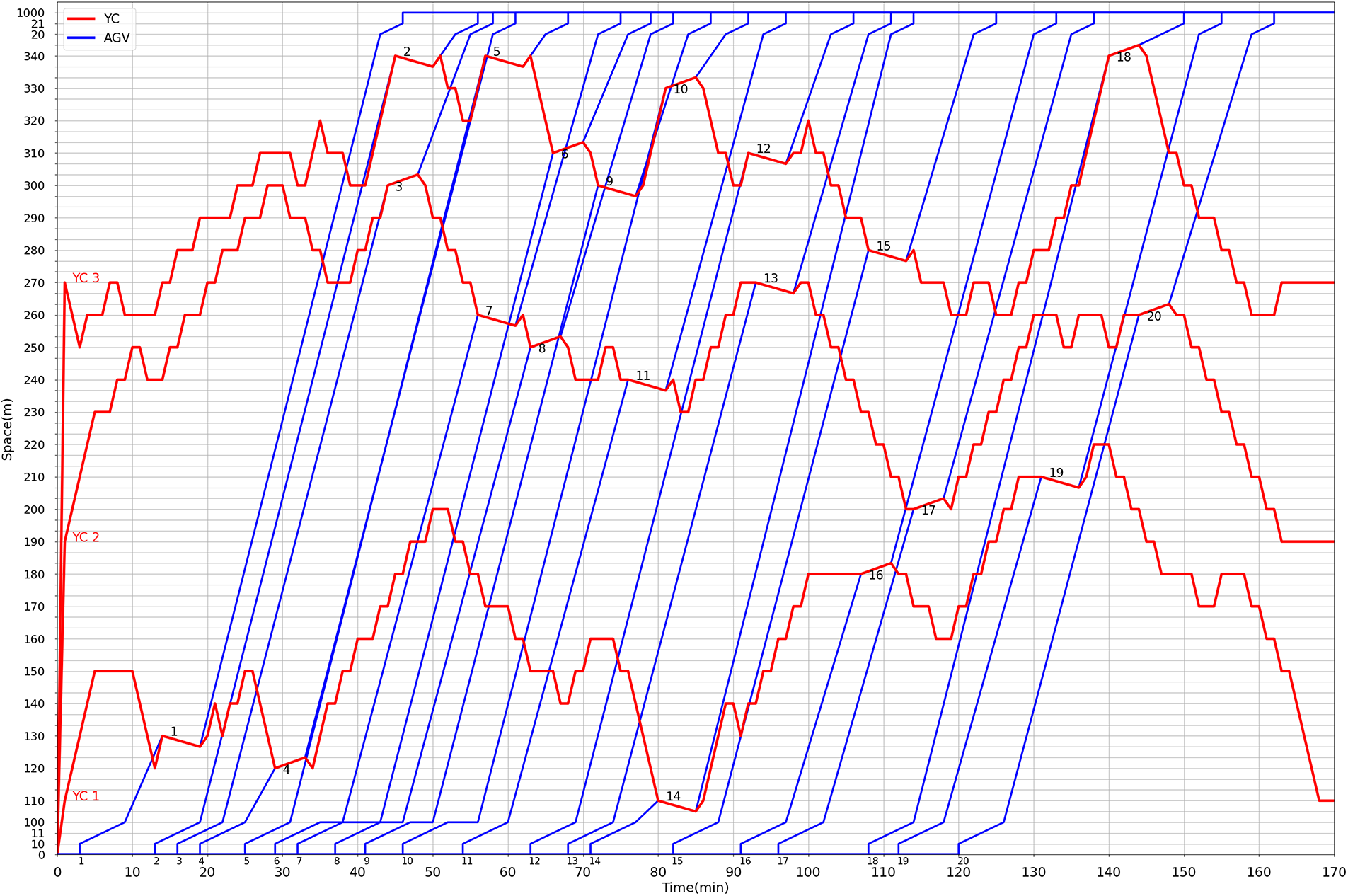
Figure 5: Results without considering buffers

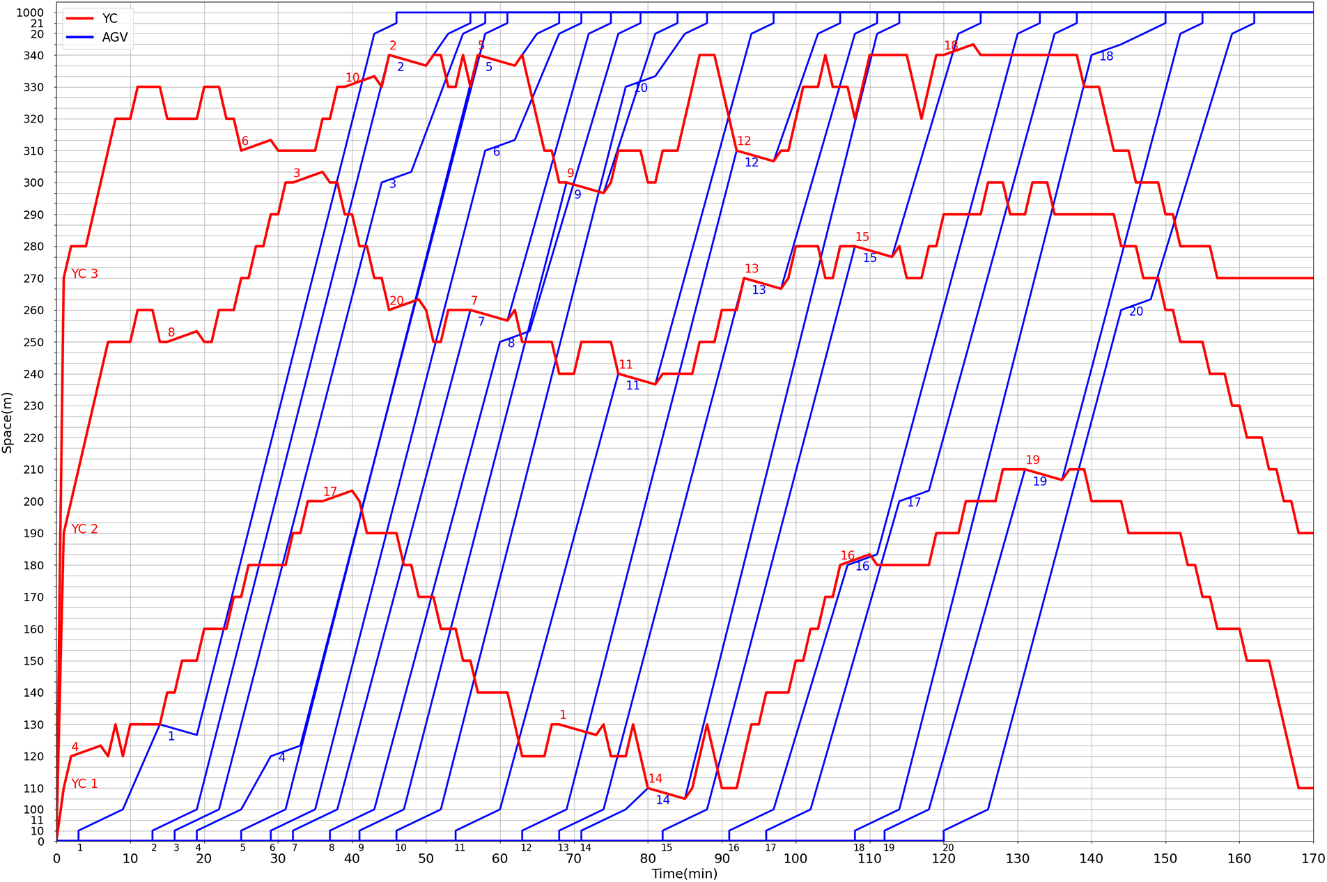
Figure 6: Results of considering buffers (buffer capacity of each block is 2)

In Fig. 5, the tasks must be completed by the YC and the AGV simultaneously at the block node when there are no buffers. Moreover, AGVs 6, 8, 9, and 10 have been waiting at the centralized waiting area node 100 in Fig. 5, while all AGVs did not wait in Fig. 6. Because container tasks can be placed in buffers by YC 3 before they are performed by AGVs 6, 8, and 10 when buffers are added. Then, the container tasks of the three AGVs can be directly performed by them when they reach the target block nodes. In addition, the main reason that causes AGV 9 to wait in Fig. 5 is that YC 3 does not cooperate with AGV 6 to complete the container task in time. However, because of the existence of buffers, the container task to be operated by AGV 6 can be placed in the buffer by YC 3 before AGV 9 reaches the target block node. Therefore, the container task can be completed cooperatively by YC 3 and AGV 9 when AGV 9 arrives at the target block node. Besides, the two buffers at node 300 are idle when AGV 9 arrives at the node to perform the drop-off task, so it will not cause AGV 9 to wait even if YC 3 does not arrive at this node in time. It can be seen from the above analysis that the coupling relationship between the YC and the AGV is weakened by the existence of the buffers, and the operations of the YC and the AGV become more flexible. Therefore, the waiting time of AGVs decreases significantly after buffers are added, and the buffers are very helpful for improving the operation efficiency of ACTs.

5.4 Comparison of Blocks with Different Numbers

Results are shown in Tables 6 and 7 when there are 24 blocks in the yard. Compared with Tables 3 and 4, it can be seen that:

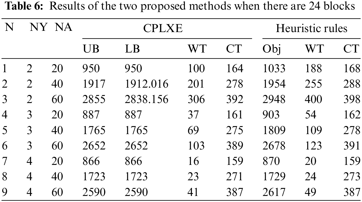
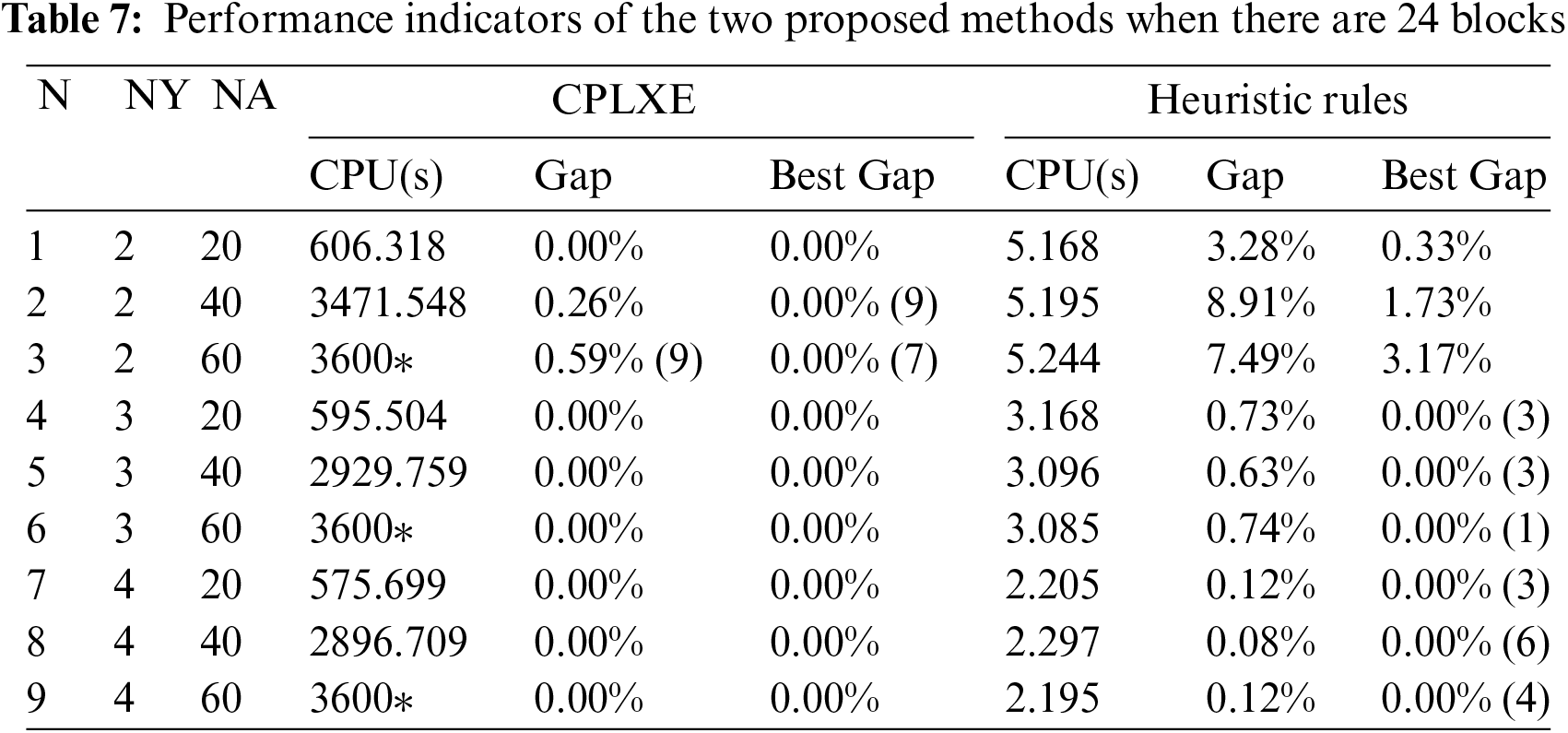
(1)   It can be seen that increasing the number of blocks increases the difficulty of CSPYA because there is an overall increasing trend in the computation times compared with the results in Table 4. The main reason is that the average working range of each YC becomes larger after increasing the number of blocks, which leads to more complex scheduling of the YC. To be more specific, the scheduling of the YC becomes more frequent and long-distance movements of the YC increase.

(2)   Optimal or near-optimal solutions can be obtained by CPLEX for most of the test cases. But as can be seen from scenario 2, the value in column “Gap” of CPLEX tends to increase. There is a test case in which a feasible solution cannot be obtained by CPLEX within the limited time for scenario 3. It means that the size of scenario 3 is close to the limit of solvable problems for CPLEX. So it can be inferred that feasible solutions to the problems cannot be obtained by CPLEX within the limited time when there are more AGVs. In addition, feasible solutions to all test cases can be obtained by heuristic rules and 22.22% of them are optimal solutions. The gap between the solution of heuristic rules and the solution of CPLEX is less than 1% when the number of YCs is greater than 2; the maximum Gap for heuristic rules is 3.28% for the case where the optimal solution for all test cases can be obtained by CPLEX.

(3)   The UB and the CT increase by 28.57% and 37.30%, respectively, on average. The reason for the increase in UB is that it takes more time for some AGVs to reach the newly added block nodes to perform their tasks, thus increasing the average distance traveled per AGV. The reason for the increase in CT of AGVs is that the time requires for the last several AGVs to reach their target block nodes increases. However, the WT of AGVs decreases with an average reduction of 32.55%, and there are two reasons. The first is due to more time spent on roads for AGVs to arrive at some block nodes to perform tasks, so the time spent by AGVs in the centralized waiting area node is reduced. The second is that the probability of arriving at the same block nodes decreases for the same number of AGVs, thus reducing the queuing times of AGVs.

6  Conclusions

In order to improve the solution efficiency of the existing STN model M1 for the CSPYA and extend its application scope, two improved STN models are proposed. The STN_A is obtained based on M1: flow balance constraints in M1 are decomposed according to the set of trajectories among different nodes; trajectory constraints are added based on the operation mode of the YC and container tasks of the AGV. Then, the STN_B is obtained based on STN_A: the flow coupling constraint in STN_A is replaced; constraints on the buffer capacity and the cooperation between YCs and AGVs are added. In order to obtain an approximate optimal solution to the problem within a short time, a heuristic method containing three groups of heuristic rules is designed. The experimental results show that compared with M1, the computation times to obtain optimal and feasible solutions of STN_A are reduced by 62.21% and 49.47% on average, respectively. For scenarios where all optimal solutions are obtained by CPLEX, solutions with comparable quality can be provided by the heuristic rules in a much shorter time. Besides, solutions to the CSPYA can be provided by solving STN_B after buffers are added, but it becomes more difficult to solve the problem. Moreover, the waiting time of AGVs is reduced after adding buffers or blocks, and the minimum of the maximum completion time of AGVs increases after increasing the number of blocks.

In this study, only the situation of fixed buffer capacity is considered. Since the demand for buffer capacity is different for different blocks at different time periods, dynamic allocation of buffer capacity can make more effective use of space resources in ACTs. Therefore, the situation of dynamic buffer capacity will be considered. In addition, the global search capability and the stability of the heuristic rules need to be improved, and intelligent optimization algorithms will be combined with them. Besides, one waiting area is shared by all AGVs in this study. The flexibility of AGVs will be further improved if there are multiple centralized waiting areas, so the cooperative scheduling problem with multiple waiting areas will be studied.

Acknowledgement: All the study was completed by the authors and there were no other contributors.

Funding Statement: This work was partly supported by National Natural Science Foundation of China (62073212).

Author Contributions: Study conception and design: Hongyan Xia, Jin Zhu; data collection: Hongyan Xia; analysis and interpretation of results: Hongyan Xia; draft manuscript preparation: Hongyan Xia; manuscript revision: Hongyan Xia, Jin Zhu.

Availability of Data and Materials: The authors confirm that the data supporting the findings of this study are available within the article.

Conflicts of Interest: The authors declare that they have no conflicts of interest to report regarding the present study.

References

1. UNCTAD (2022). Review of maritime transport 2022. https://unctad.org/system/files/official-documenty/rmt2022_en.pdf [Google Scholar]

2. Hu, Z. H., Sheu, J. B., Luo, J. X. (2016). Sequencing twin automated stacking cranes in a block at automated container terminal. Transportation Research Part C: Emerging Technologies, 69(3), 208–227. https://doi.org/10.1016/j.trc.2016.06.004 [Google Scholar] [CrossRef]

3. Meersmans, P. J. M., Wagelmans, A. P. M. (2001). Effective algorithms for integrated scheduling of handling equipment at automated container terminals. https://www.semanticscholar.org/paper/Effective-algorithms-for-integrated-scheduling-of-Meersmans-Wagelmans/1386dcf3829bd08472e74eddf3ae546091a4cdc8 [Google Scholar]

4. Jiang, X. J., Jin, J. G. (2017). A branch-and-price method for integrated yard crane deployment and container allocation in transshipment yards. Transportation Research Part B: Methodological, 98(3), 62–75. https://doi.org/10.1016/j.trb.2016.12.014 [Google Scholar] [CrossRef]

5. Zhang, Q. L., Hu, W. X., Duan, J. G., Qin, J. Y. (2021). Cooperative scheduling of AGV and ASC in automation container terminal relay operation mode. Mathematical Problems in Engineering, 2021, 1–18. https://doi.org/10.1155/2021/5764012 [Google Scholar] [CrossRef]

6. Wen, J. X., Wei, C., Yin, Y. Q., Hu, Z. H. (2020). Integrated scheduling of ASC and AGV considering block buffer capacity. Computer Engineering and Applications, 56(11), 238–245. https://doi.org/10.3778/j.issn.1002-8331.1903-0019 [Google Scholar] [CrossRef]

7. Ai, L. H., Han, X. L. (2018). Coordinated scheduling of handling equipments at automated terminals considering energy consumption. Journal of Shanghai Maritime University, 39(4), 26–31. https://doi.org/10.13340/j.jsmu.2018.04.005 [Google Scholar] [CrossRef]

8. Lu, Y. Q., Le, M. (2014). The integrated optimization of container terminal scheduling with uncertain factors. Computers & Industrial Engineering, 75(1), 209–216. https://doi.org/10.1016/j.cie.2014.06.018 [Google Scholar] [CrossRef]

9. Cheng, C. C., Liang, C. J., Li, Y. (2019). Study on AGV scheduling with considering AGV partner in automated container ports. Application Research of Computers, 36(8), 2349–2354. https://doi.org/10.19734/j.issn.1001-3695.2018.02.0091 [Google Scholar] [CrossRef]

10. Homayouni, S. M., Tang, S. H. (2016). Optimization of integrated scheduling of handling and storage operations at automated container terminals. WMU Journal of Maritime Affairs, 15(1), 17–39. https://doi.org/10.1007/s13437-015-0089-x [Google Scholar] [CrossRef]

11. Legato, P., Mazza, R. M., Trunfio, R. (2010). Simulation-based optimization for discharge/loading operations at a maritime container terminal. OR Spectrum, 32(3), 543–567. https://doi.org/10.1007/s00291-010-0207-2 [Google Scholar] [CrossRef]

12. Homayouni, S. M., Tang, S. H., Motlagh, O. (2014). A genetic algorithm for optimization of integrated scheduling of cranes, vehicles, and storage platforms at automated container terminals. Journal of Computational and Applied Mathematics, 270, 545–556. https://doi.org/10.1016/j.cam.2013.11.021 [Google Scholar] [CrossRef]

13. Lau, H. Y. K., Zhao, Y. (2008). Integrated scheduling of handling equipment at automated container terminals. International Journal of Production Economics, 112(2), 665–682. https://doi.org/10.1016/j.ijpe.2007.05.015 [Google Scholar] [CrossRef]

14. Yin, Y. Q., Zhong, M. S., Wen, X., Ge, Y. E. (2023). Scheduling quay cranes and shuttle vehicles simultaneously with limited apron buffer capacity. Computers and Operations Research, 151(1–2), 106096. https://doi.org/10.1016/j.cor.2022.106096 [Google Scholar] [CrossRef]

15. Luo, J. B., Wu, Y. (2020). Scheduling of container-handling equipment during the loading process at an automated container terminal. Computers & Industrial Engineering, 149(3), 1–12. https://doi.org/10.1016/j.cie.2020.106848 [Google Scholar] [CrossRef]

16. Lu, Y. Q. (2021). The three-stage integrated optimization of automated container terminal scheduling based on improved genetic algorithm. Mathematical Problems in Engineering, 2021(2), 1–9. https://doi.org/10.1155/2021/6792137 [Google Scholar] [CrossRef]

17. Xue, H. R., Han, X. L. (2023). Integrated scheduling considering automated guided vehicle charging strategy based on improved NSGA-II. Journal of Computer Applications. https://doi.org/10.11772/j.issn.1001-90812022121923 [Google Scholar] [CrossRef]

18. Yu, A. L., Zhang, H. Y., Chen, Q. X., Mao, N., Xi, S. H. (2021). Buffer allocation in a flow shop with capacitated batch transports. Journal of the Operational Research Society, 73(4), 888–904. https://doi.org/10.1080/01605682.2020.1866957 [Google Scholar] [CrossRef]

19. Qin, T. B., Du, Y. Q., Chen, J. H., Sha, M. (2020). Combining mixed integer programming and constraint programming to solve the integrated scheduling problem of container handling operations of a single vessel. European Journal of Operational Research, 285(3), 884–901. https://doi.org/10.1016/j.ejor.2020.02.021 [Google Scholar] [CrossRef]

20. Chen, X. C., He, S. W., Zhang, Y. X., Tong, L., Shang, P. et al. (2020). Yard crane and AGV scheduling in automated container terminal: A multi-robot task allocation framework. Transportation Research Part C: Emerging Technologies, 114(3), 241–271. https://doi.org/10.1016/j.trc.2020.02.012 [Google Scholar] [CrossRef]

21. Huang, Y. F., Hu, Z. H., Wang, Y. Z. (2021). Integrated scheduling of quay crane, AGV and yard crane with block buffer capacity considered. Journal of Dalian University of Technology, 61(3), 306–315. https://doi.org/10.7511/dllgxb202103011 [Google Scholar] [CrossRef]

22. Chen, J. H., Zhou, J. J., Zheng, Y. T., Ma, R. Z. (2022). Optimal scheduling model based on unmanned collector truck arrival time variation field bridge under balanced strategy. 5th International Conference on Advanced Algorithms and Control Engineering, Sanya, China. https://doi.org/10.1088/1742-6596/2258/1/012043 [Google Scholar] [CrossRef]

23. Zheng, H. X., Duan, S., Sun, C. (2021). Integrated optimization of yard crane scheduling and number of external container trucks considering relocation. Operations Research and Management Science, 30(9), 48–55. https://doi.org/10.12005/orms.2021.0279 [Google Scholar] [CrossRef]

24. Yang, Y. S., Zhong, M. S., Dessouky, Y., Postolache, O. (2018). An integrated scheduling method for AGV routing in automated container terminals. Computers & Industrial Engineering, 126(5), 482–493. https://doi.org/10.1016/j.cie.2018.10.007 [Google Scholar] [CrossRef]

25. Li, J. J., Yang, J. Y., Xu, B. W., Yang, Y. S., Wen, F. R. et al. (2021). Hybrid scheduling for multi-equipment at U-shape trafficked automated terminal based on chaos particle swarm optimization. Journal of Marine Science and Engineering, 9(10), 1080. https://doi.org/10.3390/jmse9101080 [Google Scholar] [CrossRef]

26. Li, J. J., Yan, L. X., Xu, B. W. (2023). Research on multi-equipment cluster scheduling of U-shaped automated terminal yard and railway yard. Journal of Marine Science and Engineering, 11(2), 417. https://doi.org/10.3390/jmse11020417 [Google Scholar] [CrossRef]

27. Chu, L. Y., Zhou, Y. P., Yao, Y. F., Xu, X. W. (2022). Co-scheduling optimization of multiple resources in the automated terminal considering AGV path conflict. Journal of Harbin Engineering University, 43(10), 1539–1546. https://doi.org/10.11990/jheu.202105063 [Google Scholar] [CrossRef]

28. Xin, J. B., Negenborn, R. R., Corman, F., Lodewijks, G. (2015). Control of interacting machines in automated container terminals using a sequential planning approach for collision avoidance. Transportation Research Part C: Emerging Technologies, 60, 377–396. https://doi.org/10.1016/j.trc.2015.09.002 [Google Scholar] [CrossRef]

29. Zhong, Z. L., Kong, S., Zhang, J. H., Guo, Y. Y. (2022). Integrated optimization of container terminal equipment configuration and scheduling. Computer Engineering and Applications, 58(10), 263–275. https://doi.org/10.3778/j.issn.1002-8331.2104-0337 [Google Scholar] [CrossRef]

30. Chang, Y. M., Zhu, X. N., Yan, B. C., Wang, L. (2017). Integrated scheduling of handling operations in container terminal under rail-water intermodal transportation. Journal of Transportation Systems Engineering and Information Technology, 17(4), 40–47. https://doi.org/10.16097/j.cnki.1009-6744.2017.04.007 [Google Scholar] [CrossRef]

31. He, J. L., Huang, Y. F., Yan, W. (2015). Yard crane scheduling in a container terminal for the trade-off between efficiency and energy consumption. Advanced Engineering Informatics, 29(1), 59–75. https://doi.org/10.1016/j.aei.2014.09.003 [Google Scholar] [CrossRef]

32. Zhong, M. S., Yang, Y. S., Zhou, Y., Postolache, O. (2020). Application of hybrid GA-PSO based on intelligent control fuzzy system in the integrated scheduling in automated container terminal. Journal of Intelligent & Fuzzy Systems, 39(2), 1525–1538. https://doi.org/10.3233/JIFS-179926 [Google Scholar] [CrossRef]

33. Yang, Y. J., Zhu, X. N., Haghani, A. (2019). Multiple equipment integrated scheduling and storage space allocation in rail-water intermodal container terminals considering energy efficiency. Transportation Research Record: Journal of the Transportation Research Board, 2673(3), 199–209. https://doi.org/10.1177/0361198118825474 [Google Scholar] [CrossRef]

34. Lu, B., Lv, J. Z., Zeng, Q. C. (2017). Integrated optimization model for automated lifting vehicles scheduling and yard allocation at automated container terminals. Systems Engineering-Theory & Practice, 37(5), 1349–1359. https://doi.org/10.12011/1000-6788(2017)05-1349-11 [Google Scholar] [CrossRef]

35. Jonker, T., Duinkerken, M. B., Yorke-Smith, N., de Wall, A., Negenborn, R. R. (2021). Coordinated optimization of equipment operations in a container terminal. Flexible Services and Manufacturing Journal, 33(2), 281–311. https://doi.org/10.1007/s10696-019-09366-3 [Google Scholar] [CrossRef]

36. Li, H., Peng, J. B., Wang, X., Wan, J. L. (2020). Integrated resource assignment and scheduling optimization with limited critical equipment constraints at an automated container terminal. IEEE Transactions on Intelligent Transportation Systems, 12(22), 7607–7618. https://doi.org/10.1109/TITS.2020.3005854 [Google Scholar] [CrossRef]

37. Wu, Y. Y., Zhu, J., Liu, B., Zheng, Y. C. (2018). Optimization for integrated scheduling of key equipments at automated terminal using modified genetic algorithm. Computer Simulation, 35(3), 381–384+421. [Google Scholar]

38. Gao, Y. L., Hu, Z. H. (2020). Path planning for automated guided vehicles based on tempo-spatial network at automated container terminal. Journal of Computer Applications, 40(7), 2155–2163. https://doi.org/10.11772/j.issn.1001-9081.2019122117 [Google Scholar] [CrossRef]

39. Wang, P. L., Liang, C. J., Wang, L. (2022). Multi-layer equipment scheduling and simulation analysis of automated container terminal. Computer Engineering and Applications. https://kns.cnki.net/kcms/detail/11.2127.TP.20221128.1913.033.html [Google Scholar]

40. Nguyen, V. D., Kim, K. H. (2009). A dispatching method for automated lifting vehicles in automated port container terminals. Computers & Industrial Engineering, 56(3), 1002–1020. https://doi.org/10.1016/j.cie.2008.09.009 [Google Scholar] [CrossRef]

41. Lan, P. Z., Chen, J. W., Cao, S. L. (2020). An AGV control algorithm in automated terminal based on ant-agent. Journal of Transportation Systems Engineering and Information Technology, 20(1), 190–197. https://doi.org/10.16097/j.cnki.1009-6744.2020.01.028 [Google Scholar] [CrossRef]

42. Chen, L., Langevin, A., Lu, Z. Q. (2013). Integrated scheduling of crane handling and truck transportation in a maritime container terminal. European Journal of Operational Research, 225(1), 142–152. https://doi.org/10.1016/j.ejor.2012.09.019 [Google Scholar] [CrossRef]

43. Yang, Y. J., Chang, D. F., Yu, F. (2020). Multi-resource coordinated scheduling of automated terminals considering AGV collision avoidance. Computer Engineering and Applications, 56(6), 246–253. https://doi.org/10.3778/j.issn.1002-8331.1812-0069 [Google Scholar] [CrossRef]