System Reliability Analysis Method Based on T-S FTA and HE-BN

1  Introduction

The system is a complex of many interacting and connected elements that are capable of performing a specific function. Quantifying the impact of system or human failure on a specific function is the content of system reliability analysis. For the reliability analysis of complex systems in military engineering, aerospace, rail transportation, and other fields, the system structure and operating environment are complex, the test costs are expensive and the historical failure data are insufficient [1,2]. So how to build a reliability model that is easy to calculate and completely reflects the failure characteristics of the system? How to overcome the lack of reliability data and effectively identify the weak points of the system? These are the main problems in the reliability analysis of complex systems. Therefore, it is necessary to propose a new reliability analysis method that can effectively solve these problems.

System reliability is studied for the system as a whole. However, the concept of a system as a whole is relative. The components that make up a whole system can be seen as subsystems of the whole system. This whole system can in turn be seen as subsystems of a larger whole system. The study of system reliability requires the selection of suitable analysis methods according to different applications, different analysis purposes, and different system characteristics. Commonly used traditional system reliability analysis methods include the Reliability block diagram (RBD) method, Fault tree analysis (FTA) method, Bayesian network, Markov analysis, GO method, and Petri net, etc. These traditional reliability analysis methods are mainly based on exact probability theory. However, the reliability information of complex systems is diverse and uncertain, and the reliability data is difficult to obtain [3,4]. So, the above traditional reliability analysis methods are not applicable anymore. Therefore, some scholars have introduced uncertainty characterization methods such as fuzzy theory [5], interval analysis [6], and probabilistic boxes [7] into reliability analysis.

The fault tree is an intuitive reliability modeling method that adequately represents component and system interactions and fault relationships. It has certain advantages for rapid modeling. When complex systems and equipment fail due to multiple causes and the causal relationship between higher and lower-level fault events is unclear, fault trees can be used to describe the links between fault events deterministically through logic gates. The system can then be analyzed qualitatively (to obtain the minimum cut set) and quantitatively (to obtain the top event reliability data and the bottom event importance). It has been widely used in the aerospace [8], transportation [9], and power [10] fields. Based on the fault tree, the Takagi-Sugeno Fault tree analysis (T-S FTA) method is further proposed to solve the problem of system fault polymorphism and uncertainty of the fault mechanism and data [11]. T-S fault tree has been applied to the reliability analysis of multi-state complex systems [12–14]. However, when used to calculate the top event probability of system fault trees in real engineering, the current T-S FTA is computationally intensive and cannot be backward calculated. BN fills exactly this gap and is widely used in reliability analysis [15,16].

BN uses conditional probabilities to describe the relationships between events in a fault tree. It has powerful inference and analysis capabilities. It is more suitable for complex systems in terms of representing polymorphic events, describing node relationships, and computational analysis capabilities. Therefore, the FTA model constructed based on the fault mechanism is transformed into BN inference to diagnose faults. It becomes a hot spot in the field of fault research of complex systems. In [17], the work focused on the use of BN to deal with the uncertainty of accidents and the limitations of the fault tree. In [18], a multistate fault tree was transformed into a BN model. The reliability of a semi-submersible drilling rig system under different fault states was calculated.

In the above study, BN requires large amounts of accurate fault data. Sample data are scarce for most high-reliability systems in practical engineering. The randomness assumption or fuzziness assumption is not satisfied, but it is easy to determine the uncertain information boundaries. Therefore, some scholars have introduced methods such as Fuzzy theory, Interval analysis, and Evidence theory into traditional Bayesian networks. To propose the interval Bayesian network, interval probabilities are used instead of exact probabilities. It is used to solve the problem of the influence of uncertainty and incomplete information on the reliability assessment results. The interval triangular fuzzy number is used to describe Bayesian network node probabilities for the analysis of cognitive uncertainty and failure correlation in complex multistate systems [19]. The fuzzy prior probability interval of BN is obtained by fusing highly conflicting data through D-S evidence theory to perform risk assessment [20]. In [21], the interval probability was used to quantify the cognitive uncertainty of BN, and the Bayesian posterior interval probabilities were solved using the GL2U (Generalised Loopy 2-Updating) algorithm. The interval Bayesian network calculates the upper-level node failure interval when each root node failure interval is simultaneously taking an interval extreme value. This simultaneous taking of extremes is difficult to achieve in practical engineering. For the interval Bayesian network, only upper and lower bounds on the probability of node intervals are used for system reliability analysis. The correlation of the number of intervals is not taken into account. The results of the calculations are coarse and conservative.

The Hyper-ellipsoidal model is a convex set model. The analytical description of uncertain interval covariate correlations using the HM can effectively circumvent the extreme cases of interval Bayesian models [22–24]. Therefore, the Hyper-ellipsoidal model has been applied to fatigue life analysis [25] and structural reliability analysis [26]. The introduction of convex models into the T-S FTA method to define uncertain covariate boundaries or ranges [27]. Then the problem of relatively conservative interval T-S FTA results can be solved. The HM was used to describe the uncertain interval variables of the system fault tree model for reliability assessment, which is more in line with engineeringpractice [28,29].

Based on the above considerations, this paper proposes a system reliability analysis method based on T-S FTA and HE-BN. The main contributions of this paper are as follows:

1.    A reliability modeling method that reflects complex system failure characteristics is proposed. It improves modeling and computational efficiency over traditional reliability analysis methods.

2.    The method can effectively deal with the problem of insufficient system failure data and uncertainty about the degree of failure.

3.    The method solves the problem of relatively conservative calculation results when the traditional interval Bayesian network describes uncertainty fault data. It is more in line with engineering practice.

The rest of the paper is organized as follows: In Section 2, the mapping relationship between T-S FTA and BN in terms of structure and working principle is analyzed. The D-S evidence theory and the HM are briefly reviewed. In Section 3, a reliability analysis method based on T-S FTA and HE-BN is proposed. Section 4 presents a case study on the reliability analysis of complex systems. The validity of the proposed method is illustrated. Finally, Section 5 presents the concluding remarks.

2  Introduction of Basic Theory

2.1 T-S Fault Tree and Bayesian Network

The T-S FTA is an analysis method that considers the impact of multiple fault levels on the system. It has IF-THEN rules and describes inter-event connections with T-S gates. When the input event fault state of the IF-THEN rule is two-state and the output event satisfies the traditional fault tree logic gates, the T-S Fault tree degenerates to the traditional fault tree. The traditional fault tree is a special case of the T-S Fault tree. The T-S Fault tree model is shown in Fig. 1a, where X1, X2, and X3 are bottom events, M1 is the middle event, M2 is the top event, and T-S gate 1 and T-S gate 2 are T-S fuzzy gates.

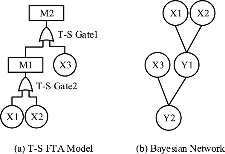
Figure 1: Model comparison

Considering the fuzziness of the event fault state, the T-S FTA uses the fuzzy number to describe the event fault state. For example, the fault state of the T-S gate input event xi(i=1,2,…,n) is a fuzzy number xi[ai](ai=1,2,…,ki). The fault state of the output event y is a fuzzy number y[bj](bj=1,2,…,nj). Then the fault logic relationship between the events can be described by the T-S gate rules. Rule l(l=1,2,…,r): If the input event x1 fault state is x1[a1], input event x2 fault state is x2[a2],… , and input event xn fault state is xn[an], the probability of output event fault state y[bj] is Pl(y[bj]). Among them, r is the total number of T-S rules that satisfy r=k1k2…kn=∏i=1n⁡ki.

The Bayesian network is a directed acyclic network composed of a directed acyclic graph and a conditional probability table, as shown in Fig. 1b. Where X1, X2, and X3 are the root nodes, Y1 is the intermediate node, and Y2 is the leaf node. X1, X2, and X3 are the parent nodes of Y1, and Y2 is the child node of Y1. The nodes are connected by directed edges and the strength of the connection is determined by the conditional probability P. P consists of conditional probability parameters between variables. The probability distribution P(X) of the BN in Fig. 1b is:

P(X)=P(X1,X2,X3)=∏i=13⁡P(Xi|Pa(Xi))(1)

where Pa(Xi) is the parent node set of nodes Xi. When Pa(Xi) is an empty set, P(Xi|Pa(Xi)) is the prior probability P(Xi) of node Xi.

The T-S FTA solves the problem of uncertainty about the failure mechanism and the degree of failure in complex systems. However, it is computationally complex and cannot be reasoned backward. And BN is superior to T-S FTA in computational analysis [17]. However, it is more difficult to construct BN directly.

2.2 D-S Evidence Theory

The fault tree analysis method based on the fuzzy reliability model is relatively mature. However, in engineering practice, it is often difficult to obtain sufficient data to determine the probability density function or fuzzy affiliation function of parameters [30]. As a mathematical method to deal with uncertainty inference problems, D-S evidence theory quantifies the degree of confidence and likelihood of propositions. It captures the unknown and uncertainty of the problem better than the traditional probability theory. It provides a way to obtain input data in fault tree analysis.

D-S evidence theory is a theory of information fusion [31]. It expresses the uncertainty problem through the belief function and the plausibility function [32]. Define the discernment framework Θ, which consists of several completely mutually incompatible elements. Denote A as any subset of the discernment framework Θ. Define the basic creditability allocation function for the evidence i to be mi:2Θ→[0,1] (2Θ is a powerful set of Θ) satisfying:

{m(∅)=0∑A⊆Θ⁡m(A)=1(2)

Define the belief degree Bel: 2Θ→[0,1] and plausibility degree Pl: 2Θ→[0,1]. When ∀A⊆Θ, and A≠∅, there are Bel(A)=∑B⊆A⁡m(B), Pl(A)=∑B∩A≠∅⁡m(B), Bel(A)=1−Pl(A).

According to the D-S synthesis rule, the synthesis rule for n pieces of independent evidence on the identification frame Θ as shown in Eq. (3):

m(A)=(m1⊕m2⊕⋯⊕mn)(Ai)=1K∑A1∩A1∩⋯∩An=A⁡∏j=1n⁡mj(Ai)(3)

Among them, K is the normalization factor, which is used to measure the degree of conflict between evidence, and can be obtained by Eq. (4):

K=∑A1∩A1∩⋯∩An≠∅∏j=1n⁡mj(Ai)=1−∑A1∩A1∩⋯∩An=∅⁡∏j=1n⁡mj(Ai)(4)

2.3 Hyper-Ellipsoidal Model

The D-S theory of evidence cannot resolve serious conflicts and complete conflicts in the evidence. And the more the number of elements in a subset, the greater the ambiguity of the subset. HM is a convex set model. It has the advantages of continuous parameter variation, simple model structure, and easy correlation analysis. It can better compensate for the lack of too-conservative analysis results of the Interval model [22], as shown in Fig. 2.

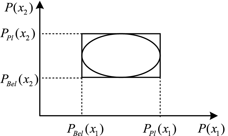
Figure 2: Two-dimensional interval model and two-dimensional hyper-ellipsoidal model

The HM is a method of reflecting the deviation of a random variable based on the distance between its equivalent unit hypersphere coordinate origin and the failure surface of a structure in normalized vector space. If the random variable Xi∈[xiL,xiU](i=1,2,⋯,n) in the set of random variables X, where xiL and xiU are the lower bound and upper bound of the value of Xi, respectively. Then the HM of the set of random variables X is described as:

[X1−x10x1,⋯,Xn−xn0xnr]T⋅[X1−x10x1,⋯,Xn−xn0xnr]≤1(5)

where, xi0=xiL+xiU2, xir=−xiL+xiU2 are the nominal value and the deviation of xi, respectively.

3  T-S FTA and HE-BN Reliability Analysis Methods of Coupler System

Conditional probability tables for BN are difficult to construct. The T-S FTA method is computationally complex and cannot be reasoned backward. Using the Interval model to describe the failure probability of the root node is relatively conservative. To address these problems, a reliability analysis method based on T-S FTA and HE-BN is proposed. Firstly, a T-S fuzzy gate is used to describe the connection between each failure event of the system. Then the BN model of the system is constructed. Secondly, experts describe the event failure degree in the form of interval numbers. The knowledge and experience of several experts are fused using the D-S evidence theory. The initial failure probability interval of each root node of the BN is obtained. Then the Hyper-ellipsoidal Model (HM) constrains the initial failure probability interval. The HE-BN model of the system is constructed. Finally, the probability of failure of the system is inferred and calculated to find out the key components of the system. The analysis process is shown in Fig. 3, and the analysis steps are as follows:

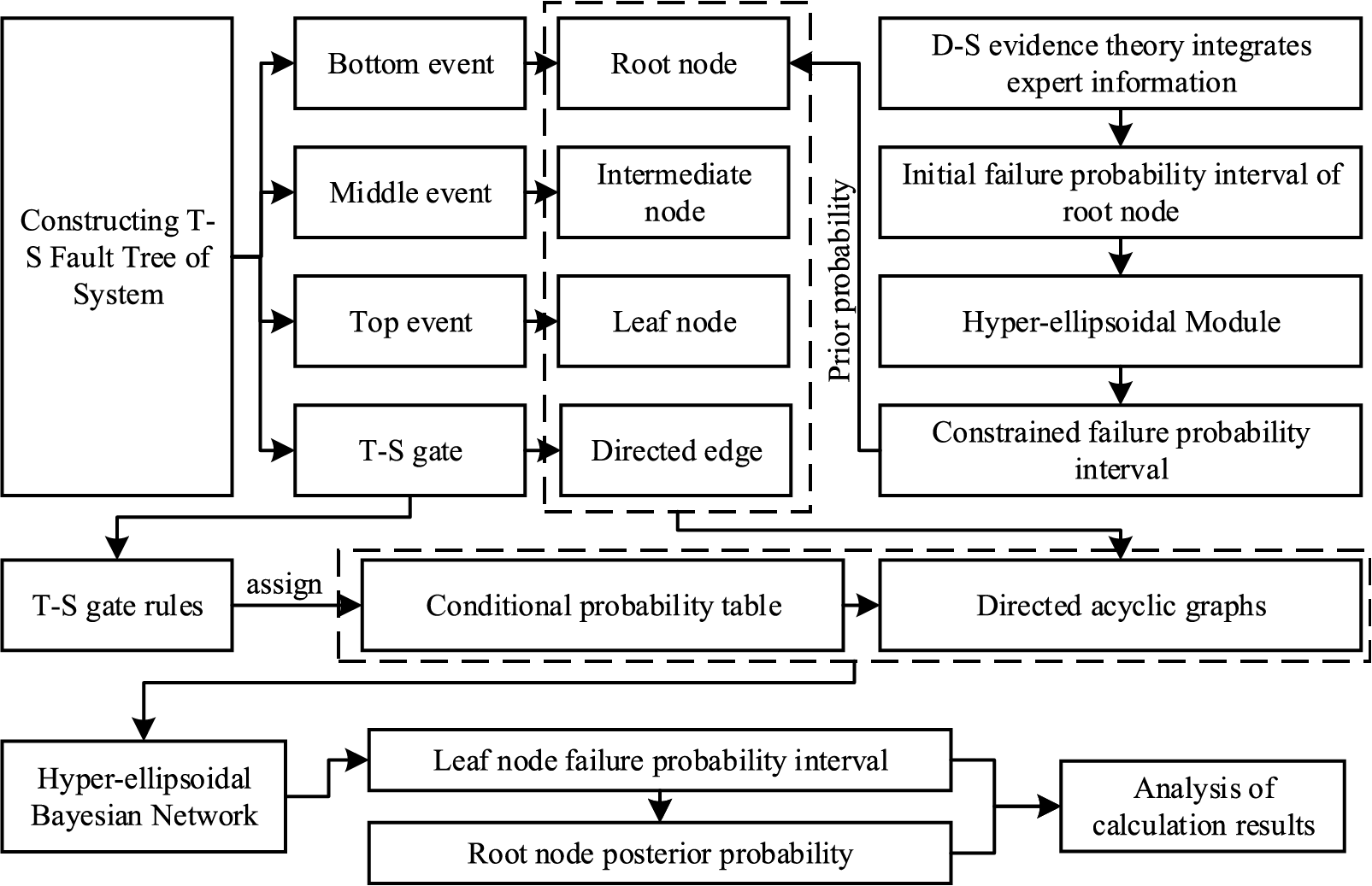
Figure 3: T-S FTA and HE-BN reliability analysis process

Step 1: Analyse the system structure and working principle. Determine the top event T and the bottom event Xi(i=1,2,3,⋯,n). Connect them with a T-S gate to construct a T-S fault tree model of the system. Describe the fuzzy fault occurrence probability of the bottom event by the interval number P(Xi)=[xiL,xiU](i=1,2,⋯,n). T-S gate rule l is expressed as P(l)(y[n]).

Step 2: Transform the T-S FTA into a BN model according to Fig. 3.

In the working principle, the T-S FTA and BN can be mapped from one to another. Each event in the T-S FTA corresponds to a BN node. The T-S gate rule and the conditional probability table of the BN can also be mapped, see Table 1. Therefore, the T-S FTA can be used as a reference to build a BN quickly and efficiently.

The events in the T-S fault tree are transformed into nodes one by one according to the correspondence in Fig. 3 and Table 1. The state of each event corresponds to the state of each node. The nodes are connected using directed edges according to the logic of T-S gates. The probability of failure P(Xi)=[xiL,xiU](i=1,2,⋯,n) of the bottom event is assigned to the root node as the prior probability. The T-S gate rules are described using the conditional probability table P(y=y[n]|x1=x1[a1],⋯,xn=xn[an]).

Step 3: A component or system will go through multiple states from a normal operating state to a complete fault state in actual engineering. This paper assumes that the Bayesian network model component or system has three states. The fault state of the system node in the BN is defined as fault occurrence, fault non-occurrence, and fault in a fuzzy uncertainty state. Then the system discernment framework is Θ= {Fault occurrence, Fault non-occurrence, Fault in fuzzy uncertainty state}, denoted as Θ = {A1, A2, (A1,A2)}, see Table 2. There are also two states of nodes in the BN. The fault state of the node is defined as fault occurrence, fault non-occurrence, then the discernment framework is Θ = {Fault occurrence, Fault non-occurrence}, denoted as Θ = {A1, A2 }. It is calculated in the same way as the three-state node.

Step 4: Adopt expert knowledge and experience as the body of evidence. The two experts make their judgments about the probability of the state of the various root nodes. Denote their judgments as evidence Z1, Z2. Construct the basic credibility distribution function for the root node, see Table 2.

Step 5: According to the D-S synthesis rule, the root node Xi failure probability interval was calculated under the joint action of two experts’ evidence. Calculating the conflict value according to Eq. (6), and the synthesis results are shown in Table 3.

k=∑Ai∩Aj=∅⁡s1(Ai)s2(Aj)=m1(1−m2−n2)+m2(1−m1−n1)(6)

The failure probability interval of the root node Xi is shown in Eq. (7).

P(Xi)=[Bel,Pl]=[m1m2+m1n2+m2n11−k,(m1+n1)(m2+n2)1−k](7)

Step 6: Constrain the root node initial failure probability interval using the HM to obtain the root node probability interval P(Xi) in BN analysis.

In BN, the greater the number of BN nodes, the less likely it is that their failure intervals will require simultaneous bounds. This simultaneous taking of bounds is thus negligible in the reliability analysis of complex systems [22]. Therefore, a Hyper-ellipsoidal domain can be used to deal with Bayesian network node intervals. That is, the uniformly distributed points satisfying Eq. (5) are extracted within the interval box model. The failure probability interval of each root node of the BN is obtained.

And for multidimensional variables, to enhance the efficiency of sampling, sampling can be carried out according to Eqs. (8)–(12).

Introduce vector:

z=D−1P(8)

{z=(z1,z2,…,zn)TD=diag(Pr(X1),Pr(X2),…,Pr(Xn))P=[P(X1),P(X2),…,P(Xn)]T(9)

Eq. (5) is converted into:

(z−z0)T⋅(z−z0)≤1(10)

z0=[P0(X1)Pr(X1),P0(X2)Pr(X2),⋯,P0(Xn)Pr(Xn)]T(11)

From Eq. (10), generating uniformly distributed random numbers in the hyper-ellipsoid is equivalent to uniform sampling in the unit hypersphere of Δz space. The interval probability of the root node shall be uniformly taken within the space hyper-ellipsoid Δz=z−z0. Let the unit hyper-ellipsoidal coordinate be (r,θ1,θ2,⋯,θn−1), where r∈[0,1], θi∈[0,2π] , then:

Δz=z−z0=[rcos⁡θ1rsin⁡θ1cos⁡θ2⋮rsin⁡θ1sin⁡θ2⋯sin⁡θn−3cos⁡θn−2rsin⁡θ1sin⁡θ2⋯sin⁡θn−2cos⁡θn−1](12)

The HM of interval probability P(Xi) of the root node Xi of BN is:

[P(Xi)−P0(Xi)Pr(Xi),⋯,P(Xn)−P0(Xn)Pr(Xn)]T⋅[P(Xi)−P0(Xi)Pr(Xi),⋯,P(Xn)−P0(Xn)Pr(Xn)]≤1(13)

where P0(Xi)=Bel(Xi)+Pl(Xi)2 is the nominal value of P(Xi); Pr(Xi)=−Bel(Xi)+Pl(Xi)2 is the deviation of P(Xi).

According to Eqs. (8)–(12), the interval probability P(Xi) of the root node is:

{P(X1)=Pr(X1)rcos⁡θ1+P0(X1)P(X2)=Pr(X2)rsin⁡θ1cos⁡θ2+P0(X2)⋮P(Xn−1)=Pr(Xn−1)rsin⁡θ1…sin⁡θn−2sin⁡θn−1+P0(Xn−1)P(Xn)=Pr(Xn)rsin⁡θ1…sin⁡θn−2sin⁡θn−1+P0(Xn)(14)

Step 7: The HE-BN is used for forward calculation, and the failure probability interval of the leaf node T with fault state Tq is obtained as shown in (15).

P(T=Tq)=∑x1,x2,…,xn;y1,y2,…,ymP(x1,x2,…,xn;y1,y2,…,ym;T=Tq)=∑λ(T)⁡P(T=Tq|λ(T))×∑λ(y1)⁡P(y1|λ(y1))∑λ(y2)⁡P(y2|λ(y1))×⋯×∑λ(ym)P(ym|λ(ym))P(x1a1)P(x2a2)⋯P(xnan)(15)

where P(xiai) is the interval probability of fault occurs when the fault state of the root node xi is xiai.

Step 8: When the fault state of the leaf node is known to be Tq, the posterior probability P(xi=xiai|T=Tq) of the root node xi with fault state xiai is obtained as Eq. (16).

P(xi=xiai|T=Tq)=P(xi=xiai,T=Tq)P(T=Tq)=∑x1,x2,…,xn⁡P(x1,…,xi=xiai…xn,T=Tq)P(T=Tq)  =P(xiai)P(T=Tq)∑x1,x2,…,xn⁡P(T=Tq|x1,…,xi=xiai…xn)⋅P(xia1)…P(xi−1ai−1)P(xi+1ai+1)…P(xnan)(16)

where P(xi=xiai,T=Tq) is the joint probability of the root node xi with the fault state xiai and the leaf node T with the fault state Tq.

4  Application Case Analysis

4.1 Multistate Series-Parallel Systems Reliability Analysis

The multistate series-parallel system is shown in Fig. 4. Construct its T-S fault tree as shown in Fig. 5a, where G1 denotes “AND” gates. G2 and G3 denote “OR” gates. The Fault occurrence state, Fault in fuzzy uncertainty state, and Fault non-occurrence state of the system and components are denoted by A1,(A1,A2), and A2. The failure rate of the component Xi(i=1,2,3,4) in the Fault occurrence state is 5.0×10−5/h, 1.0×10−5/h, 1.5×10−5/h, and 1.2×10−5/h, respectively. The failure rate of components in the Fault in fuzzy uncertainty state is 9.0×10−5/h, 1.0×10−4/h, 2.8×10−5/h, and 3.6×10−5/h, respectively.

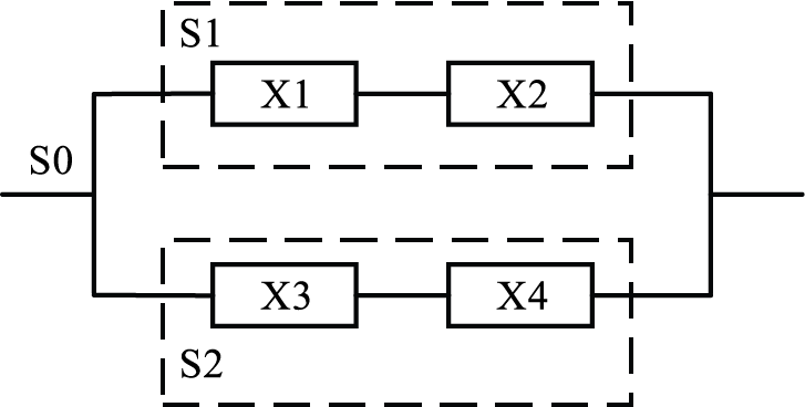
Figure 4: Multistate series-parallel systems

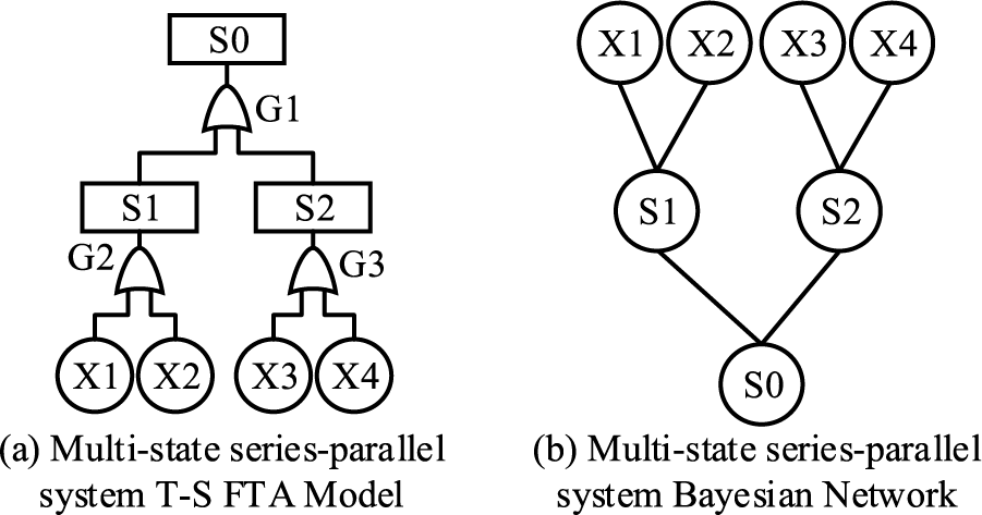
Figure 5: Reliability model for a multi-state series-parallel system

The T-S FTA of the multistate series-parallel system was converted into a BN as shown in Fig. 5b. The T-S gate rules are converted into a conditional probability table. For the G1 gate, see Table 4. Conditional probability tables are the same for G2 and G3, see Table 5. Table 4 rule 1 indicates that under the condition that the S1 state is A1, S2 state is A1, the probability of S0 state A1 is 1 and the probability of (A1,A2) and A2 is 0. Other rules can be followed in this way.

First, the multistate series-parallel system is analyzed by the traditional Bayesian network method. Based on the conditional probability table and the exact failure rate of each root node, the probability of the Fault occurrence state of the leaf node is calculated to be P(S0=A1)=298299.7969×10−14, the probability of the Fault in fuzzy uncertainty state is P(S0=(A1,A2))=738060.0823×10−14, and the probability of the Fault non-occurrence state is P(S0=A2)=999999.9963×10−6. The multistate series-parallel system was analyzed using the interval Bayesian network and the method proposed in this paper. Table 6 shows the failure rates at each root node.

Probability at each state of leaf nodes was obtained by the Bayesian inference algorithm. The comparative analysis results of the traditional Bayesian network, the interval Bayesian network, and the method proposed in this paper are shown in Table 7.

The system failure rate is assumed exponentially distributed. The reliability curves of the multistate series-parallel system under the three methods are obtained as shown in Fig. 6.

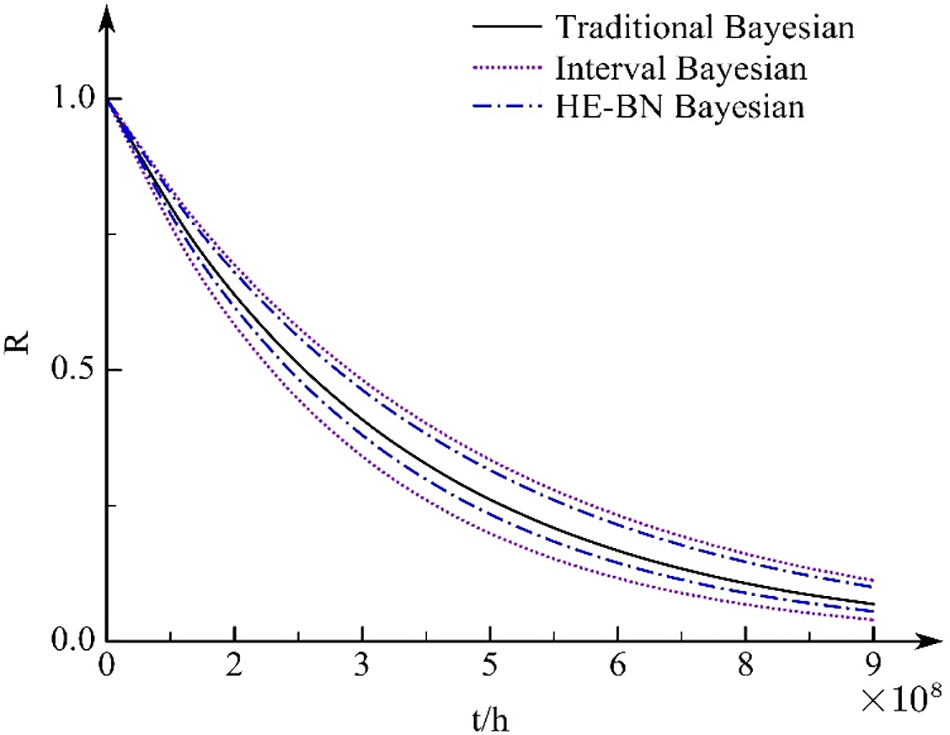
Figure 6: Multistate series-parallel system reliability curves

As can be seen from Table 7 and Fig. 6, the traditional Bayesian analysis results using exact failure rates are within the HE-BN method interval results. Also, the length of the analysis result interval for HE-BN is smaller and closer to the exact value than the interval Bayesian results. It proves that the present method can solve the problem of insufficient failure data. It can also make up for the relatively conservative calculation results of the Interval model, which is more in line with engineering practice.

Using the HE-BN method, the posterior probability of each root node is calculated by Eq. (16) when the multistate series-parallel system is in the fault occurrence state. The posterior probability results are sorted by the interval number sorting method based on the order relationship. For the interval number A[a−,a+], define the measurement mθ(a)=(1−θ)a−+θa+ of the interval numbers, θ∈[0,1]. The larger the value of mθ(a), the larger the corresponding interval number. After sorting them by the interval number sorting method [33], a comparison with traditional Bayesian results is shown in Fig. 7.

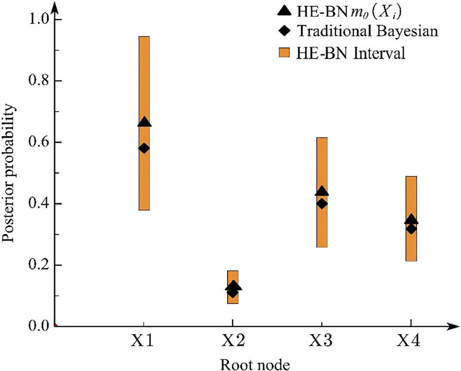
Figure 7: Comparing posterior probability results for multistate series-parallel system root nodes

As can be seen from Fig. 7, the method proposed in this paper is consistent with the results of the posterior probability ranking of the root nodes obtained from the traditional Bayesian method. The results are X1>X3>X4>X2. X1 is the most important and X2 is the least important, which corresponds to the actual situation. The failure rate of component X1 is the highest and the failure rate of X2 is the lowest, which proves the feasibility of this method.

4.2 Shibata-Type Coupler System Reliability Analysis

The Shibata-type coupler consists of a coupler head, coupler knuckle, uncoupling air cylinder, coupler body, and coupler yoke [34]. The specific structure of the Shibata-type coupler is shown in Fig. 8.

Figure 8: Shibata-type coupler
Note: 1-Coupler head; 2-Coupler tongue; 3-Coupler body; 4-Air pipeline; 5-Horizontal pin; 6-Frame joint; 7-Vertical pin; 8-Front baffle; 9-Buffer frame; 10-Rubber buffer; 11-Rear baffle.

As can be seen from Fig. 8, the structure of the Shibata-type coupler can be divided into two parts: the coupler and the buffer. The coupler body includes a coupler head, coupler body, coupler yoke, and other structures. The buffer is composed of the horizontal pin, vertical pin, frame joint, rubber pile, baffle, buffer frame, and bracket.

When two couplers are attached, the convex cone of one of the couplers is inserted into the concave cone of the body of the other coupler. The side of the convex cone presses against the tongue of the coupler in the concave cone and turns 40° counterclockwise. When the two couplers are fully connected, the convex cone is no longer pressing on the latch and the latch returns to the closed position. The automatic coupling is completed. To de-couple, the driver operates the uncoupling valve or manually pushes the uncoupling lever to turn the coupler tongue counterclockwise to the unlocked position. The two couplers can then be released.

The T-S FTA model is constructed based on the failure of the Shibata-type coupler system as the top event, as shown in Fig. 9. And transformed into a BN as shown in Fig. 10 according to the method in Fig. 3. The event names represented by each node are shown in Table 8.

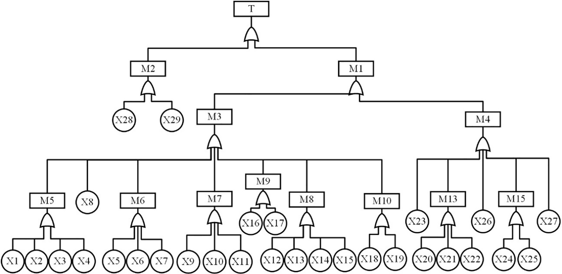
Figure 9: T-S FTA module of Shibata-type coupler system

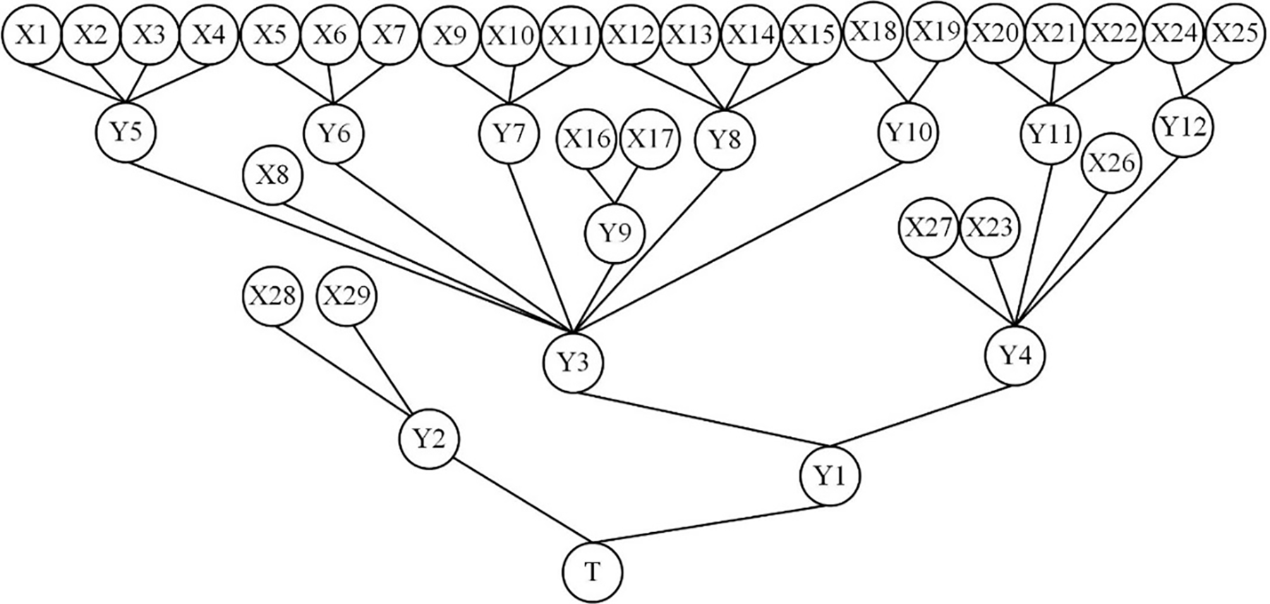
Figure 10: BN of Shibata-type coupler system

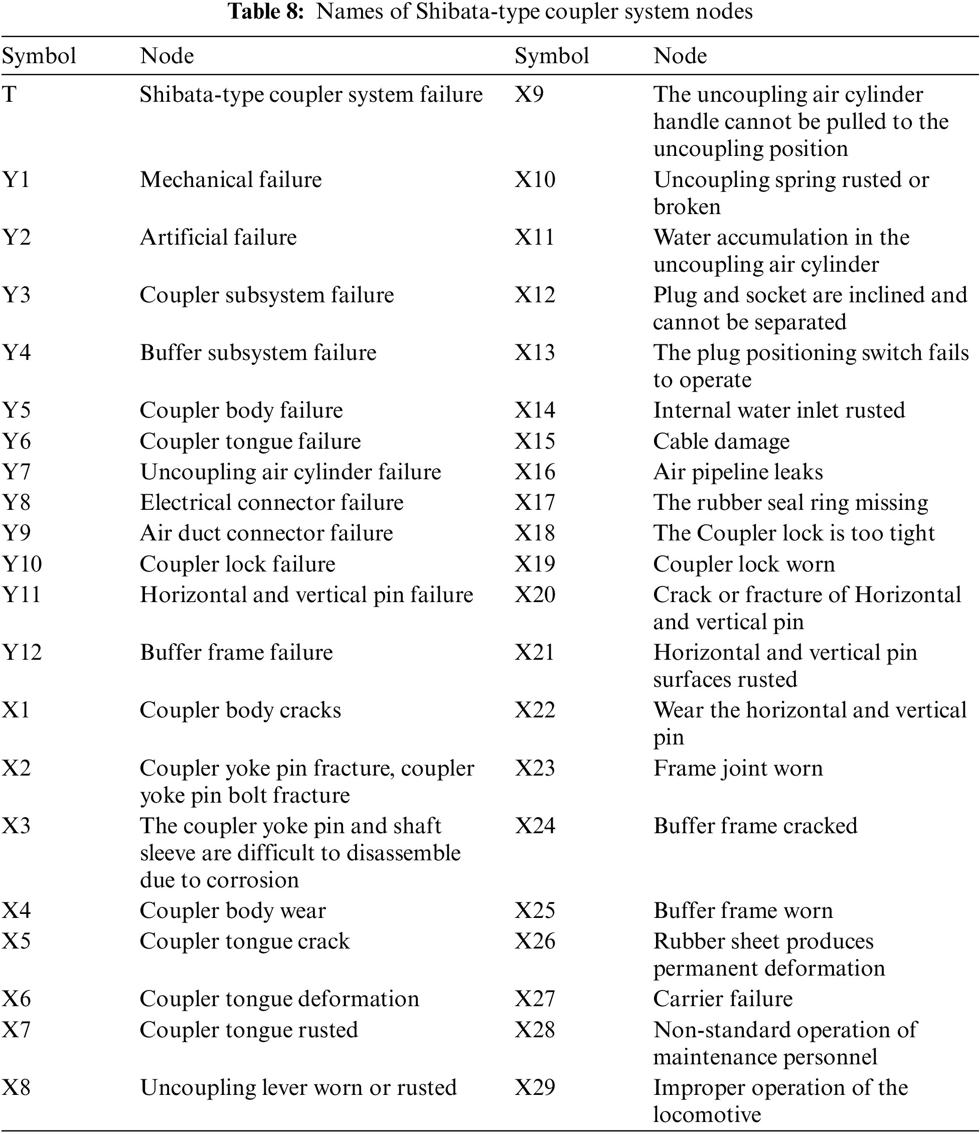
The coupler system discernment framework is Θ = {Fault occurrence, Fault non-occurrence, Fault in fuzzy uncertainty state}, which is recorded as Θ = {A1, A2, (A1,A2)}. Using the root node X1 as an example, calculate the initial failure probability interval. The expert evaluation data for root node X1 of the coupler system is shown in Table 9. Substitute it into Eqs. (6) and (7) to obtain the evidence conflict value k1 and the initial failure probability interval P(X1) of root node X1.

k1=0.00000929×0.99997089+0.00001345×0.99997822=41.5998×10−7

P(X1)=[Bel,Pl]=[0.00001345×0.00000929+0.00001345×0.00001249+ 0.00000929×0.000015661−4.15998×10−6,(0.00001345+0.00001566)×(0.00000929+0.00001249)1−4.15998×10−6]=[4.3843×10−10,6.3403×10−10]

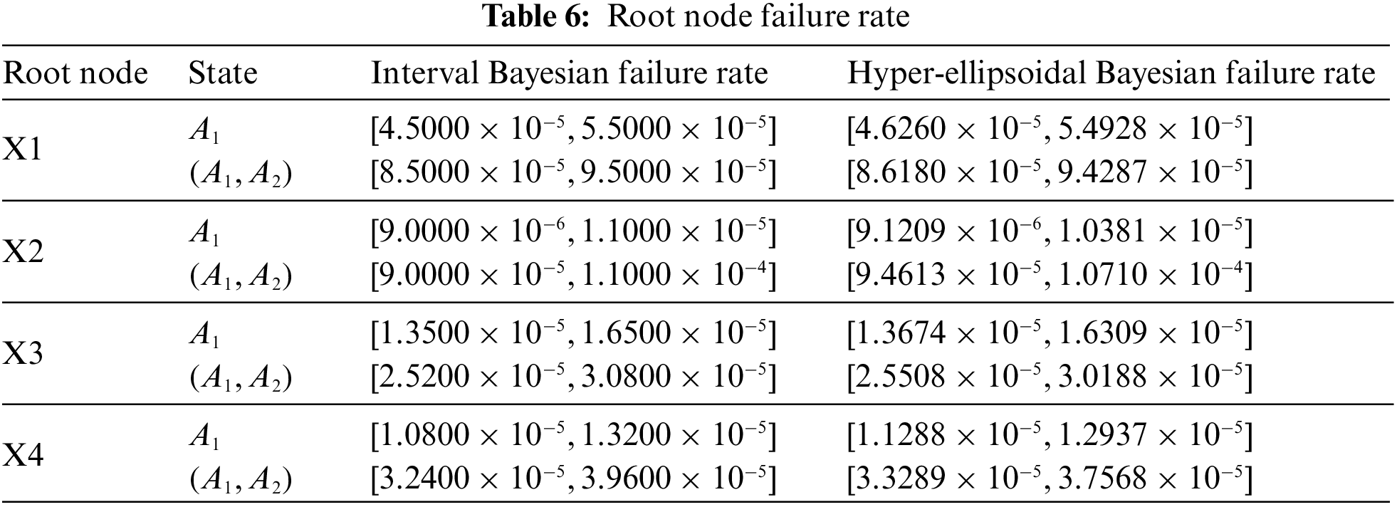
The initial failure probability interval for each root node is obtained by the same calculation as above. The root node failure probability interval after the HM constraint is obtained from Eq. (14). See Table 10 for part of this.

The T-S gate rule of the coupler system is derived from historical data and expert experience. The conditional probability table of the BN is obtained according to the method in Fig. 3. The conditional probability table for the intermediate node Y2 is shown in Table 11 as an example. Where rule 1 indicates that under the condition that X28 has a fault state of A2 and X29 has a fault state of A2, the possibility that Y2 fault state being A2 is 1, the possibility that Y2 is (A1,A2) and A1 is 0. Other rules can be used in this way.

According to the failure probability interval of X28 and X29 and Table 11, the failure probability interval of Y2 in various states can be obtained by using Eq. (15) as follows:

P(y2−A1)=∑x28,x29⁡P(x28,x29;y2=A1)=∑x28,x29⁡P(y2=A1|x28,x29)×P(x28)×P(x29)=[1.3611×10−12,1.4528×10−12]

P(y2=(A1,A2))=∑x28,x29⁡P(x28,x29;y2=(A1,A2))=∑x28,x29⁡P(y2=(A1,A2)|x28,x29)×P(x28)×P(x29)=[9.1862×10−13,9.6967×10−13]

P(y2−A2)=∑x28,x29⁡P(x28,x29;y2=A2)=∑x28,x29⁡P(y2=A2|x28,x29)×P(x28)×P(x29)=[99999999.9998×10−8,99999999.9998×10−8]

The above results show that Y2 has a small probability of a fault and a fault-indeterminate state and a high probability of no fault. This is consistent with the actual situation. Based on the constructed BN, the probability intervals of failure for leaf node T with fault states A1, (A1,A2), and A2 were found using the method and combined with the conditional probability tables of the nodes. The reliability curve of the hook system can be obtained as shown in Fig. 11. As can be seen in Fig. 11, the reliability of the coupler system is in the range [0.7873, 0.8505] after 1×108 h of operation. Based on the results of the reliability assessment of the coupler system, a basis can be provided for subsequent design and maintenance work.

P(T=A1)=[1.6663×10−10,1.4425×10−9]

P(T=(A1,A2))=[1.0585×10−9,1.4525×10−9]

P(T=A2)=[99999.9997×10−5,99999.9998×10−5]

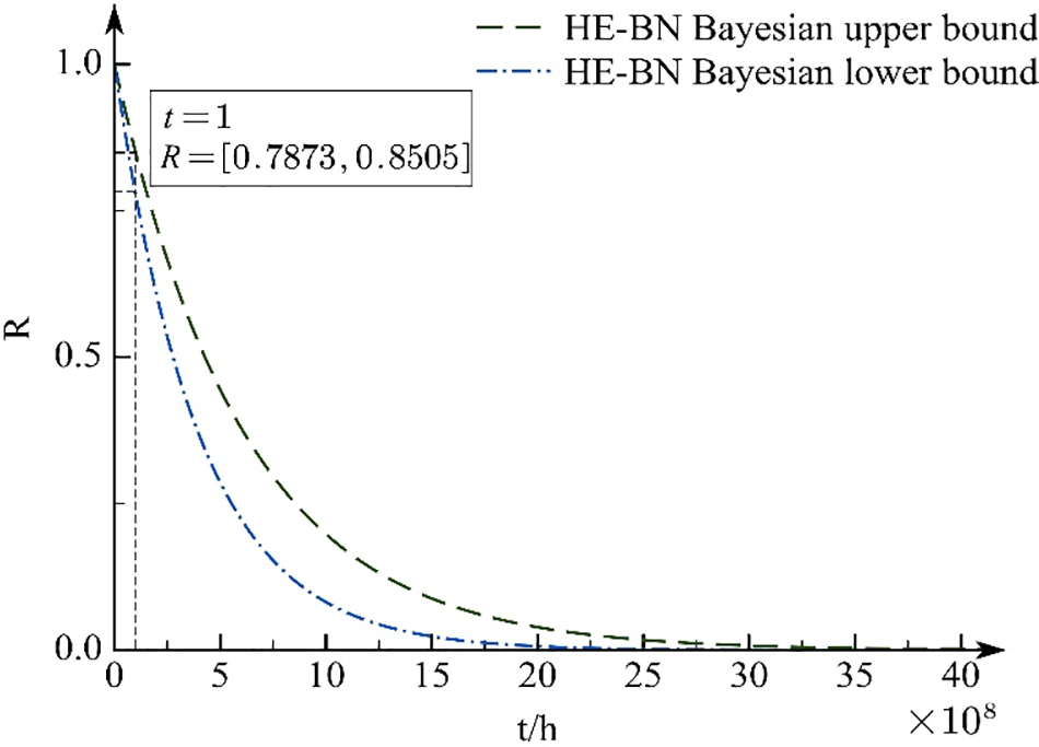
Figure 11: Coupler system reliability curve

The posterior probability of the root node xi for leaf node T with fault states A1 and (A1,A2) can be calculated according to Eq. (16). After sorting them by the interval number sorting method [33], the posterior probability is shown in Fig. 12.

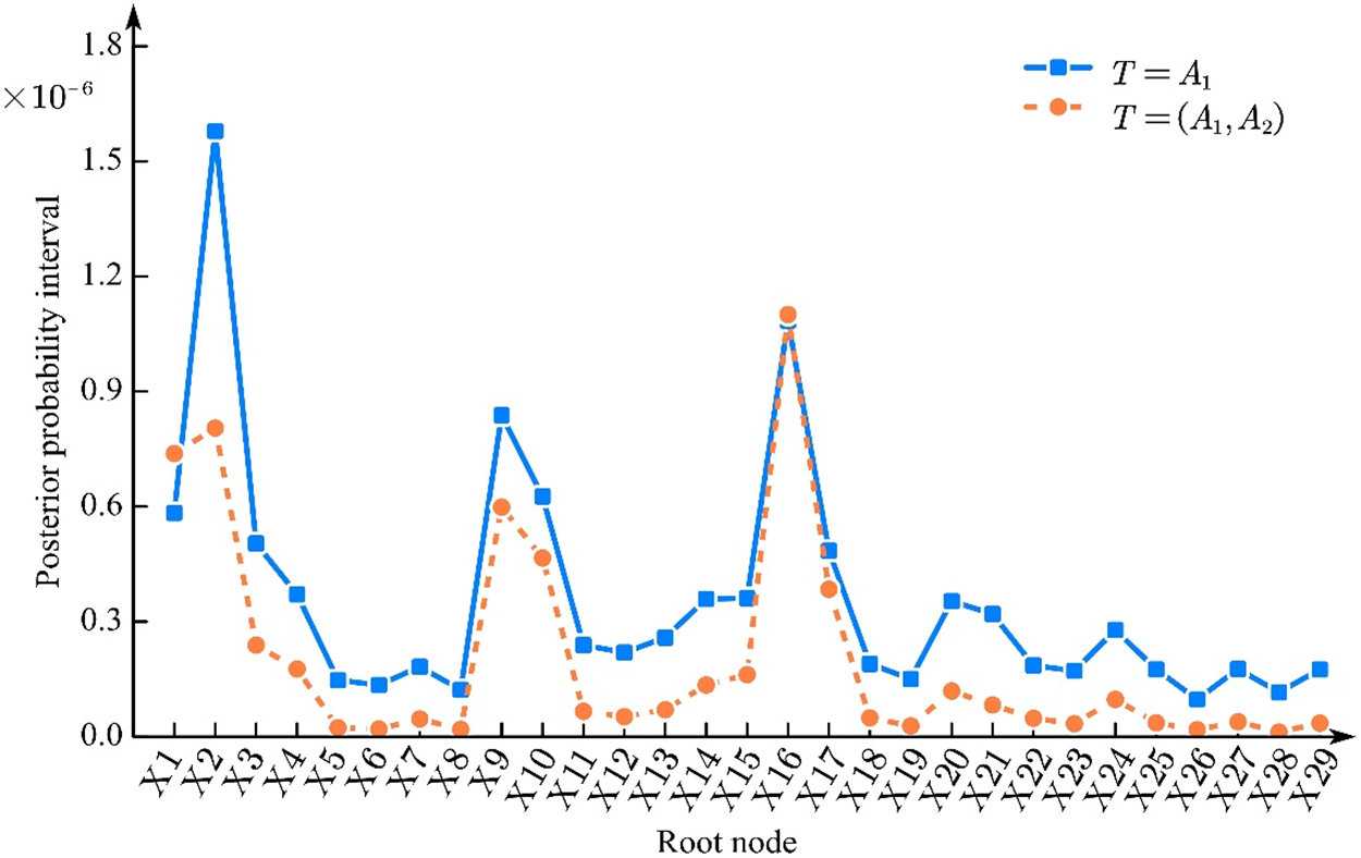
Figure 12: Posterior probability of root nodes

As can be seen from Fig. 12, when the Shibata-type coupler system fails, the root node posterior probabilities are ordered as follows:

X2>X16>X9>X10>X1>X3>X17>X4>X15>X14>X20>X21>X24>X13>X11>X12>X18>X22>X7>X27>X25>X29>X23>X19>X5>X6>X8>X28>X26.

When the fault of the Shibata-type coupler system is in a fuzzy uncertainty state, the posterior probability of the root node is sorted as follows:

X16>X2>X1>X9>X10>X17>X3>X4>X15>X14>X20>X24>X21>X13>X11>X12>X18>X22>X7>X27>X25>X29>X23>X19>X5>X6>X8>X26>X28.

A comparison of the failure rates from CRH2 and CRH30A (L) rolling stock operational data [35] with the results obtained from a reliability analysis method based on T-S FTA and HE-BN is shown in Fig. 13.

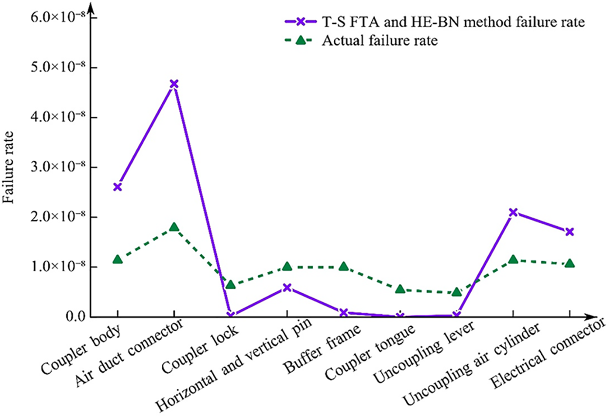
Figure 13: Result comparison

It can be seen from Fig. 13 that in the operation data of CRH2 and CRH380A (L) multiple units, the failure rate of key components of the Shibata-type coupler system is ranked as follows: air duct connector, coupler body, uncoupling air cylinder, electrical connector, horizontal and vertical pin, buffer frame, coupler lock, coupler tongue, uncoupling lever. The results are consistent with the sequence when the coupler system fault state is A1 in the reliability analysis method of the T-S FTA and HE-BN, which verifies the correctness and feasibility of the method.

The greater the posterior probability, the greater the impact of the component on the system failure, which is the weak link that the system should focus on. From the analysis results in Figs. 12 and 13, it can be seen that when the coupler system is in a (A1,A2) state, coupler yoke pin fracture and coupler yoke pin bolt fracture have the greatest impact on the system. This is followed by the Air pipeline leak and uncoupling air cylinder failure. Therefore, these components should be inspected and repaired first when the system is in a half-fault state or has reached the preventive maintenance time point to ensure longer system life. When the system is in the A1 fault state, the Air pipeline leak has the greatest impact on the system, followed by the Coupler yoke pin fracture, coupler yoke pin bolt fracture, and the Coupler body crack, and the impact of the Non-standard operation of the maintenance personnel is the smallest.

4.3 A Type of Double-Row Tapered Roller Bearing System Reliability Analysis

The structure of a bogie bearing for a moving train is shown in Fig. 14 and includes the inner ring, the outer ring, the rolling element, and the cage. The inner ring fits with the shaft and rotates with it. The outer ring fits into the bearing housing and plays a supporting role. The rolling element is evenly distributed between the inner ring and outer ring with the help of the cage. The bogie axle box bearing supports the static load of the vehicle and the longitudinal and transverse impact of the vehicle in operation and other dynamic loads, and its failure mode can be classified as rust, discoloration, surface plastic deformation, fatigue spalling and pitting failure, cracks and defects in five categories.

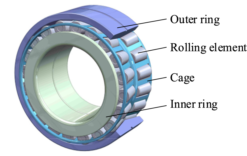
Figure 14: Bearing structure

A T-S fault tree with bearing failure as the top event was constructed for a type of double-row tapered roller bearing used in the bogie of a moving train, as shown in Fig. 15. It is transformed into a BN as shown in Fig. 16. The meanings represented by the symbols in Fig. 16 are shown in Table 12.

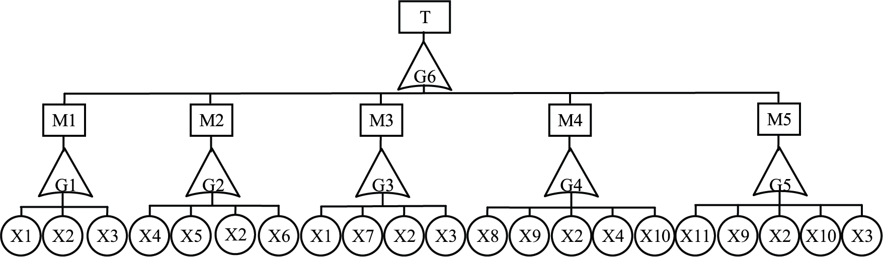
Figure 15: Bearing system T-S fault tree

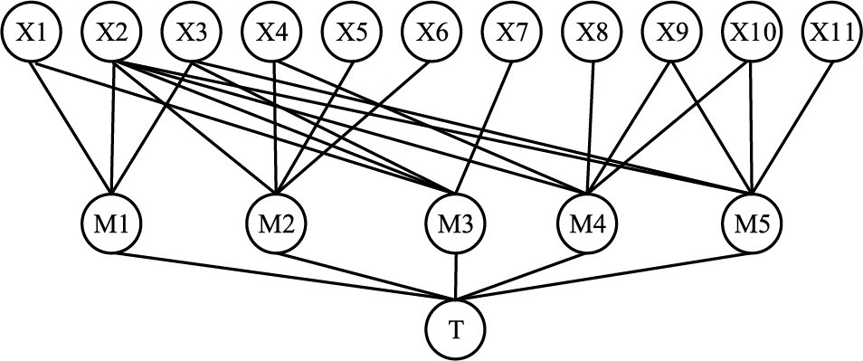
Figure 16: Bearing system Bayesian network

Define the identification framework of the bearing system as Θ = {Fault occurrence, Fault in fuzzy uncertainty state, Fault non-occurrence}, denoted as Θ = {A1, (A1,A2), A2}. Substitute the expert evaluation data of the root nodes of the bearing Bayesian network into Eqs. (6) and (7) to obtain the initial failure probability interval of each root node. The failure probability interval of the root node after the HM constraint is obtained from Eq. (14) and is shown in Table 13.

The T-S gate rule for the bearing system is derived from historical data and expert experience, and the conditional probability table for the BN is obtained according to the method in Fig. 3. Take the conditional probability table of the intermediate node M1 as an example, see Table 14.

Based on the constructed BN and the conditional probability tables of the nodes, the probability intervals of failure for leaf node T with fault states A1, (A1,A2), and A2 were found. A reliability curve for the bearing system can be obtained, as shown in Fig. 17. As can be seen in Fig. 17, the bearing system reliability interval is [0.8793, 0.8975] after 1954 h of system operation, and the reliability decreases sharply within 40,000 h of operation. Based on the results of the reliability assessment of the bearing system, a basis for subsequent design and maintenance work can be provided.

P(T=0)=[9.9987×10−1,9.9989×10−1]

P(T=0.5)=[5.4848×10−5,6.5295×10−5]

P(T=1)=[5.5327×10−5,6.5835×10−5]

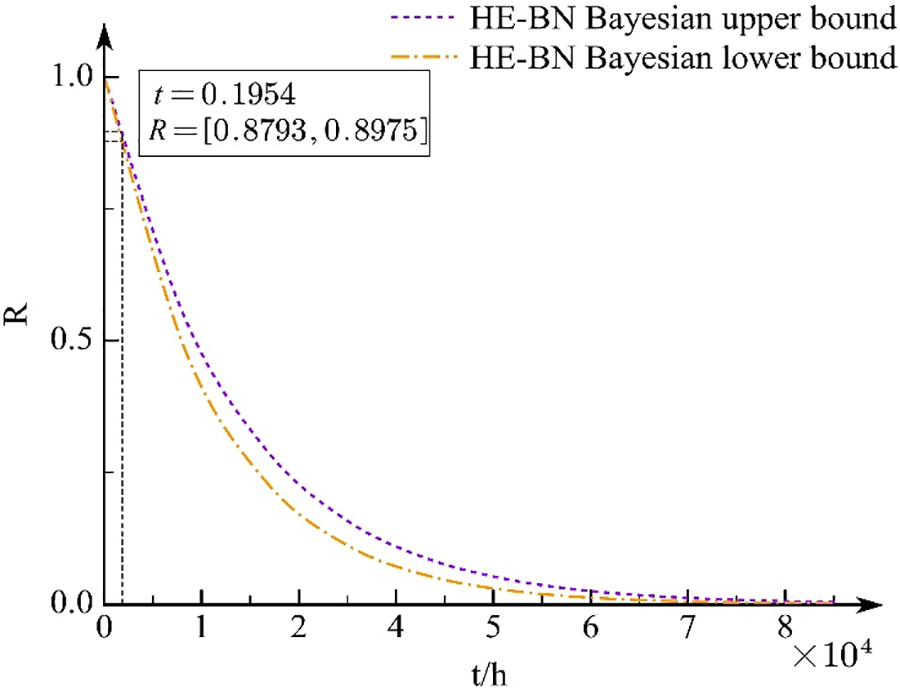
Figure 17: Bearing system reliability curve

The posterior probability of the root node xi for leaf node T with fault states A1 and (A1,A2) can be calculated according to Eq. (16). After sorting them by the interval number sorting method [33], they are shown in Fig. 18.

Figure 18: Posterior probability of the bearing system root nodes

As can be seen from Fig. 18, when the bearing system failure occurs, the root node posterior probability ranking is as follows: X1>X2>X11>X10>X9>X4>X7>X6>X8>X5>X3.

When the failure of the bearing system is in a state of fuzzy uncertainty, the root node posterior probabilities are ordered as follows: X2>X1>X11>X10>X9>X4>X7>X6>X8>X5>X3.

As can be seen in Fig. 18, X1,X2, and X8 are of greater importance. The main faults of these three basic events are poor lubrication, seal failure, and excessive impact loads. Therefore, the following improvement measures can be prioritized to improve the reliability of this bearing system.

Strengthen and improve the bearing lubrication technology, and bearing seal device maintenance, to ensure that the bearings are subject to good lubrication. In bearing maintenance, develop on-site applicable maintenance and cleaning cycles, improve the operational level of maintenance of bearings, improve maintenance conditions, and ensure the quality of bearing maintenance. In terms of bearing design, improve the structure of the bearing to increase the bearing’s impact resistance and improve the internal force condition of the bearing.

5  Conclusions

This paper proposes a system reliability analysis method based on T-S FTA and HE-BN. Combining the advantages of T-S FTA and BN, directed acyclic graphs and conditional probability tables of BN are constructed through T-S gates and T-S rules. Evidence theory and the HM are applied to obtain the fault interval of the system BN root node. The fault interval of the system is obtained by forward calculation based on the directed acyclic graph, the conditional probability table, and the fault interval of the root node. The reverse calculation is then carried out to identify the weak points of the system. The following conclusions were obtained:

(1)   Constructing directed acyclic graphs and conditional probability tables for BN by T-S gates and T-S rules. Combines the advantages of simple T-S FTA modeling and easy BN computation. The disadvantage is solved that the BN constructed by traditional fault trees cannot describe the fuzzy logical relationship between nodes. It also solves the shortcomings of the T-S FTA which is complex in operation and cannot reason in both directions. The modeling and computational efficiency of the coupler system reliability model are improved.

(2)   The D-S evidence theory is used to fuse expert experience to obtain the failure probability interval for the BN root nodes. The HM is introduced to define the range of values of the uncertainty probability. It can effectively deal with the problems of insufficient failure data and uncertainty of failure degree. And it solves the problem that the calculation results are relatively conservative when the traditional fuzzy interval model describes the uncertain failure mechanism and data. It is more in line with engineering practice.

(3)   The application of the proposed method to a real engineering case study shows that the proposed method can establish a reliability model that is easy to calculate and fully reflects the failure characteristics of a complex structural system by integrating the failure modes and causes of the system when dealing with the reliability analysis of a multi-state complex system. It can accurately identify the weak points of the system under the uncertainty and incompleteness of the data.

In addition, the system reliability analysis method based on the T-S FTA and HE-BN proposed in this paper can be applied to other subsystems of rail vehicles, aerospace, and other fields. It can quantify the reliability level of the system, effectively identify the weak links, and has generality. However, this paper only considers the structural complexity of the system, the uncertainty and incompleteness of the data, and the polymorphic nature of the degree of component failure. A reliability analysis method that considers the dynamic characteristics of the system in operation and fault correlation could be the next step in the research.

Acknowledgement: Thanks to the help of four anonymous reviewers and journal editors, the logical organization and content quality of this paper have been improved.

Funding Statement: This work is supported by the National Natural Science Foundation of China (51875073).

Author Contributions: The authors confirm contribution to the paper as follows: study conception and design: Xia Q., Li Y.; data collection: Wang Y.; analysis and interpretation of results: Xia Q., Zhang D.; draft manuscript preparation: Xia Q., Li Y. All authors reviewed the results and approved the final version of the manuscript.

Availability of Data and Materials: All data generated or analysed during this study are included in this published article.

Conflicts of Interest: The authors declare that they have no conflicts of interest to report regarding the present study.

References

1. Meng, D. B., Yang, S. Y., De Jesus, A. M., Fazeres-Ferradosa, T., Zhu, S. P. (2023). A novel hybrid adaptive Kriging and water cycle algorithm for reliability-based design and optimization strategy: Application in offshore wind turbine monopole. Computer Methods in Applied Mechanics and Engineering, 412, 116083. https://doi.org/10.1016/j.cma.2023.116083 [Google Scholar] [CrossRef]

2. Meng, D. B., Yang, S. Y., de Jesus, A. M., Zhu, S. P. (2023). A novel Kriging-model-assisted reliability-based multidisciplinary design optimization strategy and its application in the offshore wind turbine tower. Renewable Energy, 203, 407–420. https://doi.org/10.1016/j.renene.2022.12.062 [Google Scholar] [CrossRef]

3. Meng, D. B., Yang, S. Y., He, C., Wang, H. T., Lv, Z. Y. et al. (2022). Multidisciplinary design optimization of engineering systems under uncertainty: A review. International Journal of Structural Integrity, 13(4), 565–593. https://doi.org/10.1108/IJSI-05-2022-0076 [Google Scholar] [CrossRef]

4. Yang, S. Y., Meng, D. B., Wang, H. T., Chen, Z. P., Xu, B. (2023). A comparative study for adaptive surrogate-model-based reliability evaluation method of automobile components. International Journal of Structural Integrity, 14(3), 498–519. https://doi.org/10.1108/IJSI-03-2023-0020 [Google Scholar] [CrossRef]

5. Zhi, P. P., Wang, Z. L., Chen, B. Z., Sheng, Z. Q. (2022). Time-variant reliability-based multi-objective fuzzy design optimization for anti-roll torsion bar of EMU. Computer Modeling in Engineering & Sciences, 131(2), 1001–1022. https://doi.org/10.32604/cmes.2022.019835 [Google Scholar] [CrossRef]

6. Meng, D. B., Hu, Z. G., Guo, J. B., Lv, Z. Y., Xie, T. W. et al. (2021). An uncertainty-based structural design and optimization method with interval Taylor expansion. Structures, 33, 4492–4500. https://doi.org/10.1016/j.istruc.2021.07.007 [Google Scholar] [CrossRef]

7. Liu, X., Kuang, Z. X., Yin, L. R., Hu, L. (2017). Structural reliability analysis based on probability and probability box hybrid model. Structural Safety, 68, 73–84. https://doi.org/10.1016/j.strusafe.2017.06.002 [Google Scholar] [CrossRef]

8. Mahrad, D., Mahdi, F., Hamed, Y. (2020). Failure assessment logic model (FALMA new approach for reliability analysis of satellite attitude control subsystem. Reliability Engineering and System Safety, 198, 106889. https://doi.org/10.1016/j.ress.2020.106889 [Google Scholar] [CrossRef]

9. Yi, X. J., Dhillon, B. S., Shi, J., Mu, H. N., Zhang, Z. (2017). A new reliability analysis method for vehicle systems based on goal-oriented methodology. Proceedings of the Institution of Mechanical Engineers,Part D: Journal of Automobile Engineering, 231(8), 1066–1095. https://doi.org/10.1177/0954407016671276 [Google Scholar] [CrossRef]

10. Vicenzutti, A., Menis, R., Sulligoi, G. (2019). All-electric ship-integrated power systems: Dependable design based on fault tree analysis and dynamic modeling. IEEE Transactions on Transportation Electrification, 5(3), 812–827. https://doi.org/10.1109/TTE.2019.2920334 [Google Scholar] [CrossRef]

11. Song, H., Zhang, H. Y., Chan, C. W. (2009). Fuzzy fault tree analysis based on T-S model with application to INS/GPS navigation system. Soft Computing, 13(1), 31–40. https://doi.org/10.1007/s00500-008-0290-3 [Google Scholar] [CrossRef]

12. Sun, L. N., Huang, N., Wu, W. Q., Li, X. K. (2016). Performance reliability of polymorphic systems by fuzzy fault tree based on T-S model. Journal of Mechanical Engineering, 52(10), 191–197. https://doi.org/10.3901/JME.2016.10.191 [Google Scholar] [CrossRef]

13. Li, C. Y., Sun, X. M., Jiang, X., Chen, F. J., Zhang, G. H. (2021). Analysis of the reliability of household air conditioners based on the T-S fuzzy fault tree. Journal of Machine Design, 38(2), 120–126. https://doi.org/10.13841/j.cnki.jxsj.2021.02.018 [Google Scholar] [CrossRef]

14. Liang, F., Wang, Z. (2017). The reliability analysis of welding robots based on T-S fuzzy fault tree. Journal of Mechanical Strength, 39(3), 592–597. https://doi.org/10.16579/j.issn.1001.9669.2017.03.016 [Google Scholar] [CrossRef]

15. Wang, C., Wang, L. D., Chen, H., Yang, Y. Y., Li, Y. (2021). Fault diagnosis of train network control management system based on dynamic fault tree and Bayesian network. IEEE Access, 9, 2618–2632. https://doi.org/10.1109/ACCESS.2020.3046681 [Google Scholar] [CrossRef]

16. Zhang, Z. H., Wang, Y. R., Dang, J. W. (2020). Reliability analysis of the on-board subsystem of the train control system based on evidence theory and Bayesian network method. Journal of Railway Science and Engineering, 17(9), 2208–2215. https://doi.org/10.19713/j.cnki.43-1423/u.T20200260 [Google Scholar] [CrossRef]

17. Hamza, Z., Abdallah, T. (2016). Mapping fault tree into Bayesian network in safety analysis of process system. 2015 4th International Conference on Electrical Engineering, pp. 1–5. Boumerdes, Algeria.https://doi.org/10.1109/INTEE.2015.7416862 [Google Scholar] [CrossRef]

18. Bai, X., Tang, R. J., Luo, X. F., Sun, L. P. (2020). Multi-state reliability analysis of semi-submersible drilling rig system based on fault tree analysis and Bayesian network method. China Shipbuilding, 61(2), 220–228. https://doi.org/10.3969/j.issn.1000-4882.2020.02.021 [Google Scholar] [CrossRef]

19. Mi, J. H., Li, Y. F., Peng, W. W., Huang, H. Z. (2018). Reliability modeling and analysis of complex multi-state system based on interval fuzzy Bayesian network. Science China Physics, Mechanics & Astronomy, 48(1), 54–66. https://doi.org/10.1360/SSPMA2016-00521 [Google Scholar] [CrossRef]

20. Pan, Y., Zhang, L. M., Li, Z. W., Ding, L. Y. (2020). Improved fuzzy Bayesian network-based risk analysis with interval-valued fuzzy sets and D–S evidence theory. IEEE Transactions on Fuzzy Systems, 28(9), 2063–2077. https://doi.org/10.1109/TFUZZ.2019.2929024 [Google Scholar] [CrossRef]

21. Zhang, G. Z., Thai, V. V., Yuen, K. F., Loh, H. S., Zhou, Q. J. (2018). Addressing the epistemic uncertainty in maritime accidents modelling using Bayesian network with interval probabilities. Safety Science, 102, 211–225. https://doi.org/10.1016/j.ssci.2017.10.016 [Google Scholar] [CrossRef]

22. Wu, C. Y., Wang, H. C. (2018). Fault analysis of T-S fuzzy causality diagram under hyper-ellipsoidal model. Journal of Chongqing Technology and Business University (Natural Science Edition), 35(6), 27–33. https://doi.org/10.16055/j.issn.1672-058X.2018.0006.006 [Google Scholar] [CrossRef]

23. Qiu, Z. P., Hu, Y. M. (2016). The relations of non-probabilistic reliability measures based on ellipsoidal convex model and interval safety factors. Chinese Journal of Computational Mechanics, 33(4), 522–527. https://doi.org/10.7511/jslx201604016 [Google Scholar] [CrossRef]

24. Ouyang, H., Liu, J., Han, X., Liu, G. R., Ni, B. Y. et al. (2020). Correlation propagation for uncertainty analysis of structures based on a non-probabilistic ellipsoidal model. Applied Mathematical Modelling, 88, 190–207. https://doi.org/10.1016/j.apm.2020.06.009 [Google Scholar] [CrossRef]

25. Sun, W. C., Yang, Z. C., Li, K. F. (2013). Non-deterministic fatigue life analysis using convex set models. Science China Physics. Mechanics & Astronomy, 56, 765–774. https://doi.org/10.1007/s11433-013-5023-7 [Google Scholar] [CrossRef]

26. Li, K., Liu, H. W. (2022). Structural reliability analysis by using non-probabilistic multi-cluster ellipsoidal model. Entropy, 24(9), 1209. https://doi.org/10.3390/e24091209 [Google Scholar] [PubMed] [CrossRef]

27. Yao, C. Y., Lv, J., Chen, D. N., Li, S. (2015). Convex model T-S fault tree and importance analysis method. Journal of Mechanical Engineering, 51(24), 184–192. https://doi.org/10.3901/JME.2015.24.184 [Google Scholar] [CrossRef]

28. Zhang, F., Wang, Y. M., Gao, Y., Xu, X. Y., Cheng, L. (2019). Fault tree analysis of an airborne refrigeration system based on a hyper-ellipsoidal model. IEEE Access, 7, 139161–139171.https://doi.org/10.1109/ACCESS.2019.2942351 [Google Scholar] [CrossRef]

29. Zhang, L. L., He, Y. X., Zhai, W. H., Zhao, J. Y., Zhang, F. (2017). Fault tree analysis of aircraft hydraulic brake system based on hyper-ellipsoidal model. Mechanical Strength, 39(4), 842–847. https://doi.org/10.16579/j.issn.1001.9669.2017.04.017 [Google Scholar] [CrossRef]

30. Chen, X. Y., Fan, J. P., Bian, X. Y. (2017). Structural robust optimization design based on convex model. Results in Physics, 7, 3068–3077. https://doi.org/10.1016/j.rinp.2017.08.013 [Google Scholar] [CrossRef]

31. Yang, S. Y., Wang, J. P., Yang, H. F. (2022). Evidence theory based uncertainty design optimization for planetary gearbox in wind turbine. Journal of Advances in Applied & Computational Mathematics, 9, 86–102. https://doi.org/10.15377/2409-5761.2022.09.7 [Google Scholar] [CrossRef]

32. Liu, G. Y., Zhang, C. Y. (2019). Reliability analysis of improved Bayesian network hydraulic system based on evidence theory. Machine Tool & Hydraulics, 47(24), 17–23. https://doi.org/10.3969/j.issn.1001-3881.2019.24.004 [Google Scholar] [CrossRef]

33. Li, D. Q., Zeng, W. Y., Yin, Q. (2020). Overview of interval number ranking methods. Journal of Beijing Normal University, 56(4), 483–492. https://doi.org/10.12202/j.0476-0301.2019155 [Google Scholar] [CrossRef]

34. Yin, T. (2019). Height adjustment of Shibata front-end coupler. Rail Transportation Equipment and Technology, 2, 50–52. https://doi.org/10.13711/j.cnki.cn32-1836/u.2019.02.019 [Google Scholar] [CrossRef]

35. Zheng, W. (2018). Analysis of the expected RAM of the hook retarder (Shibata type) for moving trains. Rail Transportation Equipment and Technology, 269(4), 6–9. https://doi.org/10.13711/j.cnki.cn32-1836/u.2018.04.003 [Google Scholar] [CrossRef]