
 Submit a Paper
 Propose a Special lssue
 Open Access
ARTICLE
A Stochastic Model to Assess the Epidemiological Impact of Vaccine Booster Doses on COVID-19 and Viral Hepatitis B Co-Dynamics with Real Data
1 Department of Mathematics, Federal University of Technology, Owerri, 460114, Nigeria
2 Abdus Salam School of Mathematical Sciences, Government College University, Lahore, 54000, Pakistan
3 Department of Mathematics, Government College University, Lahore, 54000, Pakistan
4 Department of Computer Science and Mathematics, Labanese American University, Beirut, Lebanon
5 Institute of Space Sciences, Magurele-Bucharest, Romania
6 Department of Medical Research, China Medical University Hospital, China Medical University, Taichung, 40402, Taiwan
* Corresponding Author: Andrew Omame. Email:
(This article belongs to the Special Issue: Mathematical Aspects of Computational Biology and Bioinformatics-II)
Computer Modeling in Engineering & Sciences 2024, 138(3), 2973-3012. https://doi.org/10.32604/cmes.2023.029681
Received 02 March 2023; Accepted 04 August 2023; Issue published 15 December 2023
 View Full Text
 Download PDF
Abstract
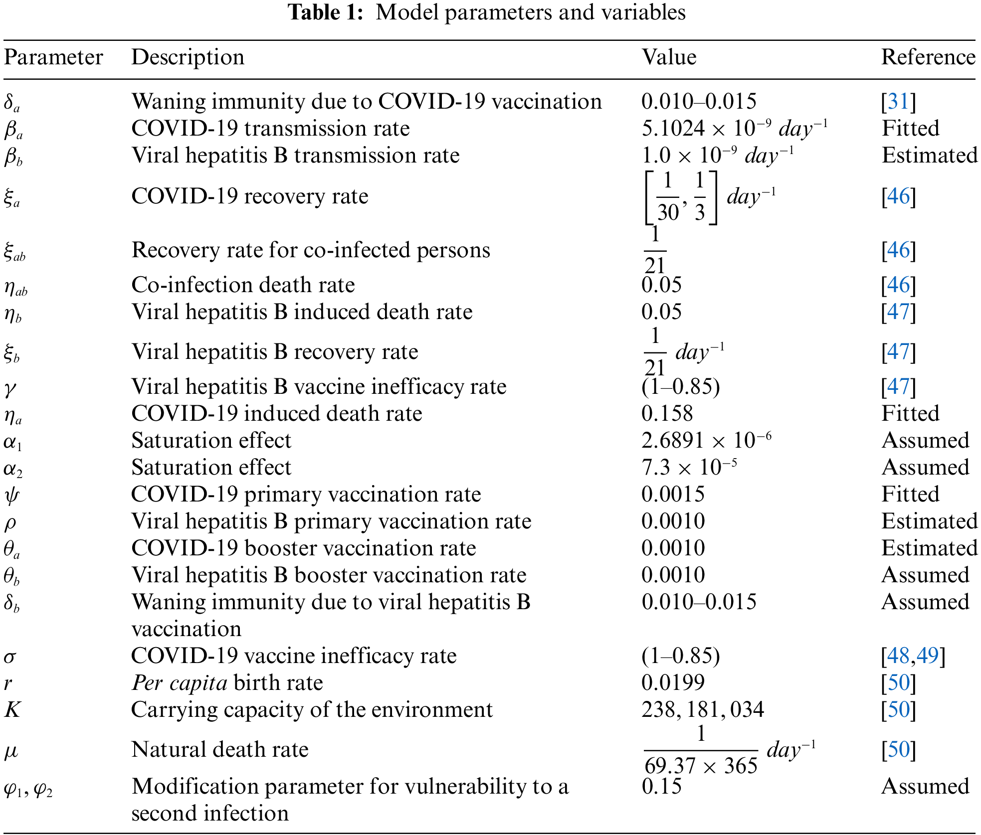
A patient co-infected with COVID-19 and viral hepatitis B can be at more risk of severe complications than the one infected with a single infection. This study develops a comprehensive stochastic model to assess the epidemiological impact of vaccine booster doses on the co-dynamics of viral hepatitis B and COVID-19. The model is fitted to real COVID-19 data from Pakistan. The proposed model incorporates logistic growth and saturated incidence functions. Rigorous analyses using the tools of stochastic calculus, are performed to study appropriate conditions for the existence of unique global solutions, stationary distribution in the sense of ergodicity and disease extinction. The stochastic threshold estimated from the data fitting is given by: . Numerical assessments are implemented to illustrate the impact of double-dose vaccination and saturated incidence functions on the dynamics of both diseases. The effects of stochastic white noise intensities are also highlighted.Keywords
According to the report issued on April 24, 2023, by Johns Hopkins University Coronavirus Center: The “Coronavirus Disease 2019” (COVID-19) caused by the “Severe Acute Respiratory Syndrome Coronavirus-2” (SARS-CoV-2) has infected 676,609,955 individuals which resulted in 6,881,955 deaths globally, and 13,338,833,198 COVID-19 vaccine doses have been administered [1]. Viral hepatitis B virus (HBV) poses a great threat to public health globally [2]. The “Centers for Disease Control and Prevention” has estimated that over 290 million individuals are infected with HBV with nearly 0.9 million deaths globally [3]. HBV is among the high-risk factors for chronic liver infections: cirrhosis, liver fibrosis and hepatocellular carcinoma. It is worth mentioning that HBV is responsible for more than 40% of hepatocellular carcinoma cases and more than 25% of liver cirrhosis cases [4]. The “Global Burden of Disease” has reported that HBV infection is one of the leading causes of adult mortality worldwide with more than 750,000 deaths annually associated with it [5]. The prevalence of HBV cases differs across different countries and regions [6]. Most HBV cases have been reported in the Middle East countries, Asia, and Africa [7]. In many of these countries, most of the reported cases are transmitted via mother-child [7]. Particularly, in Pakistan, the prevalence of viral hepatitis B is around 5 million [8]. Recent studies have indicated that between 2% and 11% of individuals infected with COVID-19 were already suffering from the liver infection and about 25% of liver problems are linked with COVID-19 [9]. SARS-CoV-2 infection can be a big risk factor for severe illness among under-diagnosed patients with viral hepatitis B [10].
According to the report issued by the “McGill COVID-19 vaccine tracker” system on December 02, 2022; 50 out of 242 developed vaccines were approved and are now available in over 200 countries [11]. Some of the approved against COVID-19 include: “BNT162b2 (Pfizer/BioNTech), AZD-1222/ChAdOx1-nCoV (Oxford/AstraZeneca), NVX-CoV2373 (Novavax), CoronaVac (Sinovac), mRNA-1273 (Moderna), rAd26-S+rAd5-S (Sputnik V), and Ad26.COV2.S (Janssen)” [12]. The effectiveness of many recommended vaccines ranges between 60% and above 90% [12]. Although antiviral agents can treat HBV, medicines alone cannot eradicate the virus from a host. Thus, vaccination has become an important resource to eliminate HBV infections [13]. That is why, different countries like China and the USA have made infant and adult vaccination programme a government priority [13,14]. This measure has significantly reduced the prevalence of HBV, as reported by Zheng et al. [14] and Zhao et al. [13]. However, developing nations in Asia and sub-Saharan Africa are still far away from achieving the target of mass vaccination, especially among the adult population.
On the other hand, mathematical modeling play a significant role not only in understanding the dynamics of the disease but also in suggesting the cost effective measures to eliminate the disease. Different epidemiological models have been proposed and analyzed to understand the dynamics of COVID-19 [15–21], Hepatitis B virus [22,23] as well as the co-infection both diseases [24–26]. Specifically, the authors [24] considered an HBV-COVID-19 model in resource limitation settings. Omame et al. [25] investigated the impact of incident co-infection in a model for HBV and COVID-19, and showed that this phenomenon could trigger backward bifurcation. Din et al. [26] investigated a co-dynamical model for HBV and COVID-19 with a bilinear incidence rate. Mathematical modelling can mainly be classified into deterministic and stochastic modelling. Though, deterministic models have their own merits and advantages but stochastic models have a potential to incorporate uncertainties and randomness and to explain the dynamics of epidemics more effectively. This is why, stochastic models have been applied successfully in understanding the patterns of diseases in recent years [27–32].
As a matter of fact, the nature of epidemic growth and spread is random due to the unpredictability in human-to-human contacts [33]. Therefore, handling the variability and randomness in the different states of the disease dynamical system is a big challenge [34] (see also, [35]). In many such cases, stochastic models could best describe the randomness of infectious contacts which takes place at different infectious stages [36]. It has been shown that stochastic models provide a higher level of realistic outputs when compared with their deterministic counterparts [37]. It was shown in [37] that an endemic equilibrium appearing in a deterministic model could disappear in its corresponding stochastic model because of stochastic fluctuations. Also, the authors in [38] explained that stochastic models give better interpretation to the question of disease extinction than their deterministic equivalents. Nasell [39] pointed out that stochastic models present better approaches in describing epidemics given large range of realistic parameter values when compared with the corresponding deterministic models.
Vaccination has become an important measure in managing the co-spread of both COVID-19 and viral hepatitis B; a feature that has not been considered by previous studies. This is the main motivation behind this work which aims to fill the gap in the existing studies by proposing a robust stochastic model for the two viral diseases co-dynamics incorporating vaccine booster doses, logistic growth and saturated incidence rates. The logistic growth deals with the population growth over time taking the carrying capacity into consideration when there is limited resources whereas, in exponential growth assumption, the population of interest grows over time and the carrying capacity is not considered which is not realistic and hence the logistic growth is most suitable [40]. Also, effective contacts between infected and uninfected humans may saturate at high infection peaks as a result of the crowding effect of infected individuals or as a result of control measures by the uninfected individuals [41]. The saturated incidence function best explains this, and has been adopted successfully in many epidemic models [42–44]. In biological models which deal with high co-endemicity of two diseases, this serves as the best incidence rate.
This study develops and analyzes the model using stochastic calculus tools. It seeks to suggest comprehensive intervention measures against the two viral diseases with the inclusion of vaccination programs for both infections. The study’s findings contribute significantly to aid in the battle against COVID-19 and viral hepatitis.
This paper contributes in the following:
(i) A novel comprehensive stochastic model incorporating the logistic growth and saturated incidence rates is designed to assess the epidemiological effect of vaccine booster doses on the co-dynamics of viral hepatitis B and COVID-19.
(ii) The perturbed system is fitted to the real data from Pakistan and stochastic thresholds for both diseases are estimated.
(iii) Rigorous analysis using the tools of stochastic calculus are performed to establish appropriate conditions needed for existence of unique global solution, stationary distribution in the sense of ergodicity and disease extinction.
(iv) The optimal levels for COVID-19 and viral hepatitis B primary and booster vaccination rates that eliminate both infections are determined.
(v) Numerical assessments are carried out which highlight the impact of saturated incidence functions and stochastic white noise intensities on the dynamics of both diseases.
We shall now recall some basic tools of stochastic calculus required in the sequel.
Theorem 1.1. [45] Let
where,
The “infinitesimal generator”
Lemma 1.1. [45] If
Also, the one dimensional Ito’s lemma [44] can be re-written as:
The compartments for the formulation of the proposed model are defined as follows:
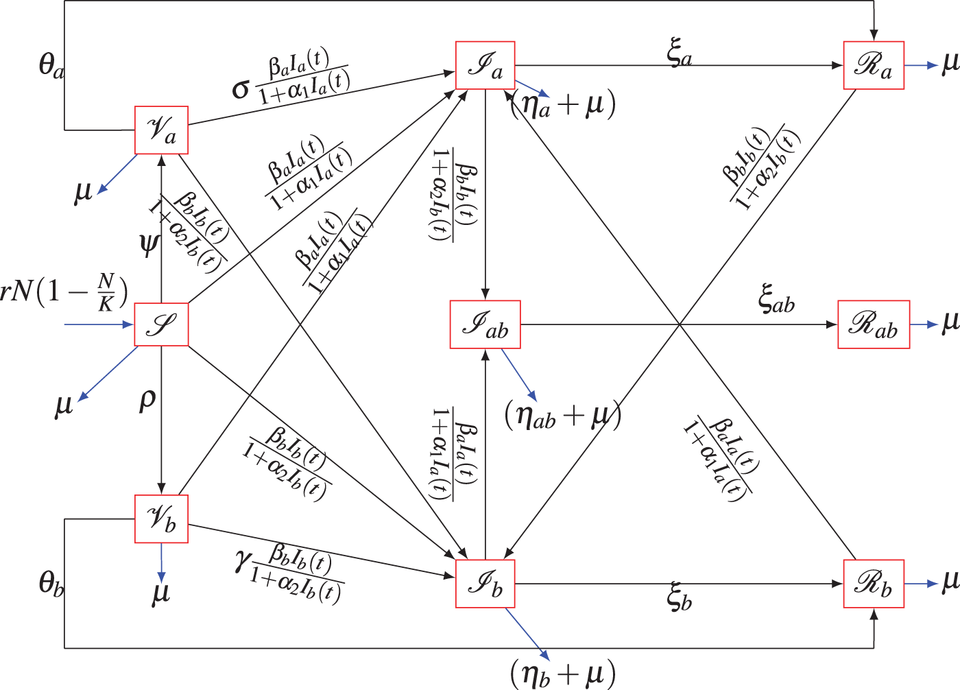
Figure 1: Model’s schematic diagram
The stochastic model analogue of the above deterministic model is given by:
where,
3 Analysis of the Unperturbed System (6)
In this section, we now present the analysis of the unperturbed system (6).
3.1 Unperturbed System’s Reproduction Number
The disease free equilibrium (DFE) for the deterministic system is:
with,
Associated transfer matrices are:
The basic reproduction employing the approach in [51] is:
3.2 Local Asymptotic Stability the Unperturbed System’s DFE (6)
Theorem 3.1. The unperturbed system’s DFE,
Proof:
Note that, the stability within neighbourhood of DFE for unperturbed system (6) is analyzed with the help of its Jacobian matrix evaluated at DFE given by:
where,
The first seven eigenvalue are given by:
and the solutions of these equations:
As all parameters of the model are positive, it is concluded that the equations in (11) will both possess roots with negative real parts whenever
4 Analysis of the Perturbed System (6)
In this section, we study appropriate conditions for the existence of a unique global solution to the stochastic system with the help of well defined stochastic Lyapunov functions. We now present the following result:
Theorem 4.1. Given the initial conditions
the perturbed system (7) has a unique global solution
for
Proof:
For given initial states
Note that,
If
Define a
Applying Ito’s lemma [45] to (14), we have
On simplification, we obtain that
Hence,
where,
Thus, we have
If both sides of Eq. (16) are integrated from
On taking expectation on both sides of the above inequality, we obtain that
Let
is not less than
Therefore,
Finally, we have
where,
The following notation and results are stated first:
Theorem 4.2 (“Strong Law of Large Numbers”). [45] Let
Lemma 4.1. Let
Moreover, if
This Proof follows using the arguments similar to those given in Lemmas
The threshold parameter
where,
The theorem below provides necessary requirement for disease extinction from a population.
Theorem 4.3. Given the initial states
(a) (i)
(ii)
(b) (i)
(ii)
Thus, if the requirements (a) and (b) above are satisfied, then
That is, both viral diseases will be eliminated with probability one.
More-over,
Proof:
(a) If
Re-writing (24) in the form of integral gives that
This can also be written in the form given by:
Dividing by
Using the “Strong Law of Large numbers”,
That is,
Similarly, it can be shown that
which implies that
(b) Also, if Eq. (24) is integrated over the interval
Moreover,
If
Eq. (28) implies
Applying
Note that
If
Eq. (32) gives
Using the last equation of the stochastic system, we have
From the first equations of system (7), we get that
Considering the bound for N, and recalling (29) and (33), gives
Dividing by
which can be re-written as:
On taking
Following the similar arguments to those given above, the following expressions can also be obtained from the stochastic system (7):
Solving the Eqs. (38) and (39) simultaneously, the following bounds are obtained
4.3 Existence of Ergodic Stationary Distribution
Definition 4.1. [52] “The transition probability function
Let
The corresponding diffusion matrix is defined as:
Lemma 4.2. [52] “Suppose there exists a bounded open domain
A1: “there exists a positive number G such that
A2: “there exists a non-negative
“Then the Markov process
with
Theorem 4.4. Define the threshold
where,
Then the perturbed system (7) has a “unique ergodic stationary distribution”
Proof:
For
Suppose that
where,
Then we have
Therefore, the requirement A1 of Lemma (4.2) is fulfilled.
Now, consider a
Let
where
Thus, we get that
Since the arithmetic mean is always greater than or equal to the geometric mean, it implies that
where,
Let
with
Consequently, we have
It implies that
Moreover, define
where,
Now, consider a
Applying Ito’s Lemma, we have
which results in
where,
Define the domain
where
Next, we show that
Case 1. Suppose
If
Similarly, it can also be shown that
Case 2. If
If we take,
Similarly, we can obtain that
Hence, there exist
Therefore, we have
Let
Taking expectation, applying Dynkin’s formula [53] and integrating both sides of Eq. (50) over
Since
Following arguments similar to those in the proof of the Theorem (4.4), we can show that
Now,
5 Numerical Scheme/Simulations
The perturbed system (7) shall now be experimented numerically in this section. The higher order scheme by Milstein [55] shall be used and is defined below:
with,
Figure 2: Fitting of the proposed stochastic model to real data
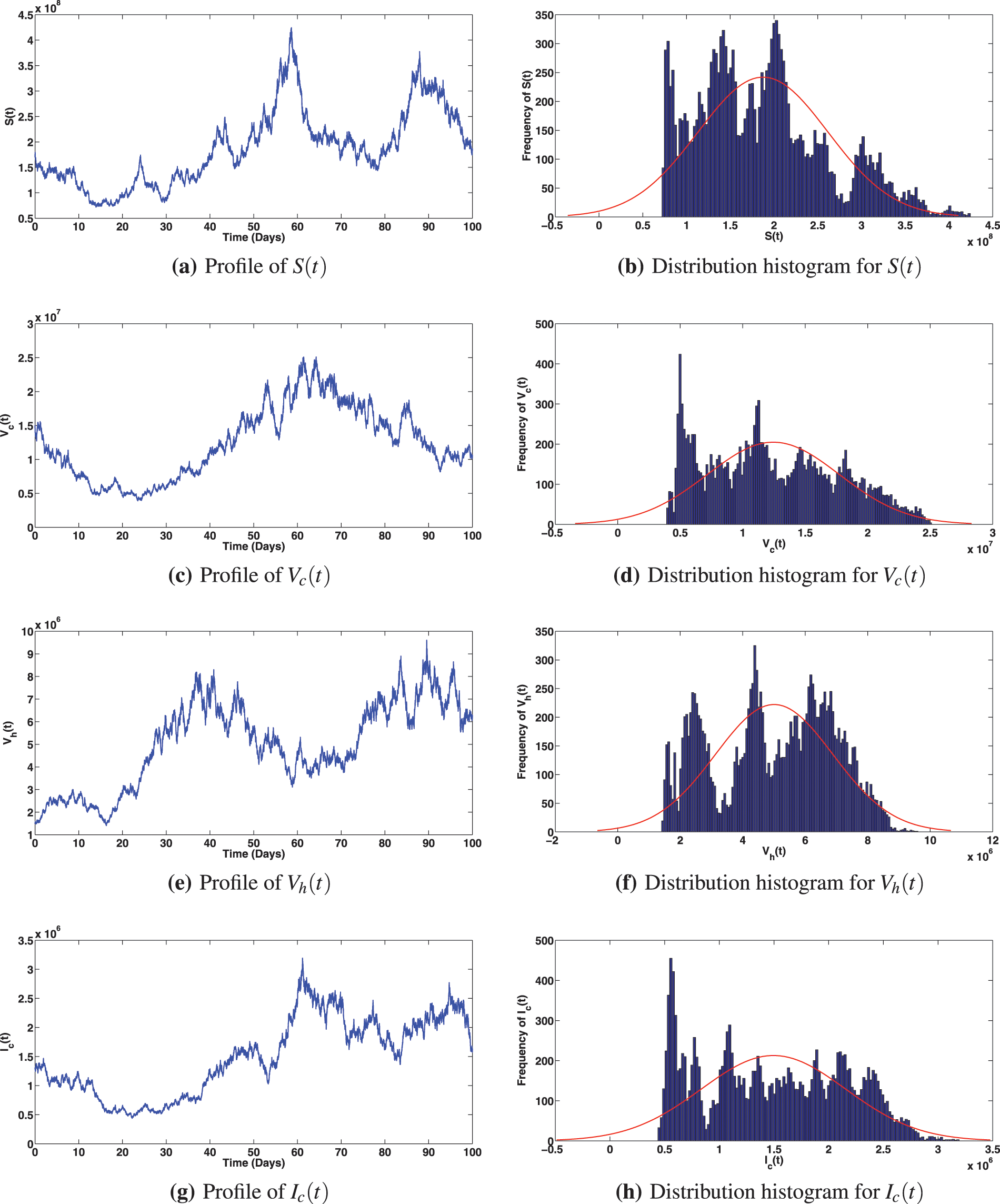
Figure 3: Solution profiles for the various compartments when
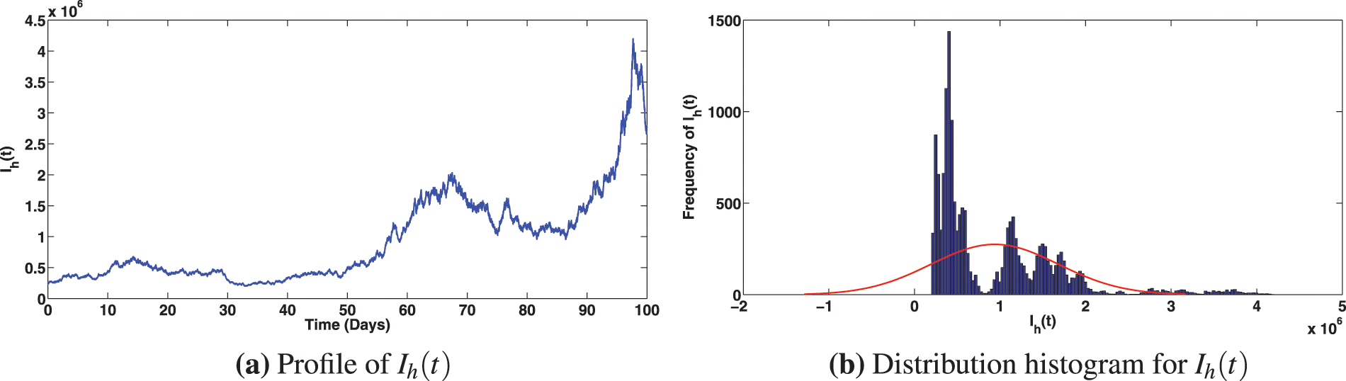
Figure 4: Solution profiles for the various compartments when
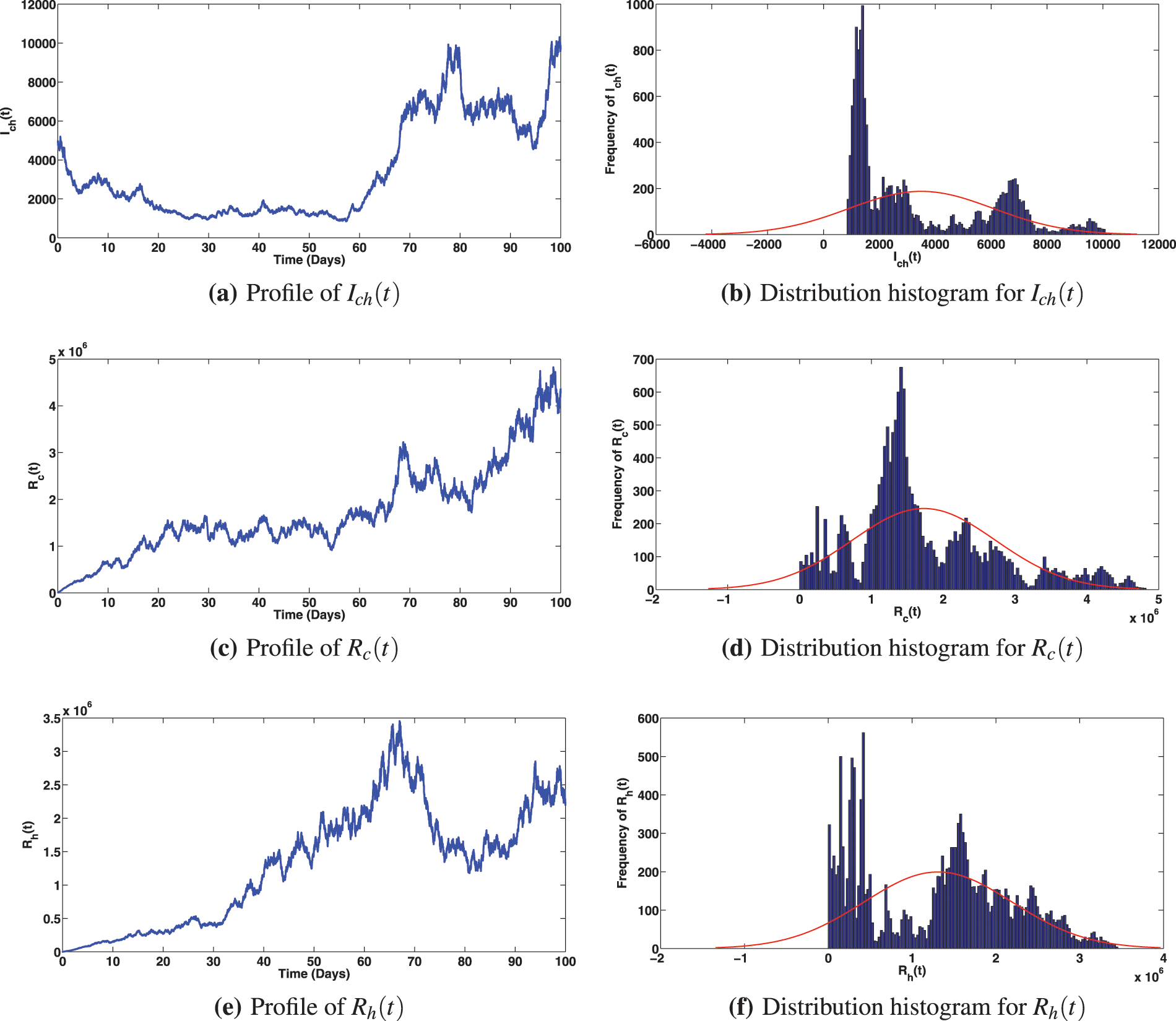
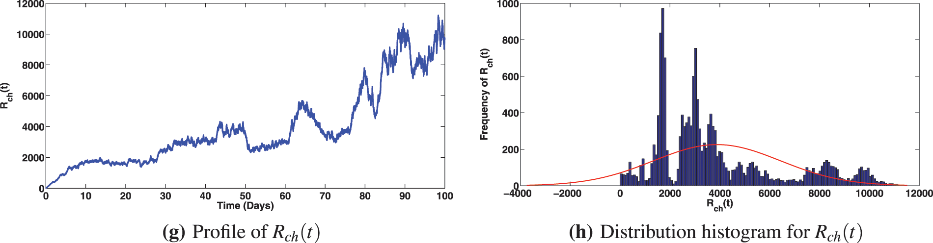
Figure 5: Solution profiles for the various compartments when
5.1 Impact of Primary and Booster Vaccination Rates
Numerical assessments of the epidemiological impact of COVID-19 and viral hepatitis B vaccination strategies are presented in Figs. 6 and 7, respectively. The solution profiles for infected components at different primary and booster vaccination rates for COVID-19 are shown in Fig. 6. It is observed that increasing primary and booster dose vaccination rates greatly caused reduction in infected classes with COVID-19 (Fig. 6a as expected). This measure also brought about reduction in the infected individuals with viral hepatitis B and the compartment co-infected with both diseases (as can be noted in Figs. 6b and 6c). It is interesting to observe that, stepping up the COVID-19 primary vaccination rate to,
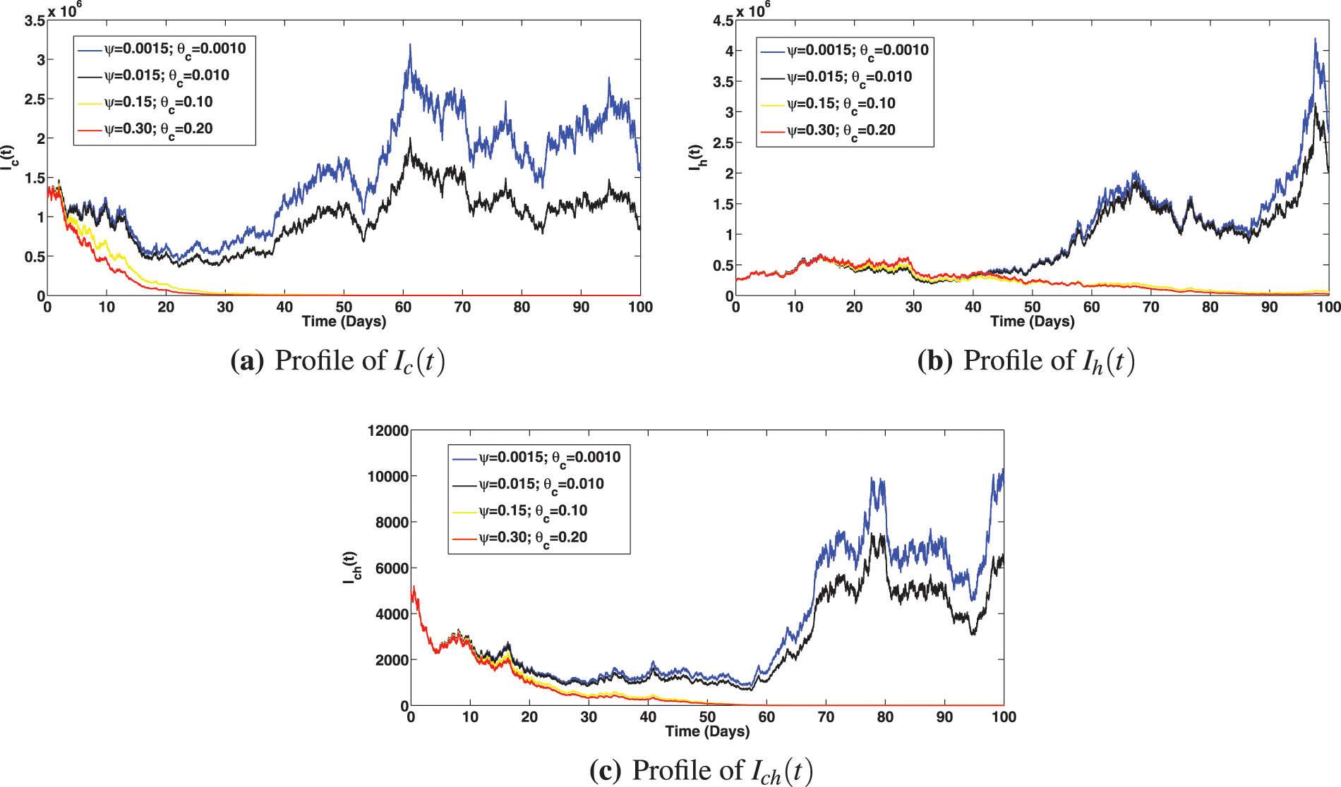
Figure 6: Solution profiles for the infected compartments at different primary and booster vaccination rates for COVID-19, where
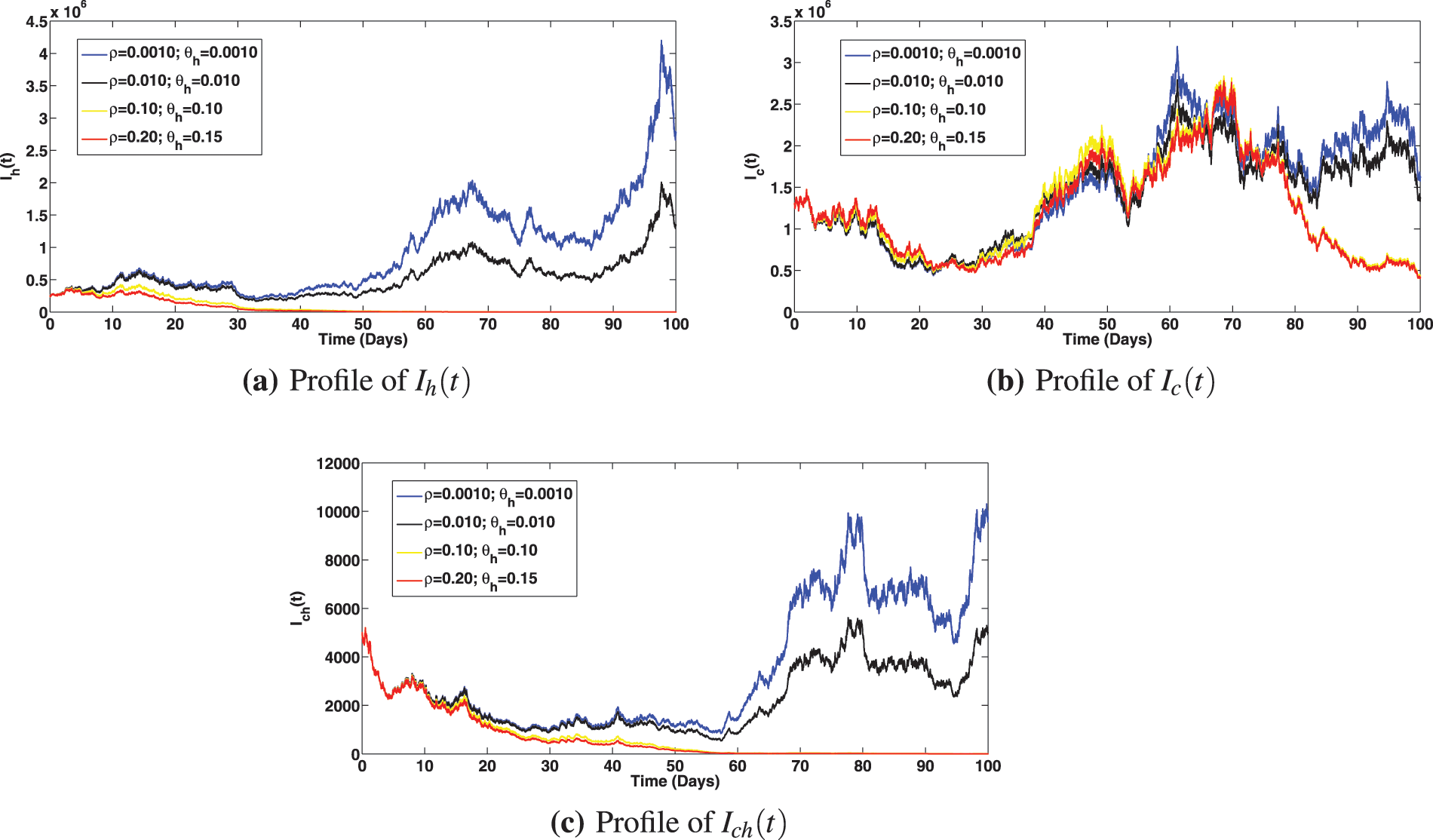
Figure 7: Solution profiles for the infected compartments at different primary and booster vaccination rates for viral hepatitis, where
5.2 Impact of Saturation Effects
The numerical investigation of the epidemiological impact of saturation effect
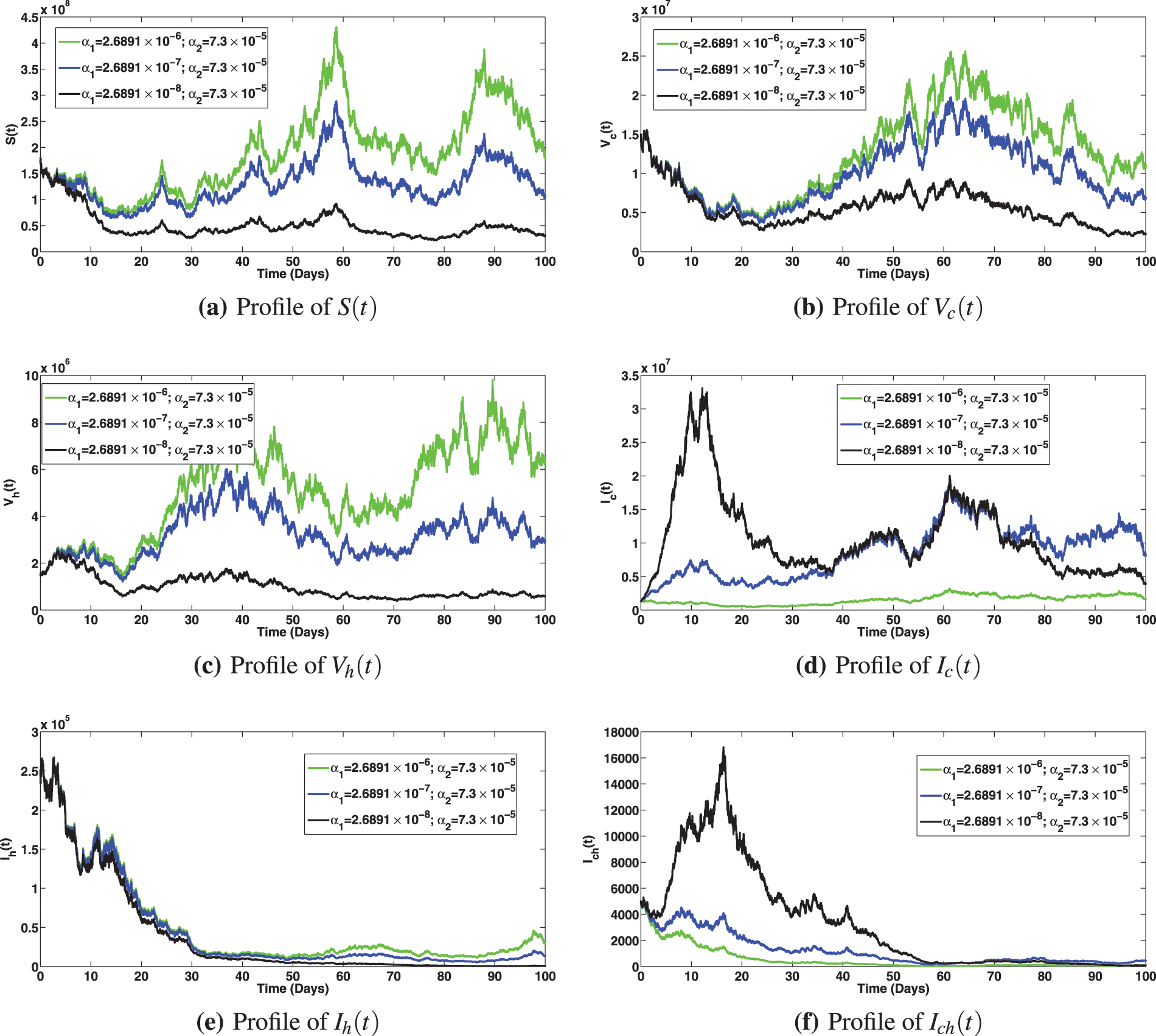
Figure 8: Solution profiles for the various compartments at different saturation effect,
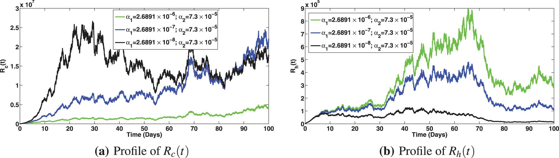
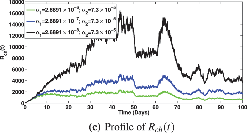
Figure 9: Solution profiles for the various compartments at different saturation effect,
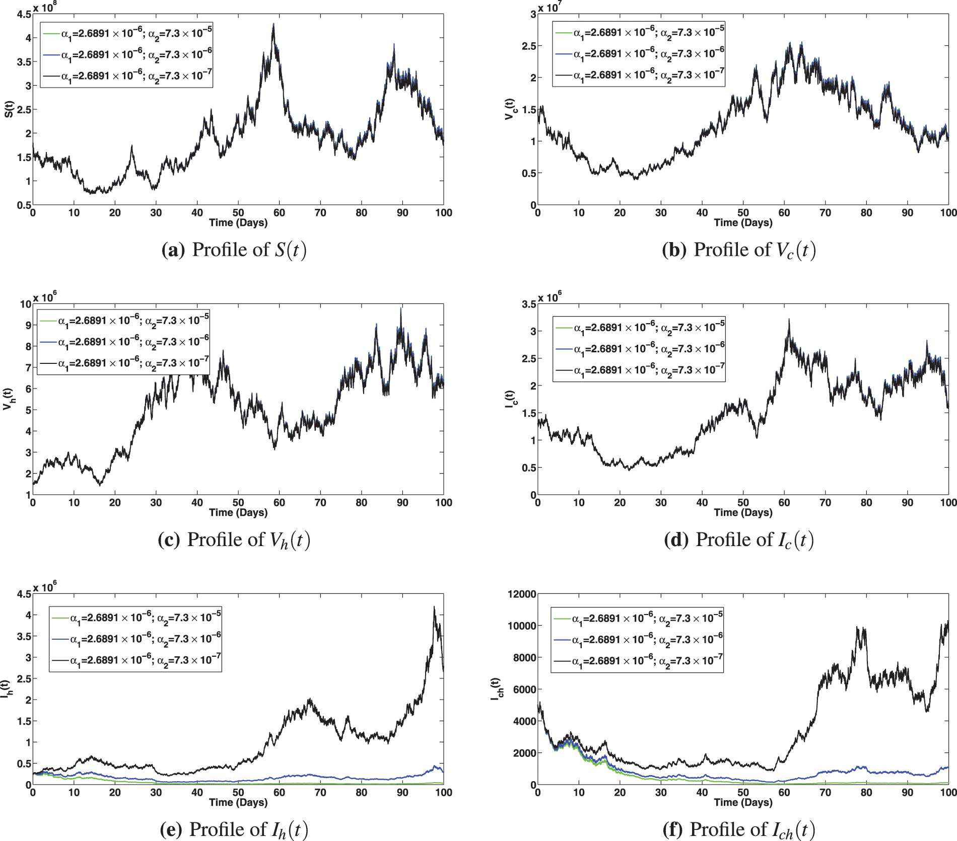
Figure 10: Solution profiles for the various compartments at different saturation effect,
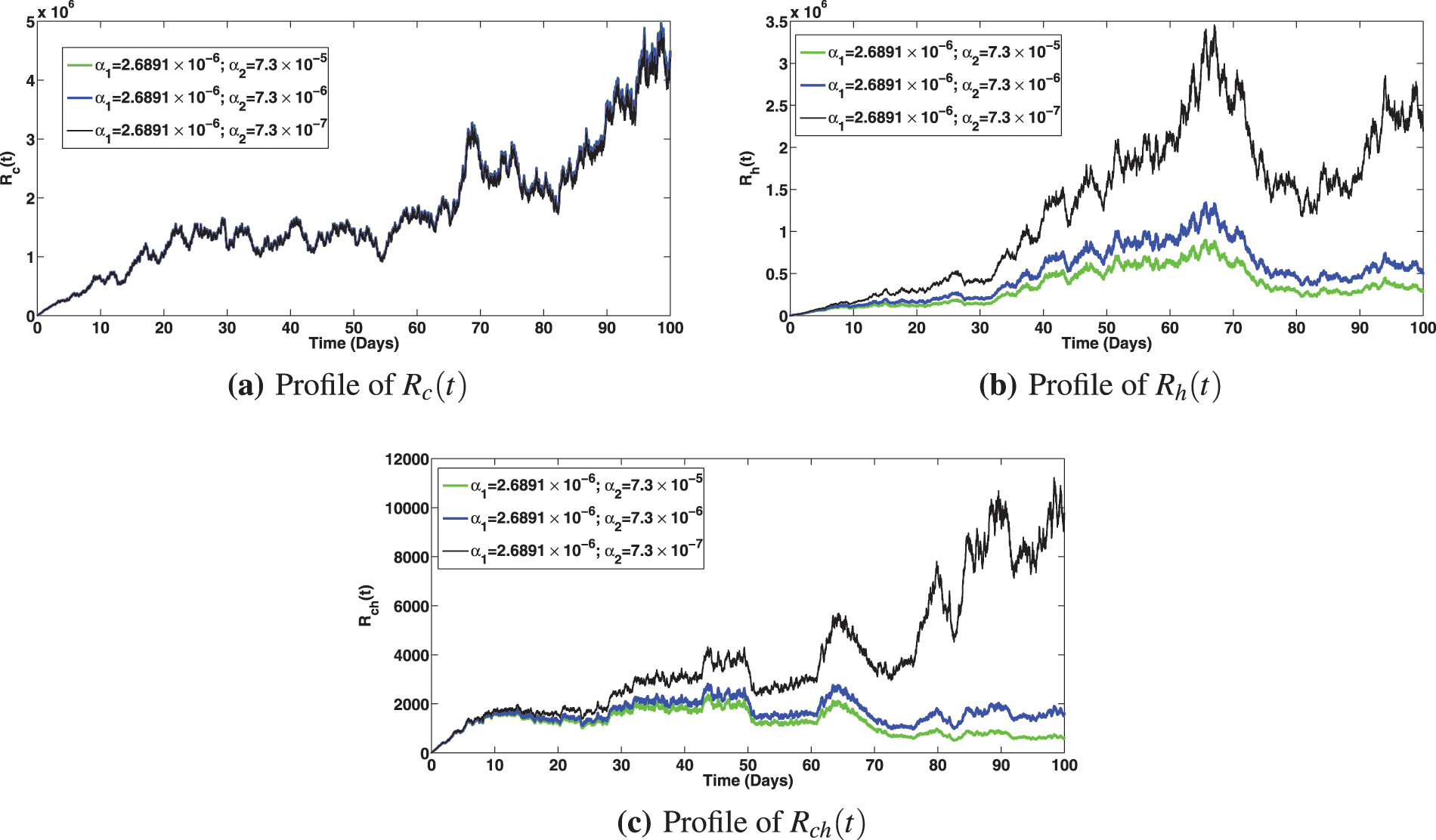
Figure 11: Solution profiles for the various compartments at different saturation effect,
In this paper, a comprehensive stochastic model was developed to assess the epidemiological effect of vaccine booster doses on the co-dynamics of viral hepatitis B and COVID-19 using the real data from Pakistan. The proposed model incorporates logistic growth and saturated incidence functions. Rigorous analyses employing the tools of stochastic calculus have been carried out to find appropriate conditions required for the existence of unique global solutions, stationary distribution in the sense of ergodicity and disease extinction. The stochastic threshold estimated from the data fitting is given by:
(i) The perturbed system was fitted to the real COVID-19 data from Pakistan (depicted by Fig. 2) with stochastic threshold estimated at
(ii) Increasing the COVID-19 primary vaccination rate to
(iii) It is noted from the experiments that increasing primary and booster dose vaccination rates for viral hepatitis B not only caused reduction in infected classes with viral hepatitis B (as seen in Fig. 7a, which is expected) but also brought about a noticeable reduction in the infected individuals with COVID-19 and the co-infection of both diseases (as can be seen in Figs. 7b and 7c).
However, further investigations to improve the present study with fewer limitations can lead to some new avenues of research. More efficient algorithms can be developed for the proposed model with some more realistic assumptions. The model can also consider time dependent contact rates and time delay. Asymptomatic classes can also be considered for both viruses, and data for both diseases to be used for more accurate model fittings. In the future, we shall consider the impact of quadratic Levy noise and variable diffusion rates on the dynamics of both diseases [57–59].
Acknowledgement: The authors wish to express their appreciation to the reviewers for their helpful suggestions which greatly improved the presentation of this paper.
Funding Statement: The authors received no specific funding for this study.
Author Contributions: The authors confirm contribution to the paper as follows: study conception and design: A. O., M. A., D. B.; data collection: A. O., M. A., D. B.; analysis and interpretation of results: A. O., M. A., D. B.; draft manuscript preparation: A. O., M. A., D. B. All authors reviewed the results and approved the final version of the manuscript.
Availability of Data and Materials: All data used for the fitting of the model are available at “Pakistan: Coronavirus Pandemic Country Profile. Available online: https://ourworldindata.org/coronavirus/country/pakistan (accessed on 19/02/2023)”.
Conflicts of Interest: The authors declare that they have no conflicts of interest to report regarding the present study.
References
1. Johns Hopkins Coronavirus Resource Center. https://coronavirus.jhu.edu/map.html (accessed on 24/04/2023) [Google Scholar]
2. Wang, S., Tao, Y., Tao, Y., Jiang, J., Yan, L. et al. (2018). Epidemiological study of hepatitis B and hepatitis C infections in Northeastern China and the beneficial effect of the vaccination strategy for hepatitis B: A cross-sectional study. BMC-Biomedical Central Public Health, 18(3), 1088. https://doi.org/10.1186/s12889-018-5984-6 [Google Scholar] [PubMed] [CrossRef]
3. Centers for Disease Control and Prevention, About Global Hepatitis B. https://www.cdc.gov/globalhealth/immunization/diseases/hepatitis-b/about/index.html (accessed on 25/01/2023) [Google Scholar]
4. Vos, T., Flaxman, A. D., Naghavi, M., Lozano, R., Michaud, C. et al. (2012). Years lived with disability (YLDs) for 1160 sequelae of 289 diseases and injuries 1990–2010: A systematic analysis for the global burden of disease study 2010. Lancet, 380(9859), 2163–2196. [Google Scholar] [PubMed]
5. Lozano, R., Naghavi, M., Foreman, K., Lim, S., Shibuya, K. et al. (2012). Global and regional mortality from 235 causes of death for 20 age groups in 1990 and 2010: A systematic analysis for the global burden of disease study 2010. Lancet, 380(9859), 2095–2128. [Google Scholar] [PubMed]
6. Liang, X., Bi, S., Yang, W., Wang, L., Cui, G. et al. (2009). Epidemiological serosurvey of hepatitis B in China–declining HBV prevalence due to hepatitis B vaccination. Vaccine, 27(47), 6550–6557. [Google Scholar] [PubMed]
7. Mokhtari, A. M., Moghadami, M., Seif, M., Mirahmadizadeh, A. (2021). Association of routine hepatitis B vaccination and other effective factors with hepatitis B virus infection: 25 Years since the introduction of national hepatitis B vaccination in Iran. Iranian Journal of Medical Sciences, 46(2), 93–102. https://doi.org/10.30476/ijms.2019.83112.1199 [Google Scholar] [PubMed] [CrossRef]
8. Yousafzai, M. T., Qasim, R., Khalil, R., Kakakhel, M. F., Rehman, S. U. (2014). Hepatitis B vaccination among primary health care workers in Northwest Pakistan. International Journal of Health Sciences, 8(1), 67–76. https://doi.org/10.12816/0006073 [Google Scholar] [PubMed] [CrossRef]
9. Li, Y., Xiao, S. Y. (2020). Hepatic involvement in COVID-19 patients: Pathology, pathogenesis, and clinical implications. Journal of Medical Virology, 92(9), 1491–1494. https://doi.org/10.1002/jmv.25973 [Google Scholar] [PubMed] [CrossRef]
10. Zhang, C., Shi, L., Wang, F. S. (2020). Liver injury in COVID-19: Management and challenges. The Lancet Gastroenterology & Hepatology, 5(5), 428–430. https://doi.org/10.1016/s2468-1253(20)30057-1 [Google Scholar] [PubMed] [CrossRef]
11. McGill COVID-19 vaccine tracker. https://covid19.trackvaccines.org/ (accessed on 25/01/2023) [Google Scholar]
12. Mohammed, I., Nauman, A., Paul, P., Ganesan, S., Chen, K. H. et al. (2022). The efficacy and effectiveness of the COVID-19 vaccines in reducing infection, severity, hospitalization, and mortality: A systematic review. Human Vaccines & Immunotherapeutics, 18(1), 2027160. https://doi.org/10.1080/21645515.2022.2027160 [Google Scholar] [PubMed] [CrossRef]
13. Zhao, H., Zhou, X., Zhou, Y. H. (2020). Hepatitis B vaccine development and implementation. Human Vaccines & Immunotherapeutics, 16(7), 1533–1544. https://doi.org/10.1080/21645515.2020.1732166 [Google Scholar] [PubMed] [CrossRef]
14. Zheng, H., Wang, F. Z., Zhang, G. M., Cui, F. Q., Wu, Z. H. et al. (2015). An economic analysis of adult hepatitis B vaccination in China. Vaccines, 33(48), 6831–6839. https://doi.org/10.1016/j.vaccine.2015.09.011 [Google Scholar] [PubMed] [CrossRef]
15. Din, A., Li, Y., Khan, T., Zaman, G. (2020). Mathematical analysis of spread and control of the novel corona virus (COVID-19) in China. Chaos Solitons & Fractals, 141, 110286. https://doi.org/10.1016/j.chaos.2020.110286 [Google Scholar] [PubMed] [CrossRef]
16. Asamoah, J. K. K., Okyere, E., Abidemi, A., Moore, S. E., Sun, G. Q. et al. (2022). Optimal control and comprehensive cost-effectiveness analysis for COVID-19. Results in Physics, 33, 105177. https://doi.org/10.1016/j.rinp.2022.105177 [Google Scholar] [PubMed] [CrossRef]
17. Addai, E., Zhang, L., Preko, A. K., Asamoah, J. K. K. (2022). Fractional order epidemiological model of SARS-CoV-2 dynamism involving Alzheimer’s disease. Healthcare Analytics, 2, 100114. https://doi.org/10.1016/j.health.2022.100114 [Google Scholar] [PubMed] [CrossRef]
18. Aslefallah, M., Yuzbasi, S., Abbasbandy, S. A. (2023). A numerical investigation based on exponential collocation method for nonlinear SITR model of COVID-19. Computer Modeling in Engineering & Sciences, 136(2), 1687–1706. https://doi.org/10.32604/cmes.2023.025647 [Google Scholar] [CrossRef]
19. Sadek, L., Sadek, O., Alaoui, H. T., Abdo, M. S., Shah, K. et al. (2023). Fractional order modeling of predicting COVID-19 with isolation and vaccination strategies in Morocco. Computer Modeling in Engineering & Science, 136(2), 1931–1950. https://doi.org/10.32604/cmes.2023.025033 [Google Scholar] [CrossRef]
20. Alnahdi, A. S., Jeelani, M. B., Wahash, H. A., Abdulwasaa, M. A. (2023). A detailed mathematical analysis of the vaccination model for COVID-19. Computer Modeling in Engineering & Science, 135(2), 1315–1343. https://doi.org/10.32604/cmes.2022.023694 [Google Scholar] [CrossRef]
21. Iqbal, S., Baleanu, D., Ali, J., Younas, H. M., Riaz, M. B. (2021). Fractional analysis of dynamical novel COVID-19 by semi-analytical technique. Computer Modeling in Engineering & Science, 129(2), 705–727. https://doi.org/10.32604/cmes.2021.015375 [Google Scholar] [CrossRef]
22. Din, A., Li, Y., Khan, F. M., Khan, Z. U., Liu, P. (2022). On analysis of fractional order mathematical model of hepatitis B using Atangana-Baleanu Caputo (ABC) derivative. Fractals, 30(1), 2240017. [Google Scholar]
23. Din, A., Li, Y., Yusuf, A., Ali, A. Y. (2022). Caputo type fractional operator applied to hepatitis B system. Fractals, 30(1), 2240023. [Google Scholar]
24. Din, A., Li, Y., Omame, A. (2022). A stochastic stability analysis of a HBV-COVID-19 co-infection model in resource limitation settings. Waves in Random and Complex Media. https://doi.org/10.1080/17455030.2022.2147598 [Google Scholar] [CrossRef]
25. Omame, A., Abbas, M. (2023). Modeling SARS-CoV-2 and HBV co-dynamics with optimal control. Physica A, 615, 128607. https://doi.org/10.1016/j.physa.2023.128607 [Google Scholar] [PubMed] [CrossRef]
26. Din, A., Amine, S., Allali, A. A. (2023). stochastically perturbed co-infection epidemic model for COVID-19 and hepatitis B virus. Nonlinear Dynamics, 111, 1921–1945. https://doi.org/10.1007/s11071-022-07899-1 [Google Scholar] [PubMed] [CrossRef]
27. Din, A., Khan, A., Baleanu, D. (2020). Stationary distribution and extinction of stochastic coronavirus (COVID-19) epidemic model. Chaos Solitons & Fractals, 139, 110036. https://doi.org/10.1016/j.chaos.2020.110036 [Google Scholar] [PubMed] [CrossRef]
28. Rajasekar, S. P., Pitchaimani, M. (2019). Qualitative analysis of stochastically perturbed SIRS epidemic model with two viruses. Chaos Solitons & Fractals, 207–221. https://doi.org/10.1016/j.chaos.2018.11.023 [Google Scholar] [CrossRef]
29. Okuonghae, D. (2022). Analysis of a stochastic mathematical model for tuberculosis with case detection. International Journal of Dynamics and Control, 10, 734–747. https://doi.org/10.1007/s40435-021-00863-8 [Google Scholar] [CrossRef]
30. Okuonghae, D. (2022). Ergodic stationary distribution and disease eradication in a stochastic SIR model with telegraph noises and Levy jumps. International Journal of Dynamics and Control, 10, 1778–1793. https://doi.org/10.1007/s40435-022-00962-0 [Google Scholar] [CrossRef]
31. Omame, A., Abbas, M. (2023). Din A, global asymptotic stability, extinction and ergodic stationary distribution in a stochastic model for dual variants of SARS-CoV-2. Mathematics and Computers in Simulation, 204, 302–336. https://doi.org/10.1016/j.matcom.2022.08.012 [Google Scholar] [PubMed] [CrossRef]
32. Zhao, Y., Jiang, D. (2014). The threshold of a stochastic SIRS epidemic model with saturated incidence. Applied Mathematics Letters, 34, 90–93. [Google Scholar]
33. Spencer, S. (2008). Stochastic epidemic models for emerging diseases (Ph.D. Thesis). University of Nottingham, UK. [Google Scholar]
34. Truscott, J. E., Gilligan, C. A. (2003). Response of a deterministic epidemiological system to a stochastically varying environment. Proceedings of the National Academy of Sciences, 100, 9067–9072. [Google Scholar]
35. Liu, M., Wang, K. (2013). Dynamics of a two-prey one predator system in random environments. Journal of Nonlinear Science, 23, 751–775. [Google Scholar]
36. Britton, T., Lindenstrand, D. (2010). Epidemic modelling: Aspects where stochastic epidemic models: A survey. Mathematical Biosciences, 222, 109–116. [Google Scholar]
37. van Herwaarden, O. A., Grasman, J. (1995). Stochastic epidemics: Major outbreaks and the duration of the endemic period. Journal of Mathematical Biology, 33, 581–601. [Google Scholar] [PubMed]
38. Allen, L. J. S. (2008). An introduction to stochastic epidemic models. In: Mathematical epidemiology, pp. 81–130. Berlin, Germany: Springer. [Google Scholar]
39. Nasell, I. (2002). Stochastic models of some endemic infections. Mathematical Biosciences, 179, 1–19. [Google Scholar] [PubMed]
40. Rajasekar, S. P., Pitchaimani, M. (2020). Ergodic stationary distribution and extinction of a stochastic SIRS epidemic model with logistic growth and nonlinear incidence. Applied Mathematics and Computation, 377, 125143. https://doi.org/10.1016/j.amc.2020.125143 [Google Scholar] [CrossRef]
41. Omame, A., Abbas, M. (2023). The stability analysis of a co-circulation model for COVID-19, dengue, and zika with nonlinear incidence rates and vaccination strategies. Healthcare Analytics, 3, 100151. https://doi.org/10.1016/j.health.2023.100151 [Google Scholar] [PubMed] [CrossRef]
42. Olaniyi, S. (2018). Dynamics of Zika virus model with nonlinear incidence and optimal control strategies. Applied Mathematics and Information Science, 12(5), 969–982. [Google Scholar]
43. Abidemi, A., Owolabi, K. M., Pindza, E. (2022). Modelling the transmission dynamics of Lassa fever with nonlinear incidence rate and vertical transmission. Physica A: Statistical Mechanics and Its Applications, 597, 127259. https://doi.org/10.1016/j.physa.2022.127259 [Google Scholar] [CrossRef]
44. Opara, C. Z., Uche-Iwe, N., Inyama, S. C., Omame, A. A. (2020). Mathematical model and analysis of an SVEIR model for Streptococcus pneumonia with saturated incidence force of infection. Mathematical Modelling and Applications, 5(1), 16–38. https://doi.org/10.11648/j.mma.20200501.13 [Google Scholar] [CrossRef]
45. Mao, X. (1997). Stochastic differential equations and their applications. Chichester: Horwood. [Google Scholar]
46. Omame, A., Abbas, M., Onyenegecha, C. P. (2022). A fractional order model for the co-interaction of COVID-19 and hepatitis B virus. Results in Physics, 37, 105498. https://doi.org/10.1016/j.rinp.2022.105498 [Google Scholar] [PubMed] [CrossRef]
47. Din, A., Li, Y., Yusuf, A. (2021). Delayed hepatitis B epidemic model with stochastic analysis. Chaos Solitons & Fractals, 146, 110839. [Google Scholar]
48. Omame, A., Okuonghae, D., Nwajeri, U. K., Onyenegecha, C. P. (2022). A fractional-order multi-vaccination model for COVID-19 with non-singular kernel. Alexandria Engineering Journal, 61(8), 6089–6104. https://doi.org/10.1016/j.aej.2021.11.037 [Google Scholar] [CrossRef]
49. Nanduri, S., Pilishvili, T., Derado, G., Soe, M. M., Dollard, P. et al. (2021). Effectiveness of Pfizer-BioNTech and Moderna vaccines in preventing SARS-CoV-2 infection among nursing home residents before and during widespread circulation of the SARS-CoV-2 B.1.617.2 (Delta) variant—National healthcare safety network, March 1-August 1, 2021. Morbidity and Mortality Weekly Report, 70(34), 1163–1166. [Google Scholar] [PubMed]
50. https://www.indexmundi.com/pakistan/demographics_profile.html (accessed on 25/01/2023) [Google Scholar]
51. van den Driessche, P., Watmough, J. (2002). Reproduction numbers and sub-threshold endemic equilibria for compartmental models of disease transmission. Mathematical Biosciences, 180, 29–48. [Google Scholar] [PubMed]
52. Khas’minskii, R. (2012). Stochastic stability of differential equations, stochastic modelling and applied probability 66, 2nd edition. Berlin Heidelberg: Springer-Verlag. https://doi.org/10.1007/978-3-642-23280-0_1 [Google Scholar] [CrossRef]
53. Dynkin, E. B., Fabius, J., Greenberg, V., Maitra, A., Majone, G. (1965). Markov processes. In: Grundlehren der mathematischen Wissenschaften, vol. 121. New York: Academic Press Inc. [Google Scholar]
54. Weir, A. J. (1973). The convergence theorems. In: Lebesgue integration and measure, pp. 93–118. Cambridge: Cambridge University Press. [Google Scholar]
55. Higham, D. (2001). An algorithmic introduction to numerical simulation of stochastic differential equations. Siam Review, 43(3), 525–546. [Google Scholar]
56. Pakistan: Coronavirus Pandemic Country Profile. https://ourworldindata.org/coronavirus/country/pakistan (accessed on 11/01/2023) [Google Scholar]
57. Rajasekar, S. P., Pitchaimani, M., Zhu, Q. (2022). Probing a stochastic epidemic hepatitis C virus model with a chronically infected treated population. Acta Mathematica Scientia, 42, 2087–2112. https://doi.org/10.1007/s10473-022-0521-1 [Google Scholar] [PubMed] [CrossRef]
58. Sabbar, Y., Kiouach, D., Rajasekar, S. P., El-idrissi, S. E. A. (2022). The influence of quadratic Lévy noise on the dynamic of an SIC contagious illness model: New framework, critical comparison and an application to COVID-19 (SARS-CoV-2) case. Chaos, Solitons & Fractals, 159, 112110. https://doi.org/10.1016/j.chaos.2022.112110 [Google Scholar] [PubMed] [CrossRef]
59. Pitchaimani, M., Rajasekar, S. P. (2018). Global analysis of stochastic SIR model with variable diffusion rates. Tamkang Journal of Mathematics, 49(2), 155–182. [Google Scholar]
Cite This Article
 Copyright © 2024 The Author(s). Published by Tech Science Press.
This work is licensed under a Creative Commons Attribution 4.0 International License , which permits unrestricted use, distribution, and reproduction in any medium, provided the original work is properly cited.
 Downloads
 Citation Tools