
 Submit a Paper
 Propose a Special lssue
 Open Access
ARTICLE
Fractional Gradient Descent RBFNN for Active Fault-Tolerant Control of Plant Protection UAVs
1 School of Mechanical Engineering, Yangzhou University, Yangzhou, 225009, China
2 College of Intelligent Manufacturing, Yangzhou Polytechnic Institute, Yangzhou, 225009, China
3 School of Automation, Nanjing University of Aeronautics and Astronautics, Nanjing, 211106, China
* Corresponding Author: Jianfeng Zhang. Email:
Computer Modeling in Engineering & Sciences 2024, 138(3), 2129-2157. https://doi.org/10.32604/cmes.2023.030535
Received 12 April 2023; Accepted 26 July 2023; Issue published 15 December 2023
 View Full Text
 Download PDF
Abstract
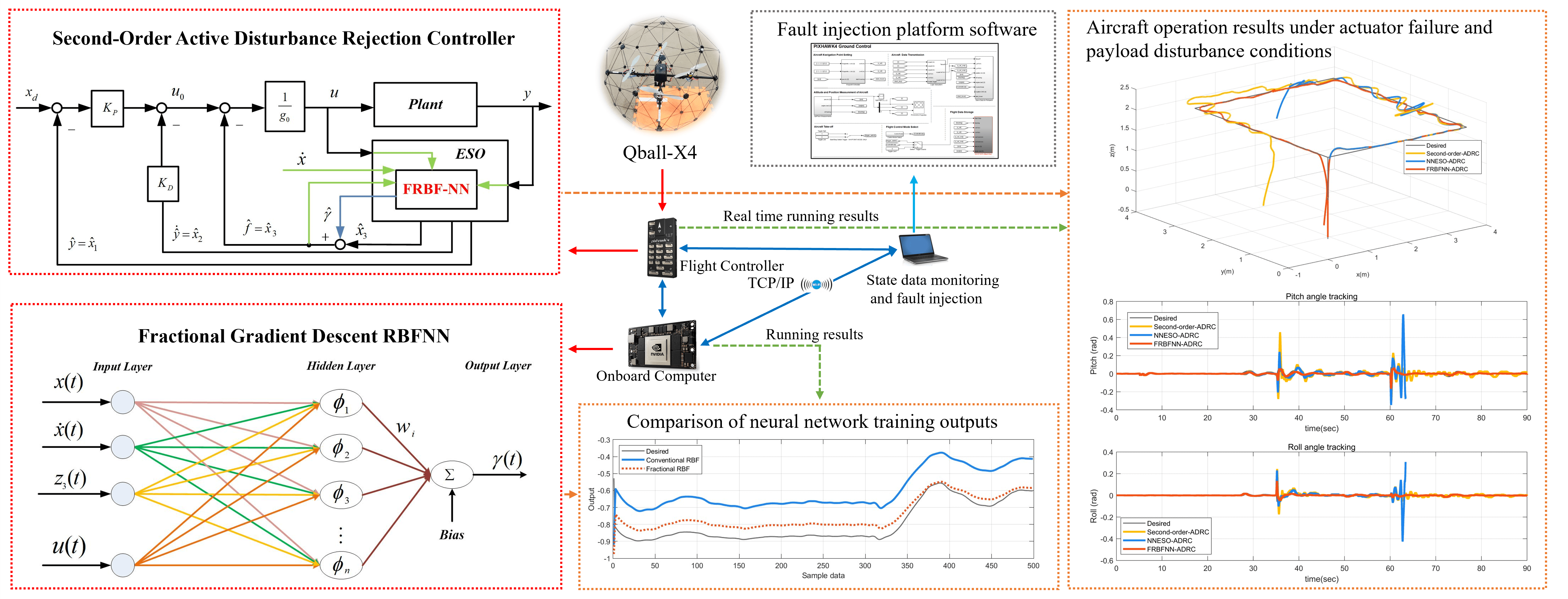
With the increasing prevalence of high-order systems in engineering applications, these systems often exhibit significant disturbances and can be challenging to model accurately. As a result, the active disturbance rejection controller (ADRC) has been widely applied in various fields. However, in controlling plant protection unmanned aerial vehicles (UAVs), which are typically large and subject to significant disturbances, load disturbances and the possibility of multiple actuator faults during pesticide spraying pose significant challenges. To address these issues, this paper proposes a novel fault-tolerant control method that combines a radial basis function neural network (RBFNN) with a second-order ADRC and leverages a fractional gradient descent (FGD) algorithm. We integrate the plant protection UAV model’s uncertain parameters, load disturbance parameters, and actuator fault parameters and utilize the RBFNN for system parameter identification. The resulting ADRC exhibits load disturbance suppression and fault tolerance capabilities, and our proposed active fault-tolerant control law has Lyapunov stability implications. Experimental results obtained using a multi-rotor fault-tolerant test platform demonstrate that the proposed method outperforms other control strategies regarding load disturbance suppression and fault-tolerant performance.Graphic Abstract
Keywords
In the past decade, multi-rotor unmanned aerial vehicle (UAV) technology has developed rapidly and is widely used in various industries, such as national defense, construction, power, rescue, and agriculture [1–5]. Different types of components, such as onboard computers, sensors, cameras, and controllers, are carried by multirotor UAVs to meet the requirements of various mission scenarios. Furthermore, multi-rotor UAVs’ external disturbance rejection capability and fault tolerance also vary according to different scenarios. Therefore, many researchers have studied flight control algorithms for specific types of UAVs and their application scenarios [6–8].
The control system of a multi-rotor UAV is a typical underactuated system with nonlinear characteristics [9,10]. In the control algorithm of multirotor UAVs, the most common methods are the PID control algorithm [11], sliding mode control algorithm [12–14], and robust control algorithms such as disturbance rejection control [6,15,16]. With the increasing complexity of multirotor UAVs [17–20], researchers have considered combining adaptive control technology with robust control technology to better control such complex systems [14]. To address the uncertain dynamic parameters and external disturbances in the system, Lu et al. used neural networks to identify uncertain parameters in the system, which performed well in the control of such nonlinear systems [21]. However, the instability of the control system due to external or self-disturbances, as well as actuator and sensor failures, is a common phenomenon for UAVs [22,23]. Therefore, many researchers have considered combining intelligent control algorithms with robust and adaptive control to propose fault-tolerant control algorithms that can solve a class of faults [24–26]. Boche et al. proposed a fault-tolerant control scheme that utilizes continuous and discrete methods to address multiple actuator failures [27]. Alternatively, Wen et al. proposed an adaptive neural fuzzy sliding mode control method with online parameter updating in reference [28] to solve the fault-tolerant control problem of uncertain nonlinear systems subjected to actuator effectiveness failures and input saturation, regardless of fault limits. However, in some fault-tolerant control methods, the fuzzy neural network structure remains fixed and cannot independently adjust the fuzzy rule number, leading to increased computational burden and potential negative impacts on control performance when inputs and outputs increase. To address this issue, Yu et al. proposed an actuator fault-tolerant control method that utilizes a self-constructed fuzzy neural network and multivariable sliding mode control [23]. By combining adaptive algorithms with self-constructed fuzzy neural networks, the proposed method approximates actuator fault information and model uncertainty parameters, thus reducing the computational burden of the control system and ensuring stable fault systems within a finite time. Moreover, radial basis functions offer significant advantages in dealing with parameter approximation of nonlinear systems. Similarly, Xiang et al. used an observer combined with RBFNN to detect unknown faults in the system with changing model dynamics in the attitude system of the aircraft. Because of the advantages of neural networks in function approximation and data classification processing, they can handle model uncertainty changes and distinguish fault data in the case of actuator failures [29]. However, the fault-tolerant control method implemented has certain requirements for the construction of the system model. Therefore, it is necessary to find a control algorithm that does not overly rely on the system model. Zhou et al. proposed a fault-tolerant control method combining self-disturbance control and a radial basis function neural network to give the system a certain fault-tolerant control ability for actuator and sensor failures while resisting external disturbances [15]. The active disturbance rejection control algorithm has the characteristic of not overly relying on the system model, and is a good solution for control systems with uncertain models. However, for systems where changes in system model parameters are detected, using machine learning algorithms is also a good solution [30]. Zhong et al. introduced the model reference adaptive control into the RBFNN for online identification of the system model’s changing parameters [16]. Similarly, Liu et al. designed a new cascade double loop ADRC method of neural network-based extended state observer (NNESO) to solve the attitude control problem of hypersonic vehicles in order to solve the disturbance problem of hypersonic vehicles [22]. The controller design ideas in this article have given us some inspiration. To better identify the uncertain items of dynamic parameters of systems, Hua et al. used optimized parameters of a self-disturbance control algorithm and combined them with a spatiotemporal RBFNN to achieve fault-tolerant control for actuator failures in a class of nonlinear systems, and significant results were obtained [31]. This article further studies on this basis.
However, the above research needs further investigation into the disturbance and fault-tolerant control algorithms for plant protection UAVs under heavy loads. Moreover, with the rapid development and application of plant protection UAVs, research on safety control mechanisms for this type of UAV has become increasingly important [32]. For this reason, the disturbance problem of UAV attitude control caused by loads in various load situations has received attention from many researchers [33]. Guerrero-Sanchez et al. proposed a hybrid control method combining a feedback linearization controller and artificial neural network for a UAV’s suspended load situation, using the artificial neural network as an estimator of load disturbance to achieve disturbance control of the UAV under the load situation [34]. Similarly, Ameya et al. proposed a self-attenuation control strategy based on an extended state observer for effective payload mathematical modeling of UAVs. The approach considers the payload as an external disturbance of the system, employs the extended state observer to estimate the disturbance term, and then designs a self-attenuation controller to achieve stable control of the UAV [8].
In summary, plant protection UAVs are prone to actuator failures and must carry a significant amount of pesticide, thus requiring solutions for disturbance suppression and fault-tolerant control. To effectively control the UAV while carrying pesticides, we build upon the second-order ADRC developed by Herbst [35] and design an extended state observer (ESO). Additionally, to achieve fault-tolerant flight control during actuator failure, we propose a novel approach combining a radial basis function neural network (RBFNN) with a fractional-order gradient descent algorithm-based extended state observer to identify system generalized parameter terms [36]. This method utilizes a convex combination of the traditional RBFNN and a fractional gradient descent method with improved Riemann-Liouville derivatives, resulting in better nonlinear system identification capabilities than traditional RBFNN. We compared and analyzed the proposed fault-tolerant controller with traditional RBFNN and NNESO based ADRC controllers to evaluate the performance of fault-tolerant flight control. Through simulations, we have observed that the proposed method exhibits smaller overshoots for limited actuator gain and bias failures and efficiently suppresses oscillations caused by load disturbances. Our research contributions can be summarized as follows:
1. A second-order ADRC was designed to estimate nonlinear systems’ uncertain parameters and load disturbances, which can suppress load disturbances and the impact of uncertain system modeling parameters with minimal parameter adjustment. The experimental results showed that this method could better suppress load disturbances and faster response speed.
2. An optimized extension state observer was proposed based on the second-order ADRC and a novel RBFNN with a fractional gradient descent algorithm with the optimal system identification solution. The output of the gradient descent RBFNN was combined with the high-order parameter estimation part of the ADRC observer to enhance the UAV’s ability in disturbance suppression and reduce the error between the aircraft’s attitude control angle and the desired angle.
3. The actuator’s bias and gain fault items were integrated into the general parameter term, and the number of design parameters for the adaptive control was optimized. Flight state data of a plant protection UAV with actuator faults and loads were collected for model training of the gradient descent RBFNN, enabling the ADRC to have anti-disturbance and fault-tolerant control capabilities for the UAV in the presence of actuator faults and disturbances.
This article describes an independent fault-tolerant flight control design for a quadrotor aircraft’s pitch, roll, and yaw subsystems. The proposed approach utilizes the aircraft’s attitude angles and angular velocities to train weight parameters of a fractional-order RBFNN, which can better approximate the values of the fused parameter terms in the presence of modeling error, uncertainty, disturbance, and fault. Moreover, the proposed fault-tolerant flight control scheme can simultaneously handle multiple limited faults in the actuators. The stability of the designed control law is proven using Lyapunov stability analysis. Finally, simulation experiments are conducted on a fault injection platform for plant protection UAVs to demonstrate the excellent performance of the proposed algorithm.
The rest of this paper is organized as follows. Section 2 presents the aerodynamic model of the plant protection UAV, including the load model and actuator fault model. Section 3 introduces the design of a second-order ADRC with a generalized observer and an RBFNN based on the FGD learning algorithm. In Section 4, a second-order ADRC fault-tolerant controller with Lyapunov stability is designed based on the backstepping control approach. Section 5 describes the fault injection simulation experiments conducted on the Qball-X4 UAV using the modified model parameters that match the plant protection UAV and evaluates the performance of the designed fault-tolerant controller. Finally, Section 6 summarizes the work presented in this paper and discusses potential future research directions.
2 Mathematical Model of X-Type Quadrotor UAV
This section introduces the dynamic model of a quadrotor aircraft carrying a pesticide load. The aircraft’s center of mass changes continuously during the flight due to the absence of a fixed form of pesticides and other spraying liquids in the water tank of the plant protection UAV. To simplify the analysis of the dynamic model of the quadrotor aircraft, we make the following assumptions:
1. The centroid of the water tank body remains unchanged.
2. Approximating a pesticide liquid in an aqueous phase as a particle.
3. Neglecting aerodynamic effects on aircraft and mounted water tanks.
4. Water tank and aircraft as a completely rigid structure.
To develop an effective control algorithm for quadrotor aircraft, it is imperative to obtain accurate state information regarding the aircraft’s angular orientation, angular acceleration, linear velocity, and linear acceleration. As such, this section provides a brief analysis of the interrelationship between the airframe coordinate system and the inertial coordinate system of the quadrotor UAV, as well as an examination of the mathematical expressions of the parameters pertinent to quadrotor dynamics.
The dynamics model of a quadrotor aircraft has been proposed in many papers on quadrotor aircraft control [9,10]. To obtain the mathematical model of the plant protection UAV with a liquid load, we present in Fig. 1 the kinematic parameters of a quadrotor aircraft with a liquid load in a water tank.
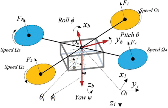
Figure 1: Quadrotor plant protection UAV
Moreover, we established the body coordinate system
where
where
In theory, a rigid multi-rotor aircraft can maintain its attitude stability by ensuring that each rotor provides equal thrust. Additionally, adjusting the thrust of the four rotors can change the position and attitude of the aircraft. Hence, based on the system dynamics model presented in Eqs. (2) and (3), the controller design can be carried out for the following affine nonlinear system:
Among them, the state variables
2.2.1 Model of Load Liquid Disturbance
Load disturbance can have a significant impact on UAV control during task execution. To mitigate this effect, various control methods have been proposed by researchers [8,34]. Similarly, the shaking of the aircraft water tank can cause interference with the stability of the aircraft’s attitude. As shown in Fig. 2, the relative static model of the UAV on the x-axis plane at a certain moment during the movement of the liquid in the water tank can be observed.
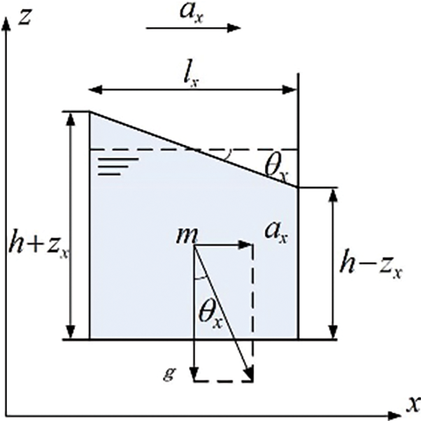
Figure 2: Static liquid model at the equilibrium moment
Fig. 2 illustrates parameters related to the systematic motion of liquid on the OXZ coordinate plane. Here, the UAV is assumed to move with a constant acceleration at (m/s2), while the liquid system exhibits acceleration components along the x-axes and y-axes, denoted by ax and ay, respectively. The distances between the UAV’s axis and the liquid’s virtual centers of mass along the x-axes and y-axes are denoted by lx and ly, respectively. Here h is the distance (height) between the liquid level in the tank and the tank bottom at the initial time, g is gravity acceleration,
At the initial moment, the forces of liquid formation in the x-axes and y-axes directions are derived as:
where
Then, the forces exerted by the liquid along the
At the moment of equilibrium, the force along the x and y-axes is the sum of the force exerted on the swaying part and the force exerted on the relatively stationary part:
At the moment of balance during the movement of the UAV, the force on the water tank along the
Assuming that the acceleration of the liquid at the moment of equilibrium is equivalent to that of the drone, the force exerted by the shaking component can be expressed as follows when the liquid system in the tank reaches equilibrium:
The maximum force components of the entire water tank along the x-axes and y-axes can be derived as follows:
The impact of the liquid in the tank on the rigid structure of the aircraft can be quantified by the displacement of the liquid’s center of mass within the container. This displacement is denoted as the movement distance
Accordingly, the disturbance force magnitude that affects the aircraft in the pitch and roll attitude directions due to the liquid in the tank can be calculated as follows:
The disturbance parameters for pitch and roll attitudes can be defined as follows:
In general, in the absence of external disturbances, the lift of a multi-rotor aircraft is provided by the lift generated by each propeller, and the lift
where
However, it is difficult to directly obtain the change data of the nonlinear term and actuator fault expressed in the mathematical model in the actual system. Therefore, to simplify the modeling process and facilitate the parameter estimation of the observer designed later. For the convenience of mathematical expression, the following text will ignore the expression form of the independent variable of time. According to Eqs. (1) and (4), the control quantity
where
Here,
In the above equation,
The state space representation of a second-order system model of the UAV given in Eq. (16) can be expressed as follows:
In Eq. (16), the fault and disturbance parameter terms in the system are quite complex. If an RBFNN is used to identify each parameter part, it will complicate the observer design and increase the computation of the controller. Therefore, for the convenience of the subsequent design of the ADRC observer, we further optimize and introduce a generalized disturbance term f. The second-order attitude model of the system in the state-space model can be expressed as:
Here, the generalized disturbance term f actually contains system state parameters, load disturbance
The basic idea in the design process of an active disturbance rejection controller (ADRC) is to develop an extended state observer (ESO) capable of estimating both the system state and total disturbance. The generalized disturbance term has been defined in Eq. (19). To estimate the generalized disturbance term f, it is considered as the extended state
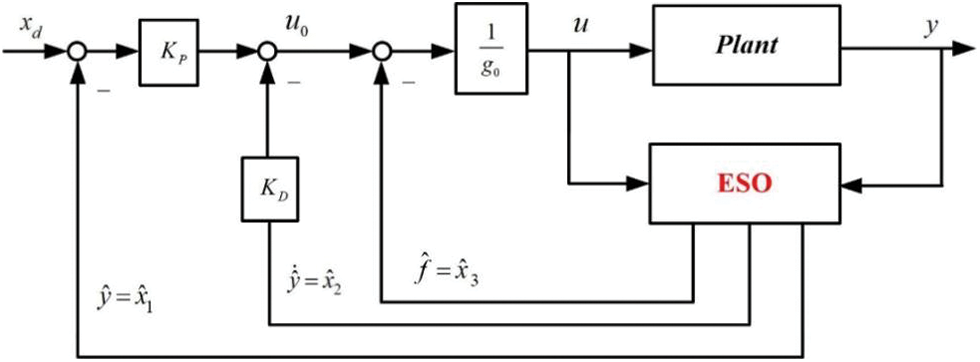
Figure 3: ADRC ring structure for second-order processes
The linear controller can achieve disturbance suppression and integral chain behavior by using estimation variables, and the extended state observer of the system can be obtained as follows:
where
As mentioned above, we have implemented a residual double integral behavior with disturbance suppression and a linear controller. Then, we can obtain a controller based on extended state feedback.
Therefore, according to the second-order ADRC structure designed in Fig. 3,
where
Replacing the above equation in (18), the second-order system model can be expressed as
In general, the closed loop can be adjusted to the critically damped state with
Typically, for any second-order dynamic system, a PD controller can be used to adjust the closed loop to the critical damping state, and for the desired 2% settling time T, a negative real pole can be obtained by selecting proportional parameter
The placement of the poles of the ESO can be determined empirically and typically take the following values:
After the pole positions are thus selected, the observer gain is calculated according to the characteristic polynomial of the matrix (
Then, the solution for
In summary, the control law of the ADRC controller for a class of nonlinear second-order systems can be designed as follows:
3.2 Design of the ADRC Expanded State Observer Based on a Neural Network
The effectiveness of the attitude controller is crucial for the flight performance of plant protection unmanned aerial vehicles, especially in the presence of possible actuator faults. However, the control law proposed in this paper, which incorporates an estimate of the generalized disturbance term, can only achieve stable attitude control when the drone has a small degree of fault, as discussed in the experimental section. When the UAV (drone) has a large load, the proposed control law cannot achieve stable attitude control. Therefore, further research is needed to develop more robust control laws to handle larger disturbances and actuator faults. This article further improves on the previously designed fault-tolerant controller [31]. Therefore, this paper proposes a novel approach to estimate the generalized disturbance term in identifying a class of second-order nonlinear systems called the fractional gradient descent (FGD) learning algorithm. The proposed algorithm is illustrated in Fig. 4, which is incorporated into an ADRC controller structure.
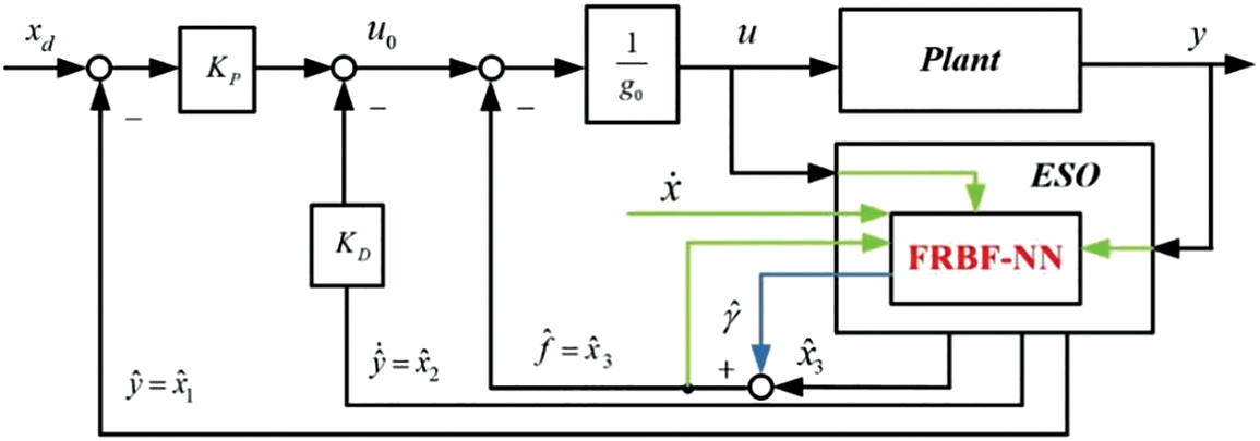
Figure 4: ADRC controller based on FRBF-NN
The experimental results demonstrate that the proposed method is effective in convergence and steady-state performance compared to the classical RBF neural network. The FRBF-NN proposed in this paper is a mathematical variant of the classical RBF-NN, and an algorithmic improvement is proposed in the intrinsic concept of gradient descent optimization.
The structural diagram of the proposed RBFNN is presented in Fig. 5.
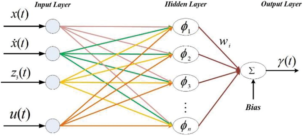
Figure 5: The FRBF-NN structural diagram
The RBF network structure consists of three layers: the input layer, the nonlinear hidden layer, and the linear output layer, as shown in Fig. 5. If we consider the input vector as
In the RBFNN structure shown in Fig. 5, m represents the number of hidden layer neurons,
where
where
where
The weight updating equation of the gradient descent method with a mixed parameter q and a fractional gradient term is given as follows:
The parameters in this equation include
We use the chain rule to compute the factors
Similarly, the fractional derivative of ladder
By simplifying the two formulas above, we obtain
Then, formula
To simplify the computation, we consider
The update rule for
4 Design of Fault-Tolerant Controller and Proof of Stability
In a multi-rotor control system, the control output for the pitch and roll attitude of the aircraft exceeds its input, making it a typical underactuated system. In the event of a failure, the stability of the attitude system becomes paramount. Therefore, this section primarily focuses on designing the controller for the aircraft’s attitude system.
First, based on the affine nonlinear system given in Eq. (16), we define
where
To achieve stable control over
The derivative of time with respect to that is:
From Eq. (43),
Therefore, the error variable can be defined by introducing the virtual control quantity
Then, the Eq. (46) can be expressed as:
Therefore, when the virtual control quantity
Then, based on the expression of Eq. (45), the time derivative of
Then, according to Eq. (43), it is further derived
However, to satisfy the Lyapunov function’s stability condition
Then,
Therefore, if
Taking the derivative of the latter yields
To satisfy the Lyapunov function’s stability condition
Among them,
Finally, the control that makes the system asymptotically stable can be inversely solved
A multirotor UAV itself is a high-order system, and the introduction of higher-order variables can increase system instability. Therefore,
We can obtain the fault-tolerant control law in which the higher-order variables are omitted:
Furthermore, the final form of the Lyapunov function can be determined based on Eqs. (45) and (54):
Next, we take the derivative of the above function:
It is easy to see that if
Similarly, the derivative of the Lyapunov function
5 Simulation Results and Analysis
This section aims to compare the effectiveness of the proposed fault-tolerant control algorithm with traditional methods through flight experiments and simulation experiments, specifically on the Qball-X4 unmanned aerial vehicle (UAV) model.
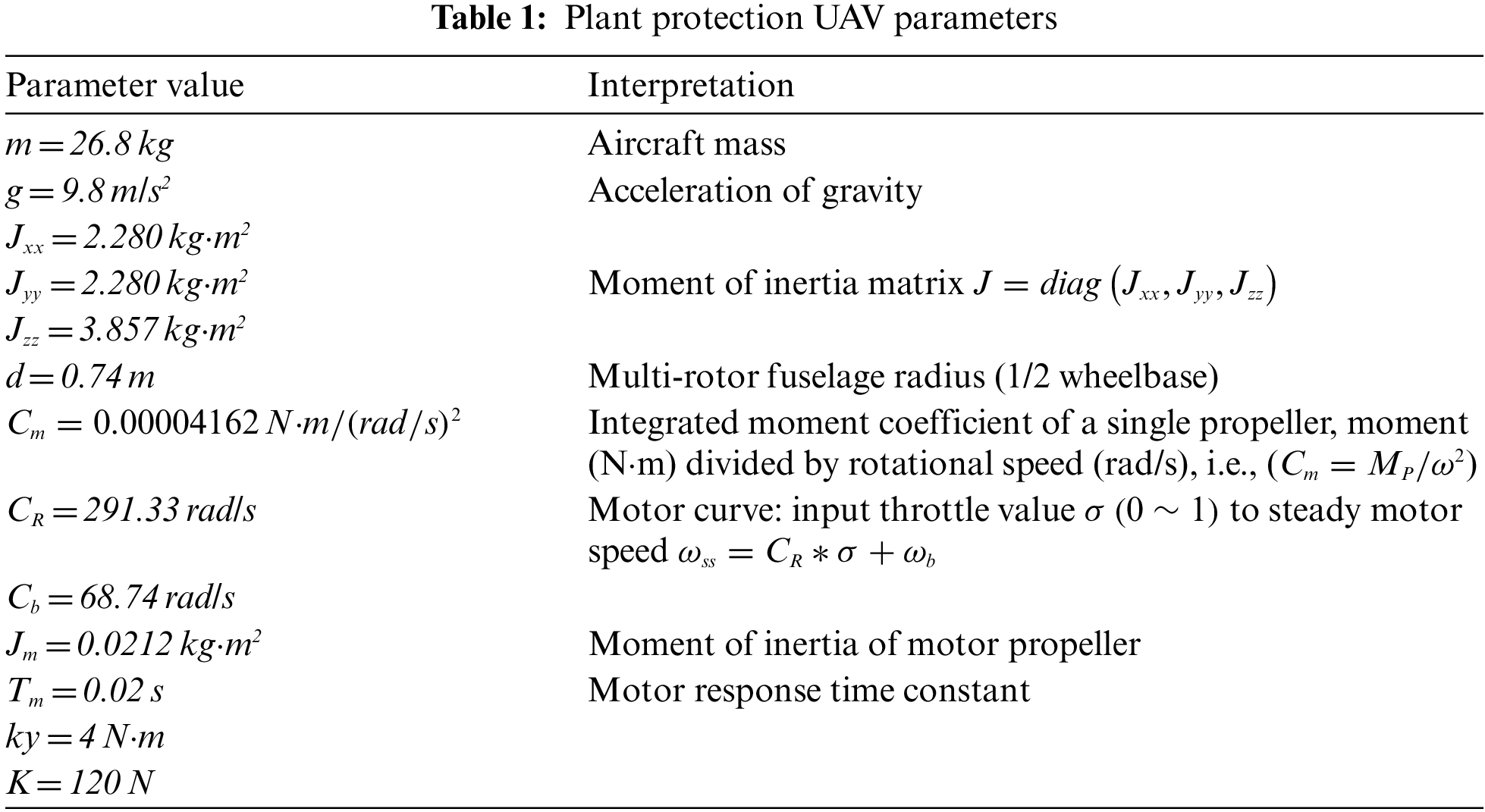
Real-time control and monitoring during the experiment were accomplished through the TCP/IP communication protocol between the onboard computer and the computer-based ground station. The numerical values of the initial model parameters for the modified crop-spraying drone are shown in Table 1.
As shown in Fig. 6, the fault injection system of the Qball-X4 UAV model used PIXHAWK4 as the UAV flight control unit, and the Jetson TX2 onboard computer served as the data acquisition and calculation unit for the neural network estimator.
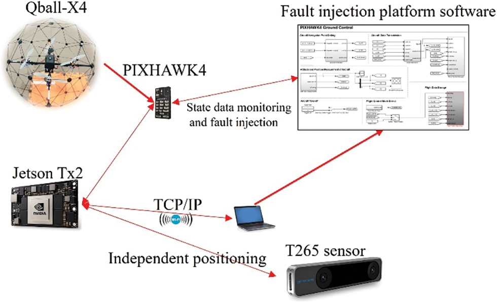
Figure 6: Qball-X4 quadrotor UAV fault injection system
To effectively analyze the control performance of the proposed ADRC (RBFNN) fault-tolerant flight control algorithm, we collected system state data of the Qball-X4 UAV during actual flight, including the state matrix
First, in the training process of the proposed gradient descent-based radial basis function neural network (FRBFNN) in this paper, to improve the fitting and accuracy of FRBFNN output parameter estimation with real data, flight state data of the aircraft were collected under normal, payload, and fault conditions.
We used the attitude state parameter
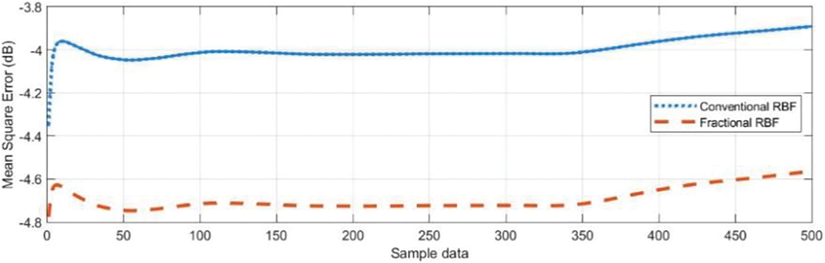
Figure 7: MSE testing curves
Figs. 8 and 9 show that the FRBF-NN has a more accurate tracking and prediction effect on the sample data than the traditional RBFNN, with slightly smaller tracking errors and error values tending toward zero.
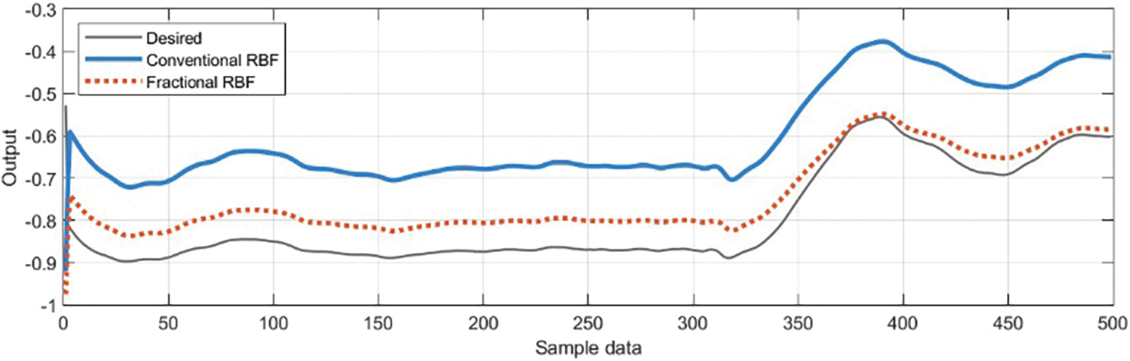
Figure 8: Predicted results of the FRBF-NN and traditional RBFNN
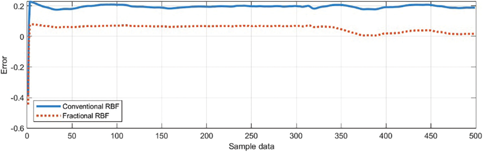
Figure 9: The prediction errors of the FRBF-NN and traditional RBFNN
In summary, we have developed an offline FRBF-NN model for plant protection UAVs with load disturbances and actuator faults, which provides a faster and more accurate estimation of fault and disturbance parameters than traditional RBFNN models. To further verify and compare the effectiveness and advantages of the proposed fault-tolerant control algorithm, we designed the following simulation scenarios to evaluate the controller’s performance:
Scenario 1: An agricultural drone with a load disturbance of 8 kg but no actuator faults runs on the expected navigation path.
Scenario 2: An agricultural drone with actuator gain and bias faults but no load runs on the expected navigation path.
Scenario 3: An agricultural drone with actuator gain and bias faults and a load of 8 kg runs on the expected navigation path.
First, as shown in Fig. 10, in scenario 1, the aircraft moves along the expected navigation path coordinates [0 0 −2; 4 0 −2; 4 4 −2; 0 4 −2; 0 0 −2; 0 0 0 0], and although the aircraft has body swing during the actual flight process, both the ADRC controller with expansion observer and the fault-tolerant controller proposed in this paper have good position tracking performance. From Figs. 11 and 12, it can be seen that under the payload condition, the tracking errors of the second-order ADRC controller, NNESO ADRC controller, and FRBFNN ADRC controller are all within the allowable control range. However, as seen from the attitude tracking and error curves of the unmanned aerial vehicle in Figs. 11 and 12, the tracking error of the flight controller with FRBF-NN is smaller, and the body swing amplitude is smaller.
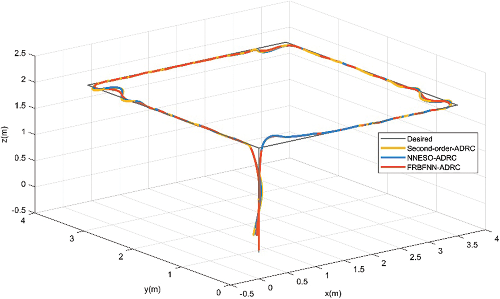
Figure 10: Position tracking of the UAV with a load of 8 kg and no faults
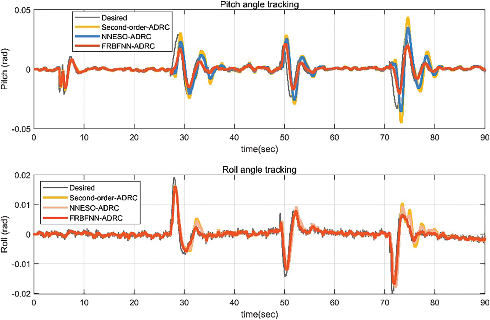
Figure 11: Pitch and roll angles of the UAV with an 8 kg load and no faults
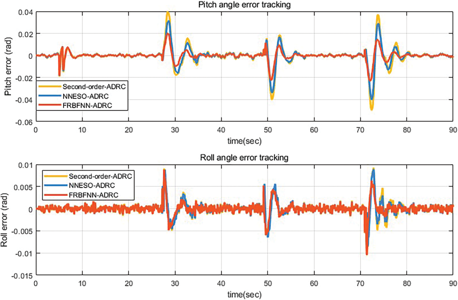
Figure 12: Pitch and roll angle errors of the drone with an 8 kg payload and no faults
In scenario 2, when the UAV unloaded the payload, we injected a 20% gain fault into motors 2 and 3 at the 35th second of flight and injected a 10% bias fault into motors 2 and 3 again at the 60th second. As shown in Fig. 13, both the second-order ADRC controller, NNESO ADRC controller and the proposed fault-tolerant controller still exhibit excellent path-tracking performance during flight. Figs. 14 and 15 reveal that the proposed fault-tolerant controller has smaller errors and better performance during the occurrence of faults.
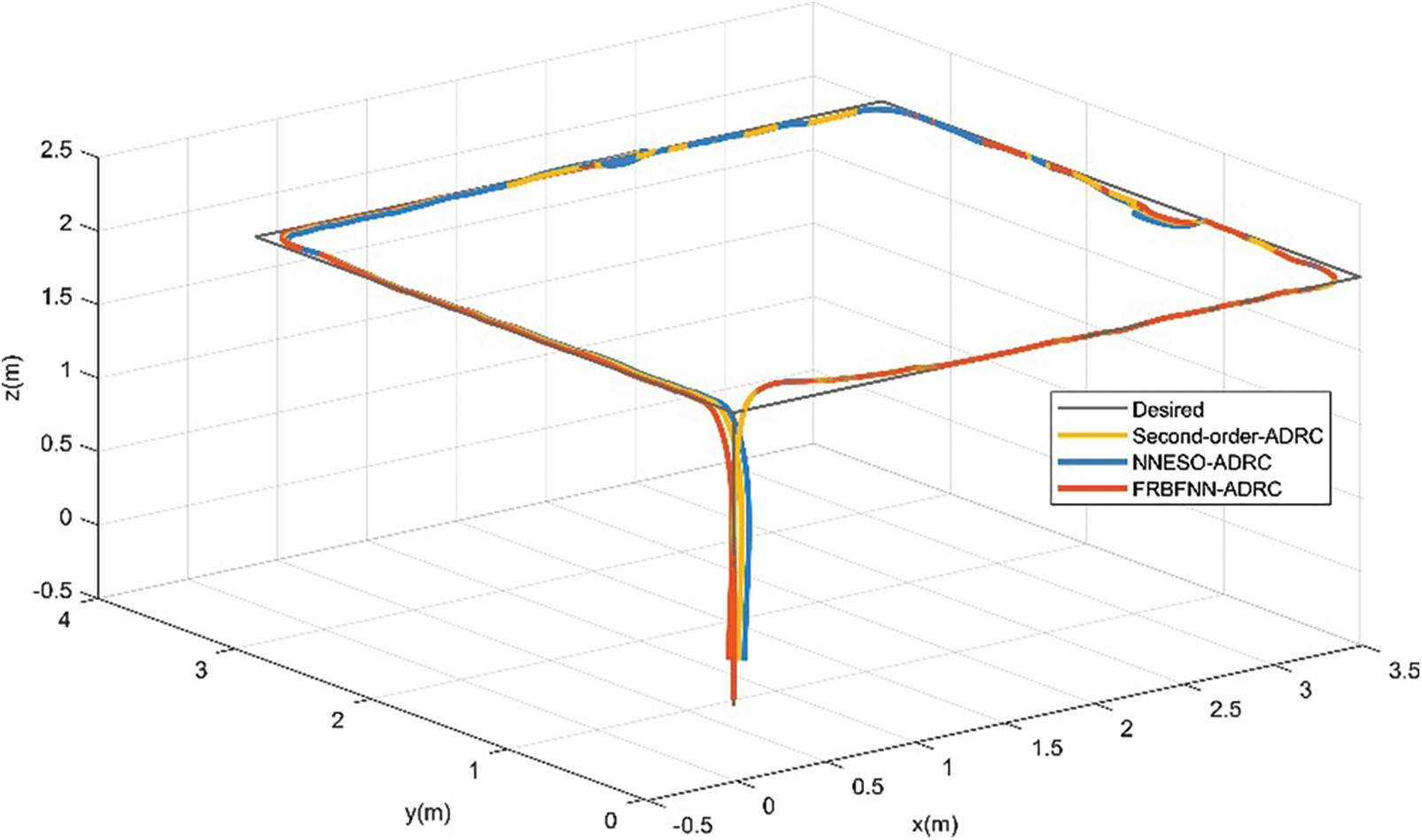
Figure 13: Position tracking of the UAV under actuator faults
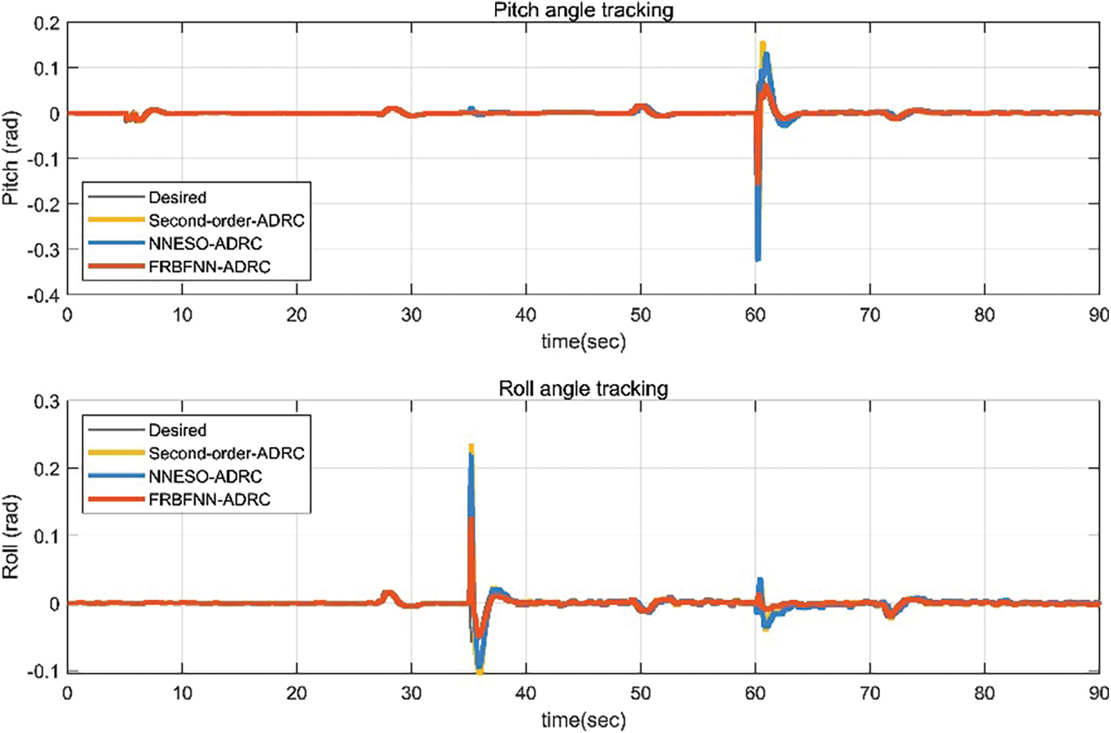
Figure 14: Pitch and roll angles of the UAV with actuator faults
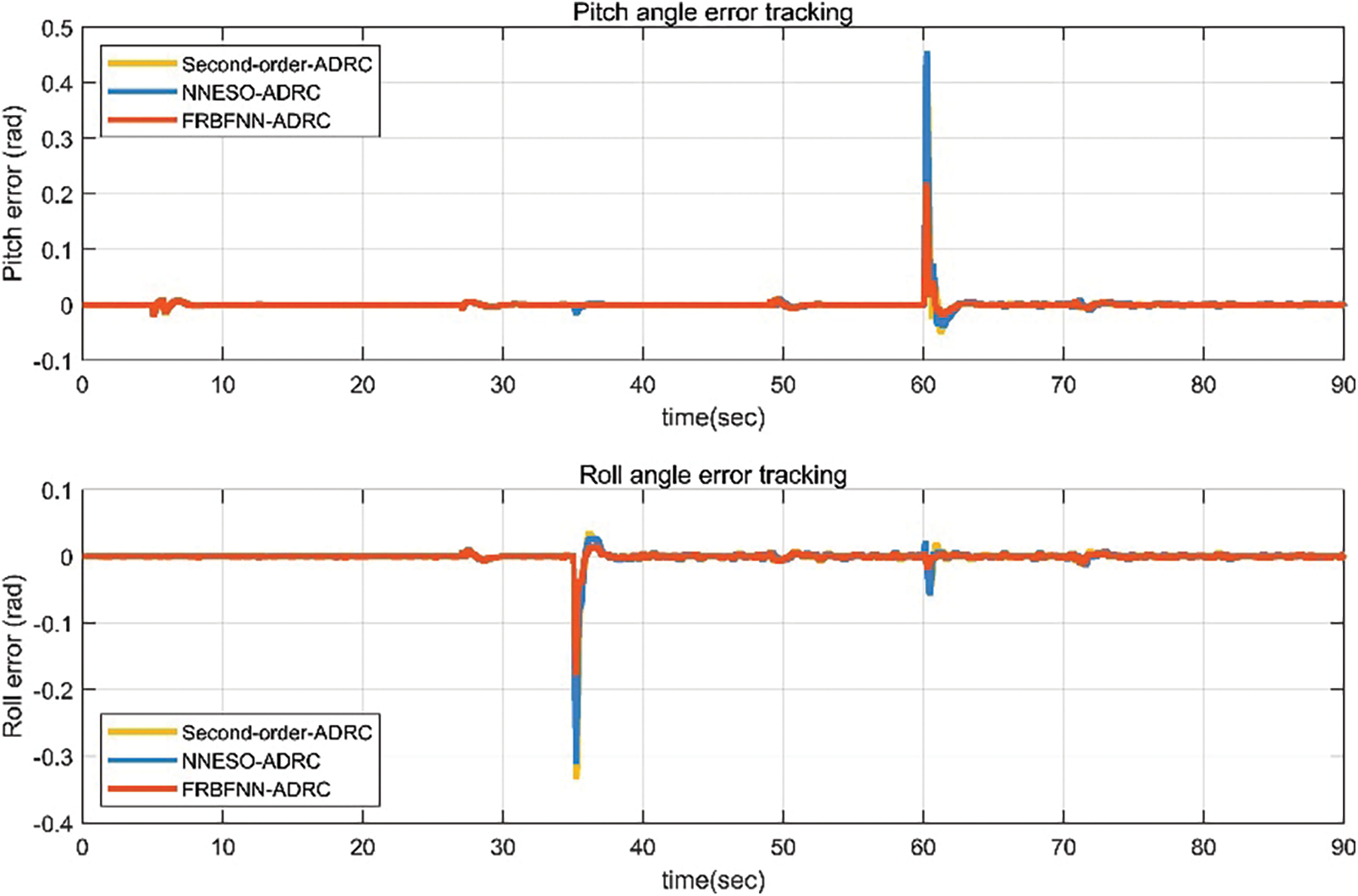
Figure 15: Pitch and roll angle errors of the UAV with actuator faults
In scenario 3, we simulated the situations of load and actuator failures in scenarios 1 and 2, as shown in Fig. 16. At this time, we can compare that the proposed fault-tolerant control algorithm has better path-tracking control and less aircraft oscillation than the second-order ADRC and NNESO ADRC. In Figs. 17 and 18, the attitude and angle tracking errors of the aircraft further demonstrate the more stable attitude control ability of the proposed fault-tolerant control algorithm. It can be seen that NNESO ADRC has a certain degree of fault tolerance. Surprisingly, due to the dual effects of payload disturbance and actuator failure, the controller attitude collapsed when the NNESO ADRC controller injected a bias fault.
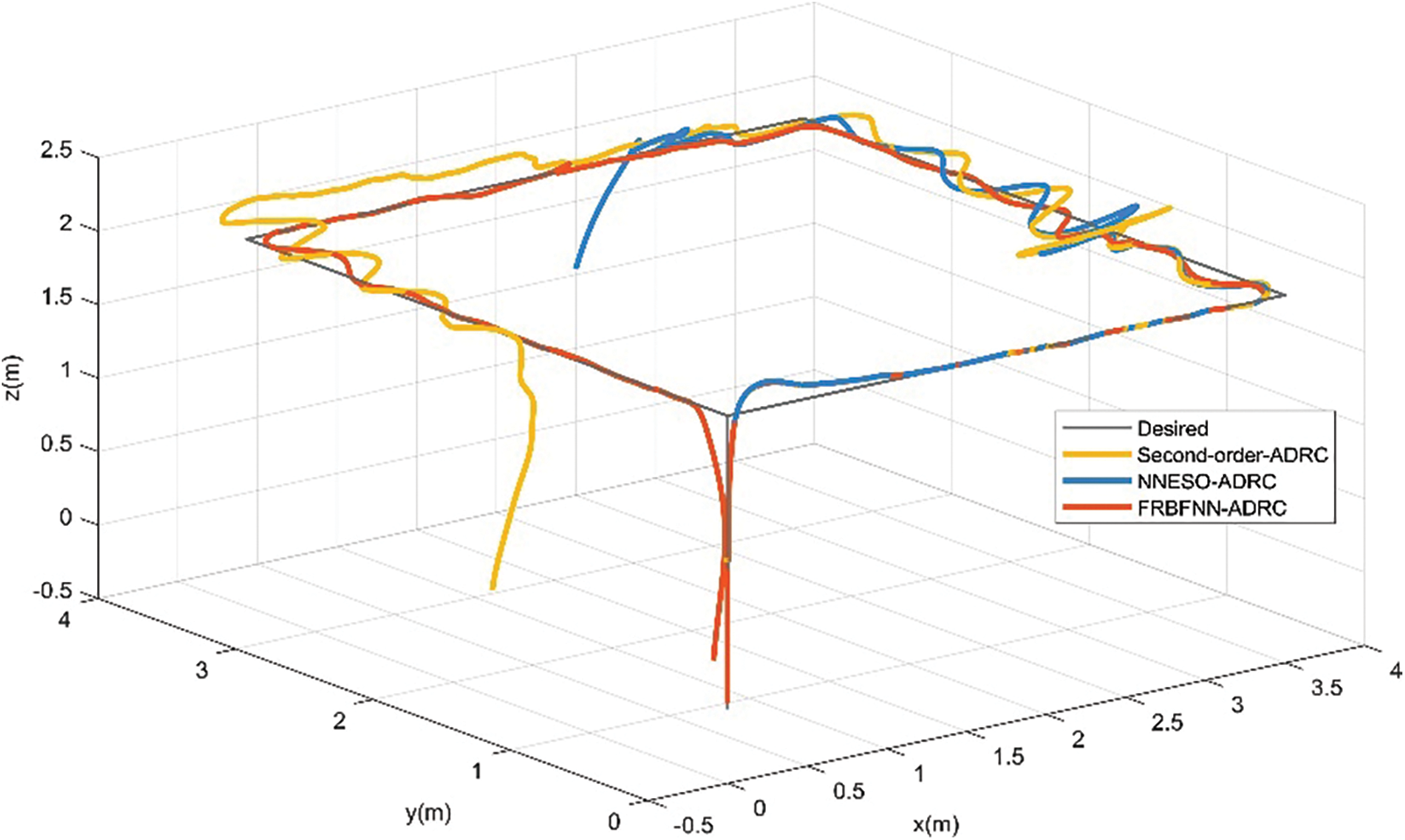
Figure 16: Position tracking of UAV with actuator faults and payload
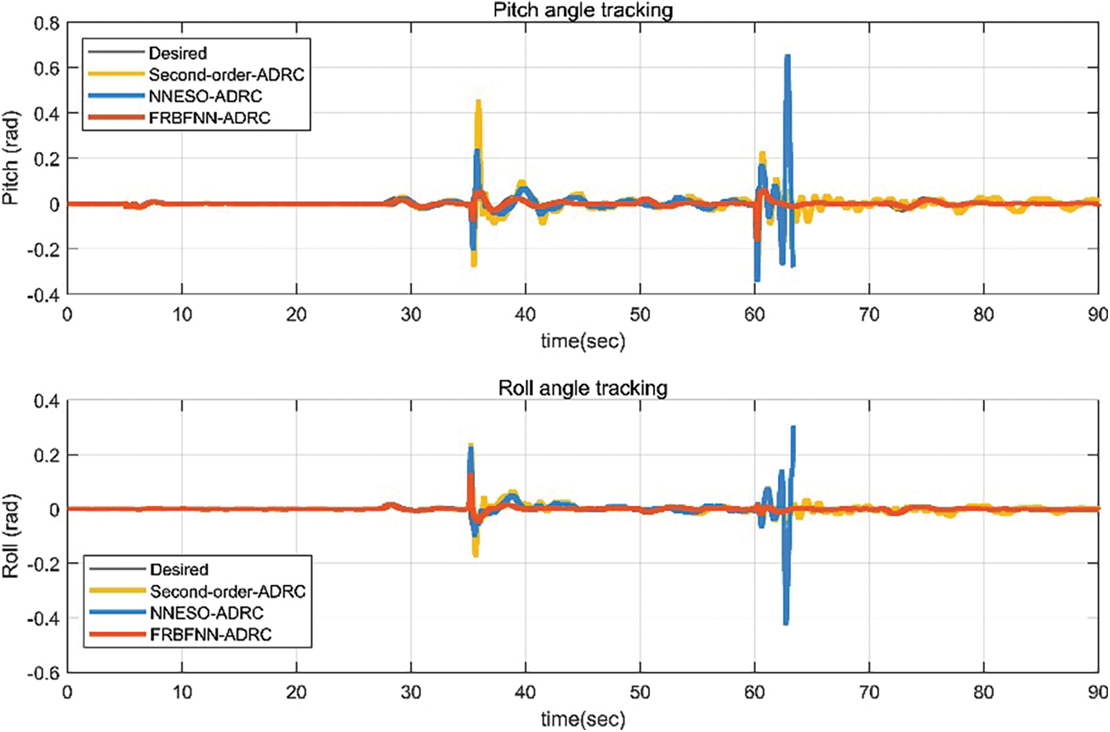
Figure 17: Pitch and roll angles of UAV with actuator faults and payload
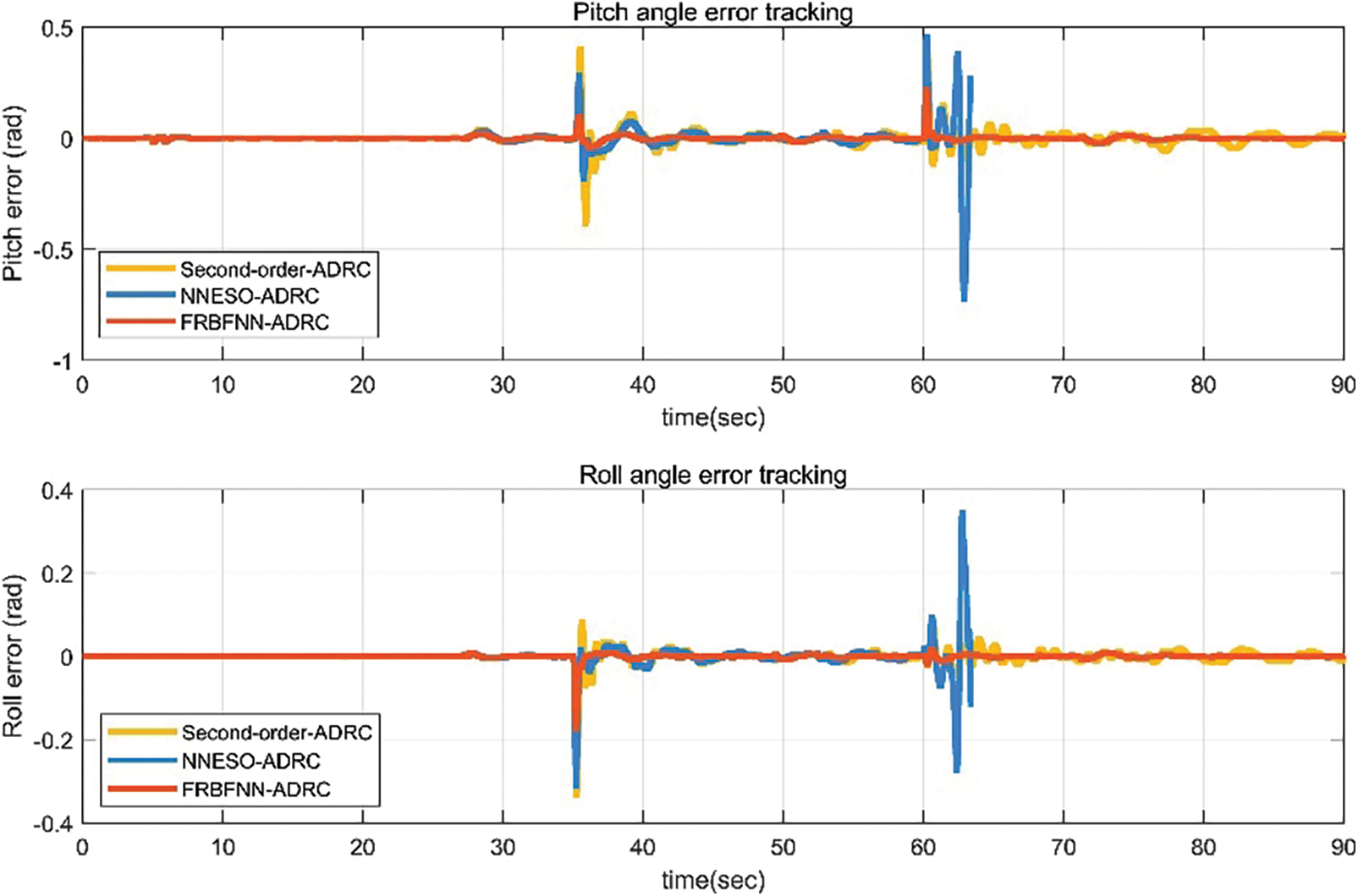
Figure 18: Pitch and roll angle errors of UAV with actuator faults and payload
The observer estimation curves of the pitch and roll subsystems shown in Figs. 19 and 20 are compared with the estimated value

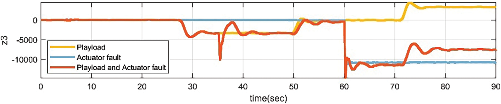
Figure 19: Estimated values of the pitch axis observer in three scenarios for the UAV
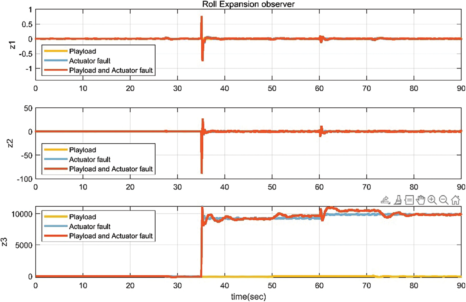
Figure 20: Estimated values of roll axis observer in three scenarios for the UAV

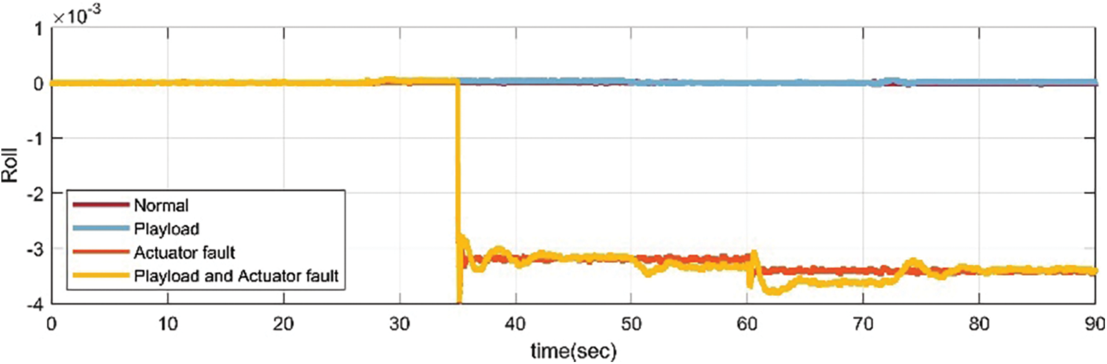
Figure 21: Comparison of pitch and roll control laws for the UAV
Finally, comprehensively analyze the above three scenarios. Comparing the second-order ADRC controller based on traditional RBFNN with the NNESO ADRC controller, it is not difficult to find that both have excellent performance in anti-interference ability. Moreover, in the event of a malfunction, the response speed of each controller is equivalent. However, in terms of accuracy comparison of errors, the FRBFNN ADRC proposed in this paper has smaller errors.
This article presents a novel active fault-tolerant control method based on FRBFNN and a second-order ADRC observer to address actuator bias faults, gain faults, and load disturbance issues in UAVs. The simulation results demonstrate that the designed ADRC controller with playload disturbance suppression capability is a powerful control tool, outperforming other controllers and integrating the uncertain parameters of the actuator model and load disturbance parameters. Furthermore, a new design framework of a self-disturbance fault-tolerant control method with FRBFNN is proposed by combining the traditional and fractional gradient descent methods, taking advantage of the complementary properties of the two. The algorithm’s validity is verified on a multirotor fault-tolerant experimental platform and shows high convergence performance. Comparing the experimental results, it can be found that the proposed fault-tolerant control method has a response speed that is not weaker than other controllers, and has more accurate control tracking ability.
However, the proposed method has certain limitations. Its ability to fully exploit its potential in specific applications depends on the relationship between process dynamics, observer dynamics, sampling time, and measurement noise. On the one hand, the observer must be sufficiently fast compared to the process and closed-loop dynamics to provide more accurate observation values. For example, using an onboard computer for calculating the output of the FRBFNN in this article reduces the impact of the insufficient computing capacity of PIXHAWK4 and greatly improves the accuracy and speed of observer output data. On the other hand, the value of expanding observer poles will be limited by the effect of system sampling frequency and noise on control, which requires a good compromise. In addition, the controller proposed in this article has varying degrees of fault tolerance when actuator failures occur in aircraft with different physical parameter models. Therefore, the follow-up study will seek alternative optimized replacement methods.
Acknowledgement: None.
Funding Statement: This research was funded by the 2021 Key Project of Natural Science and Technology of Yangzhou Polytechnic Institute, Active Disturbance Rejection and Fault-Tolerant Control of Multi-Rotor Plant Protection UAV Based on QBall-X4 (Grant Number 2021xjzk002). 2023 Jiangsu Association for Science and Technology Youth Science and Technology Talent Promotion Project Funded Training Project. Yangzhou City School Cooperation Project “Research on Fault Tolerant Control of Multi Rotor Plant Protection UAV Based on Active disturbance Rejection Technology”.
Author Contributions: The authors confirm contributions to the paper as follows: study conception and design: Lianghao Hua. Jianfeng Zhang; data collection: Dejie Li; analysis and interpretation of results: Lianghao Hua, Jianfeng Zhang, Xiaobo Xi; draft manuscript preparation: Jianfeng Zhang, Xiaobo Xi. All authors reviewed the results and approved the final version of the manuscript.
Availability of Data and Materials: Not applicable.
Conflicts of Interest: The authors declare that they have no conflicts of interest to report regarding the present study.
References
1. Hafeez, A., Husain, M. A., Singh, S. P., Chauhan, A., Mohd, T. K. et al. (2022). Implementation of drone technology for farm monitoring & pesticide spraying: A review. Information Processing in Agriculture, 10(2), 192–203. [Google Scholar]
2. Vargas-Ramírez, N., Paneque-Gálvez, J. (2019). The global emergence of community drones (2012–2017). Drones, 3, 1–24. https://doi.org/10.3390/drones3040076 [Google Scholar] [CrossRef]
3. Gayathri Devi, K., Sowmiya, N., Yasoda, K., Muthulakshmi, K., Kishore, B. (2020). Review on application of drones for crop health monitoring and spraying pesticides and fertilizer. Journal of Critical Reviews, 7, 667–672. https://doi.org/10.31838/jcr.07.06.117 [Google Scholar] [CrossRef]
4. Hassler, S. C., Baisal-Gurrel, F. (2019). Unmanned aerial system (UAS) in agriculture. Agronomy, 9(10), 618. https://doi.org/10.3390/agronomy9100618 [Google Scholar] [CrossRef]
5. San Juan, V., Santos, M., Andújar, J. M. (2018). Intelligent UAV map generation and discrete path planning for search and rescue operations. Complexity, 2018, 1–17. https://doi.org/10.1155/2018/6879419 [Google Scholar] [CrossRef]
6. Wang, Z. G., Zhao, H., Duan, D. G., Jiao, Y. Y., Li, J. B. (2020). Application of improved active disturbance rejection control algorithm in tilt quad rotor. Chinese Journal of Aeronautics, 33(6), 1625–1641. https://doi.org/10.1016/j.cja.2020.01.002 [Google Scholar] [CrossRef]
7. Sierra-García, J. E., Santos, M. (2021). Intelligent control of an UAV with a cable-suspended load using a neural network estimator. Expert Systems with Applications, 183, 115380. https://doi.org/10.1016/j.eswa.2021.115380 [Google Scholar] [CrossRef]
8. Ameya, R. G., Kamesh, S. (2019). Nonlinear control of unmanned aerial vehicles with cable suspended payloads. Aerospace Science and Technology, 93, 105299. https://doi.org/10.1016/j.ast.2019.07.032 [Google Scholar] [CrossRef]
9. Jasim, O. A., Veres, S. M. (2020). A robust controller for multi rotor UAVs. Aerospace Science and Technology, 105, 1270–9638. https://doi.org/10.1016/j.ast.2020.106010 [Google Scholar] [CrossRef]
10. Park, S., Lee, S., Im, B., Lee, D., Shin, S. (2023). Improvement of a multi-rotor UAV flight response simulation influenced by gust. Aerospace Science and Technology, 134, 1270–9638. https://doi.org/10.1016/j.ast.2023.108156 [Google Scholar] [CrossRef]
11. Papachristos, C., Alexis, K., Tzes, A. (2011). Design and experimental attitude control of an unmanned tilt-rotor aerial vehicle. IEEE 15th International Conference on Advanced Robotics: New Boundaries for Robotics, 465–470. https://doi.org/10.1109/icar.2011.6088631 [Google Scholar] [CrossRef]
12. Merheb, A. R., Noura, H., Bateman, F. (2014). Active fault tolerant control of quadrotor UAV using sliding mode control. International Conference on Unmanned Aircraft Systems, 156–166. https://doi.org/10.1109/icuas.2014.6842251 [Google Scholar] [CrossRef]
13. Wen, H., Liang, Z., Zhou, H., Li, X., Yao, B. et al. (2023). Adaptive sliding mode control for unknown uncertain non-linear systems with variable coefficients and disturbances. Communications in Nonlinear Science and Numerical Simulation, 121, 107225. https://doi.org/10.1016/j.cnsns.2023.107225 [Google Scholar] [CrossRef]
14. Xu, W. H., Cao, L. J., Peng, B. Y., Wang, L., Gen, C. et al. (2023). Adaptive nonsingular fast terminal sliding mode control of aerial manipulation based on nonlinear disturbance observer. Drones, 7(2), 88. https://doi.org/10.3390/drones7020088 [Google Scholar] [CrossRef]
15. Zhou, L. S., Ma, L. L., Wang, J. Z. (2017). Fault tolerant control for a class of nonlinear system based on active disturbance rejection control and RBF neural networks. Chinese Control Conference, pp. 7321–7326. Dalian, China. https://doi.org/10.23919/ChiCC.2017.8028513 [Google Scholar] [CrossRef]
16. Zhong, Y. J., Liu, Z. X., Zhang, Y. M., Zhang, W., Zuo, J. Y. (2019). Active fault-tolerant tracking control of a quadrotor with model uncertainties and actuator faults. Frontiers of Information Technology & Electronic Engineering, 20(1), 95–106. https://doi.org/10.1631/FITEE.1800570 [Google Scholar] [CrossRef]
17. Wang, X., Sun, H., Long, Y. W., Zheng, L. H., Liu, H. J. et al. (2018). Development of visualization system for agricultural UAV crop growth information collection. IFAC-PapersOnLine, 51(17), 631–636. https://doi.org/10.1016/j.ifacol.2018.08.126 [Google Scholar] [CrossRef]
18. Antonella, B., Marko, C., Stjepan, B. (2019). Vision-based system for a real-time detection and following of UAV. arXiv:2205.00083. [Google Scholar]
19. Torsten, F., Hans-Jurgen, S., Rudiger, S. (2019). Advances in the development of an industrial UAV for large-scale near-field antenna measurements. 13th European Conference on Antennas and Propagation (EuCAP), pp. 1–3. Krakow, Poland. [Google Scholar]
20. Ding, M. L., Tang, L., Zhou, L. J., Wang, X. M., Weng, Z. L. et al. (2019). W band mini-SAR on multi rotor UAV platform. Proceedings of 2019 IEEE 2nd International Conference on Electronic Information and Communication Technology, pp. 416–418. Harbin, China. https://doi.org/10.1109/iceict.2019.8846356 [Google Scholar] [CrossRef]
21. Lu, H. C., Chang, M. H., Tsai, C. H. (2011). Adaptive self-constructing fuzzy neural network controller for hardware implementation of an inverted pendulum system. Applied Soft Computing, 11(5), 3962–3975. https://doi.org/10.1016/j.asoc.2011.02.025 [Google Scholar] [CrossRef]
22. Liu, L., Liu, Y., Zhou, L., Wang, B., Cheng, Z. et al. (2022). Cascade ADRC with neural network-based ESO for hypersonic vehicle. Journal of the Franklin Institute, 360(12), 9115–9138. https://doi.org/10.1016/j.jfranklin.2022.09.019 [Google Scholar] [CrossRef]
23. Yu, X., Fu, Y., Li, P., Zhang, Y. M. (2018). Fault-tolerant aircraft control based on self-constructing fuzzy neural networks and multivariable SMC under actuator faults. IEEE Transactions on Fuzzy Systems, 26(4), 2324–2335. https://doi.org/10.1109/tfuzz.2017.2773422 [Google Scholar] [CrossRef]
24. Li, T., Zhang, Y. M., Gordon, B. W. (2012). Nonlinear fault-tolerant control of a quadrotor UAV based on sliding mode control technique. IFAC Proceedings Volumes, 8(1), 1317–1322. https://doi.org/10.3182/20120829-3-mx-2028.00056 [Google Scholar] [CrossRef]
25. Wang, J., Zhao, Z. H., Zheng, Y. (2018). NFTSM-based fault tolerant control for quadrotor unmanned aerial vehicle with finite-time convergence. IFAC-PapersOnLine, 51(24), 441–446. https://doi.org/10.1016/j.ifacol.2018.09.614 [Google Scholar] [CrossRef]
26. Amoozgar, M. H., Chamseddine, A., Zhang, Y. M. (2012). Fault-tolerant fuzzy gain-scheduled PID for a quadrotor helicopter testbed in the presence of actuator faults. IFAC Proceedings Volumes, 2(1), 282–2870. https://doi.org/10.3182/20120328-3-it-3014.00048 [Google Scholar] [CrossRef]
27. Boche, A., Farges, J. L., de Plinval, H. (2017). Reconfiguration control method for multiple actuator faults on UAV. IFAC-PapersOnLine, 50(1), 12691–12697. https://doi.org/10.1016/j.ifacol.2017.08.2257 [Google Scholar] [CrossRef]
28. Wen, S. P., Chen, M. Z. Q., Zeng, Z. G., Huang, T. W., Li, C. J. (2017). Adaptive neural-fuzzy sliding-mode fault-tolerant control for uncertain nonlinear systems. IEEE Transactions on Systems Man Cybernetics-Systems, 47(8), 2268–2278. https://doi.org/10.1109/tsmc.2017.2648826 [Google Scholar] [CrossRef]
29. Xiang, Y., Zhang, Y. M. (2015). Design of passive fault-tolerant flight controller against actuator failures. Chinese Journal of Aeronautics, 28(1), 180–190. https://doi.org/10.1016/j.cja.2014.12.006 [Google Scholar] [CrossRef]
30. Ai, S., Song, J., Cai, G., Zhao, K. (2022). Active fault-tolerant control for quadrotor UAV against sensor fault diagnosed by the auto sequential random forest. Aerospace, 9, 518. https://doi.org/10.3390/aerospace9090518 [Google Scholar] [CrossRef]
31. Hua, L. H., Zhang, J. F., Li, D. J., Xi, X. B. (2021). Fault-tolerant active disturbance rejection control of plant protection of unmanned aerial vehicles based on a spatio-temporal RBF neural network. Applied Sciences, 11(9), 4084. https://doi.org/10.3390/app11094084 [Google Scholar] [CrossRef]
32. Wang, S. B., Han, Y., Chen, J., Du, N., Pan, Y. et al. (2018). Flight safety strategy analysis of the plant protection UAV. IFAC-PapersOnLine, 51(17), 262–267. https://doi.org/10.1016/j.ifacol.2018.08.170 [Google Scholar] [CrossRef]
33. Guerrero-Sánchez, M. E., Hernández-González, O., Valencia-Palomo, G., Mercado-Ravell, D. A., López-Estrada, F. R. et al. (2021). Robust IDA-PBC for under-actuated systems with inertia matrix dependent of the unactuated coordinates: Application to a UAV carrying a load. Nonlinear Dynamics, 105, 3225–3238. https://doi.org/10.1007/s11071-021-06776-7 [Google Scholar] [CrossRef]
34. Guerrero-Sanchez, M. E., Lozano, R., Castillo, P., Hernandez-Gonzalez, O., Garcia-Beltran, C. D. et al. (2021). Nonlinear control strategies for a UAV carrying a load with swing attenuation. Applied Mathematical Modelling, 91, 709–722. https://doi.org/10.1016/j.apm.2020.09.027 [Google Scholar] [CrossRef]
35. Herbst, G. (2013). A simulative study on active disturbance rejection control (ADRC) as a control tool for practitioners. Electronics, 2(3), 246–279. https://doi.org/10.3390/electronics2030246 [Google Scholar] [CrossRef]
36. Haykin, S. O. (1994). Neural networks: A comprehensive foundation. Upper Saddle River: Prentice Hall PTR. [Google Scholar]
37. Aftab, W., Moinuddin, M., Shaikh, M. S. (2014). A novel kernel for RBF based neural networks. Abstract and Applied Analysis, 2014, 1–10. https://doi.org/10.1155/2014/176253 [Google Scholar] [CrossRef]
Cite This Article
 Copyright © 2024 The Author(s). Published by Tech Science Press.
This work is licensed under a Creative Commons Attribution 4.0 International License , which permits unrestricted use, distribution, and reproduction in any medium, provided the original work is properly cited.
 Downloads
 Citation Tools