
 Submit a Paper
 Propose a Special lssue
 Open Access
ARTICLE
Euler’s First-Order Explicit Method–Peridynamic Differential Operator for Solving Population Balance Equations of the Crystallization Process
1 Mathematics & Statistics School, Henan University of Science & Technology, Luoyang, 471023, China
2 Longmen Laboratory, Luoyang, 471023, China
3 College of Vehicle and Traffic Engineering, Henan University of Science & Technology, Luoyang, 471023, China
* Corresponding Author: Chunlei Ruan. Email:
(This article belongs to the Special Issue: Peridynamics and its Current Progress)
Computer Modeling in Engineering & Sciences 2024, 138(3), 3033-3049. https://doi.org/10.32604/cmes.2023.030607
Received 14 April 2023; Accepted 18 August 2023; Issue published 15 December 2023
 View Full Text
 Download PDF
Abstract
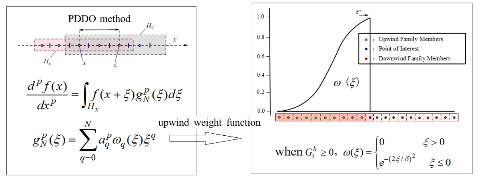
Using Euler’s first-order explicit (EE) method and the peridynamic differential operator (PDDO) to discretize the time and internal crystal-size derivatives, respectively, the Euler’s first-order explicit method–peridynamic differential operator (EE–PDDO) was obtained for solving the one-dimensional population balance equation in crystallization. Four different conditions during crystallization were studied: size-independent growth, size-dependent growth in a batch process, nucleation and size-independent growth, and nucleation and size-dependent growth in a continuous process. The high accuracy of the EE–PDDO method was confirmed by comparing it with the numerical results obtained using the second-order upwind and HR-van methods. The method is characterized by non-oscillation and high accuracy, especially in the discontinuous and sharp crystal size distribution. The stability of the EE–PDDO method, choice of weight function in the PDDO method, and optimal time step are also discussed.Graphic Abstract
Keywords
Crystallization is a low-energy-consumption process that yields products of high purity. This process is employed in various fields, such as chemical industries, medicine, and biotechnology, and involves finer aspects, such as the nucleation and growth of crystals. The population balance equation (PBE) is a mathematical model that describes the crystal size distribution. An accurate solution of the PBE is important to understand and optimize the crystallization process for the improvement of product quality and minimization of production costs.
At present, a large number of numerical results exist in the study of the PBE. They can be roughly divided into three categories based on the numerical method involved: (i) the Monte Carlo method [1,2], (ii) the method of moments [3,4], and (iii) the discrete method [5–7]. The Monte Carlo method uses a large number of random samplings to solve the PBE and can be directly used to analyze multidimensional cases. Thus, the method has several applications in solving the PBE and two-phase flows [8,9]. However, this method is computationally expensive, is prone to generating noise, and hinders coupling with other equations. The method of moments is used to solve the equations for the various moments of the size-distribution function. It has been reviewed by Li et al. [4]. This method is computationally efficient, but reconstructing the size-distribution function from the moments is challenging [10]. Common examples of the method of moments are the quadrature method of moments [11,12] and direct quadrature method of moments [13]. The discrete method directly solves the PBE with the size-distribution function. This method discretizes the internal coordinates and obtains the size-distribution function directly by applying one of the following methods: the finite volume method [14,15], finite element method [16,17], collocation method [18,19], or lattice Boltzmann method [20]. This study focuses on the discrete method for solving the PBE. Since the PBE is a convection-reaction equation in mathematics, its strong hyperbolic property challenges the numerical method. Due to the strong hyperbolic nature of the equation, numerical schemes inevitably cause numerical dissipation and dispersion problems when solving such problems. Traditionally, this problem is solved by using a scheme called the upwind scheme. When calculating derivatives, it only calls more points from the upwind direction of the flow. Besides, the crystallization simulation also contain sharp crystal size distributions and discontinuities. Thus, the high resolution method are required.
The peridynamic differential operator (PDDO) method, a nonlocal differential operator [21–23], has been developed in recent years based on the concept of the peridynamics (PD) theory [24,25]. It connects local partial derivatives and nonlocal integrals through Taylor series expansions and the property of orthogonal functions. The PDDO method can be used to solve differential equations and derive smooth functions or scattered data from discontinuities or singular points. Thus, this method has been successfully applied to the study of stress analysis [26], heat and mass transfer [27], and thermodynamic problems [28]. Recently, Baryt et al. [29] modified the weight function of the PDDO based on the characteristics of hyperbolic equations and obtained a generalized PDDO scheme to accurately solve these equations. Herein, we attempt to apply this method to solve the PBE. The reason we use the PDDO method for dealing with the internal crystal-size derivatives in PBE is that the PDDO method has the ability to deal with the discontinuity in mathematical concepts. Besides, the PDDO can determine any arbitrary order of derivatives regardless of the presence of jump discontinuities or singularities. Also, the PDDO is free of the requirement of symmetric kernels; thus, it eliminates the necessity of ghost particles near the boundary.
In this study, the Euler’s first-order explicit (EE) method and PDDO method are combined (EE–PDDO) to solve the one-dimensional (1D)-PBE, and four cases are presented: (i) size-independent growth, (ii) size-dependent growth in a batch process, (iii) nucleation and size-independent growth, and (iv) nucleation and size-dependent growth in a continuous process. The effectiveness and high accuracy of the EE–PDDO method are verified by comparing it to the analytical solution and other numerical results. The stability of the EE–PDDO method, the weight function in the PDDO scheme, and the optimal time step size are discussed.
2 Population Balance Equation and Numerical Schemes
2.1 Population Balance Equation
The 1D-PBE is expressed as Eq. (1) [14,30].
where
The PD theory is a nonlocal theory proposed by Silling et al. [31]. Point
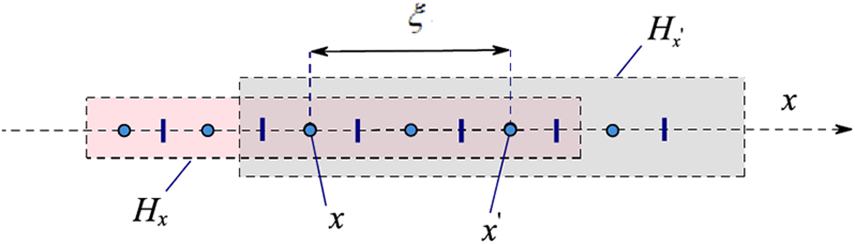
Figure 1: PD interaction domains for the discretized Points x and x′
Madenci et al. [24,25] proposed the PDDO method based on the PD theory. The N-order Taylor series expansions of scalar fields
where
The PD function must be orthogonal to each term in the Taylor series expansions as shown in Eq. (4).
where
where
The unknown coefficient
where
The PDDO method recovers local differentiation as the family size
2.3 EE–PDDO Method for Solving the Population Balance Equation
We initially introduced the internal coordinate grid points for computing the solution and labeled them sequentially as
We evaluated the differential Eq. (1) at the point
The EE method was used for the time derivative to obtain Eq. (9).
where
The PDDO method is used to discretize the internal crystal-size derivative. Taking the polynomial degree N = 1, we have Eq. (10).
where the PD function is constructed using Eq. (5).
The direction of characteristics must be considered when solving hyperbolic equations. Baryt et al. [29] constructed an upwind weight function according to the direction of the incoming flow, when
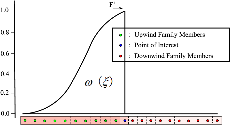
Figure 2: Diagram of the upwind weight function
Again, when
2.4 Stability Analysis of the EE–PDDO Method
The simplest form of the PBE is shown in Eq. (12).
Taking the horizon
We obtain the coefficients for the PD function using Eqs. (6), (7) and (11) as shown in Eq. (15).
The numerical scheme of Eq. (12) is obtained as shown in Eq. (16).
with
We now use the Fourier analysis to show the stability [32]. Let
The stability requirement is
Similarly, when one set of the horizon is
The stability condition is shown in Eq. (20).
Herein we discuss internal crystal-size discretization, for which the treatment of the time derivative is the same as that in the EE method.
2.5.1 Second-Order Upwind Scheme
In the calculation of
In the calculation of
where
We compared the accuracy of each numerical method by defining the following error shown in Eq. (23).
where
3.1 Size-Independent of Growth in a Batch Process
The first example is the crystallization in a batch process where the crystal growth G is independent of crystal size L. We neglected aggregation, nucleation, and breakage, and set
3.1.1 Single-Mode with Non-Smooth Distribution
The initial crystal-size function satisfies the non-smooth distribution shown in Eq. (24) [33].
In the calculation, the domain is set as
Fig. 3 shows the comparison of the exact solution with the results obtained by four numerical schemes at t = 60 s. The time step is chosen as Δt = 0.05 s in the first-order upwind, second-order upwind and HR-van schemes owing to the differences in the stability condition. The time step is chosen as
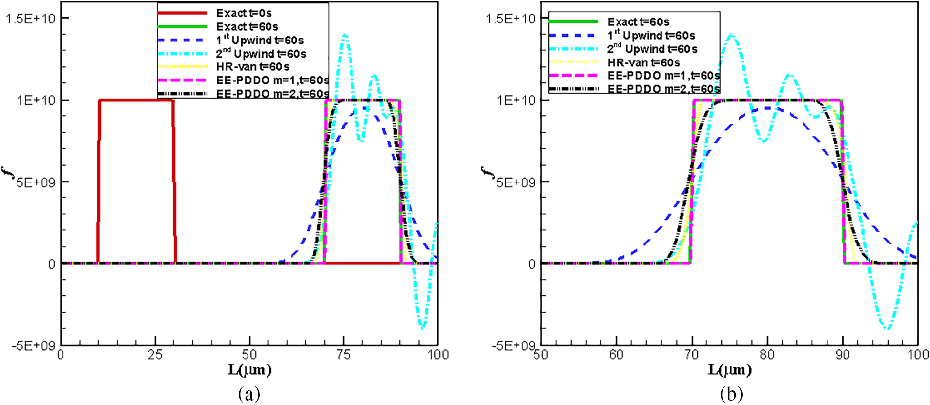
Figure 3: Comparison of analytical and numerical crystal size distribution. (a) In the whole computational zone (b) zoomed figure
Fig. 4 shows the evolution of L2 error of different numerical schemes with the time steps at t = 60 s. The EE–PDDO method with m = 2 has the larger stability region, which means Δt can be the larger. The second-order upwind scheme has the smaller stability region. The EE–PDDO method with m = 1 has the smaller error at
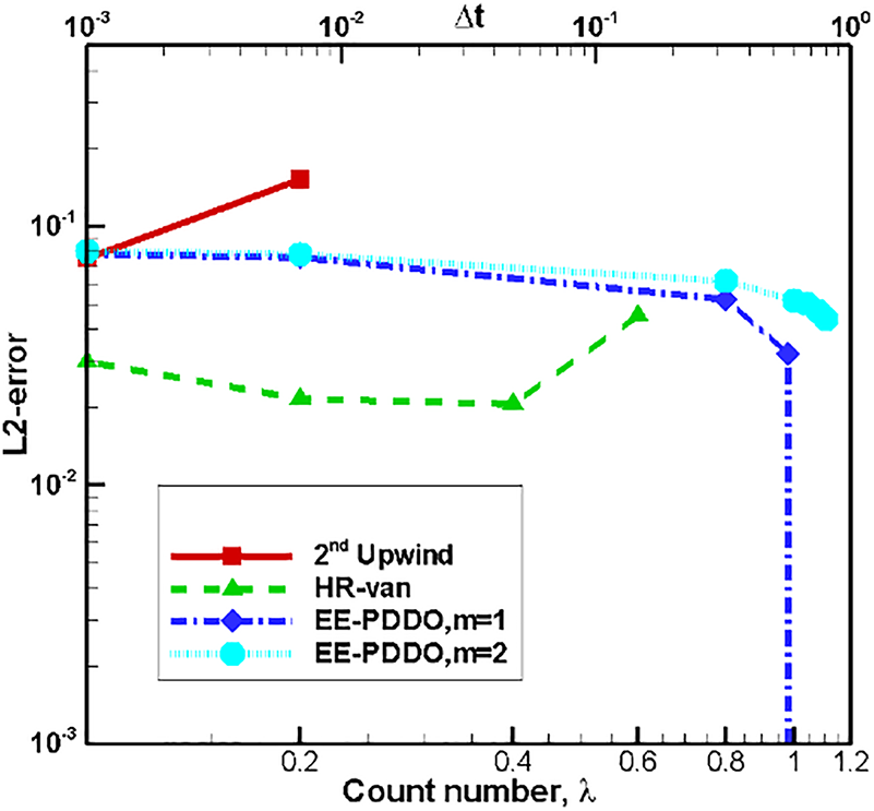
Figure 4: Evolution of the L2 error of different numerical schemes with the time steps
The method of directly solving the crystal size distribution function is often considered to be too expensive to couple with Computational fluid dynamics (CFD) [18,34]. Therefore, we now focus on the CPU time for these methods. Fig. 5 shows the CPU time of three methods with different numbers of internal crystal-size points. Since the stability conditions of these methods are different, the time step is selected as mentioned here: (i)
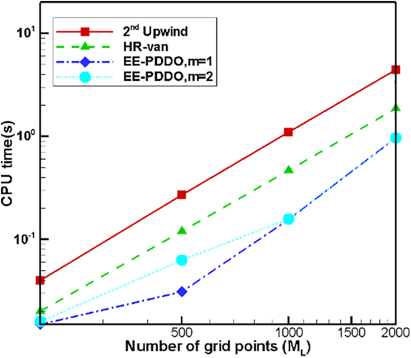
Figure 5: Evolution of the required CPU time with the number of internal crystal-size points for different schemes
Therefore, it is best to select the EE–PDDO method with m = 1 and Δt = ΔL in the case of size-independent growth from the perspective of accuracy and efficiency. When
3.1.2 Multi-Modal with Non-Smooth Distribution
The initial crystal size function of the multi-modal case is assumed as Eq. (25) [33]:
The computational zone is set as
The other parameters are set as shown here:
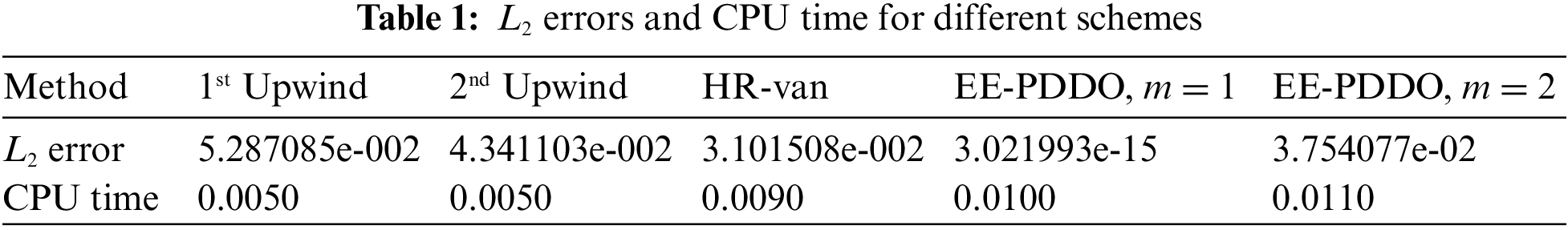
Fig. 6 shows the comparison of the analytical solution with numerical solutions obtained by different schemes at t = 100 s. The result of the EE–PDDO method with m = 1 is also a reproduction of the exact solution, while the result of the EE–PDDO method with m = 2 is similar to that of the HR-van method. Table 1 lists the L2 error and the CPU time for different schemes. From the perspective of accuracy and efficiency, the EE–PDDO method with m = 1 is also the best choice. Also, as shown in Table 1, the accuracy of the second-order upwind is sightly better than that of the first-order upwind. Therefore, we shall not show the performance of the first-order upwind scheme in the following examples.
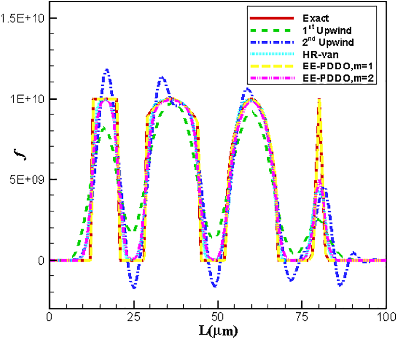
Figure 6: Comparison of analytical and numerical crystal size distribution
3.2 Size-Dependent Growth in a Batch Process
We have considered the example of G dependent on L in a batch process. Aggregation, nucleation, and breakage are not considered. Thus,
The initial size distribution satisfies Eq. (27).
where
We set the parameters as
Fig. 7 shows the comparison of the numerical solutions of different schemes with the analytical solution at t = 4 s. Here, the normal weight in the EE–PDDO method is the weight function considered as
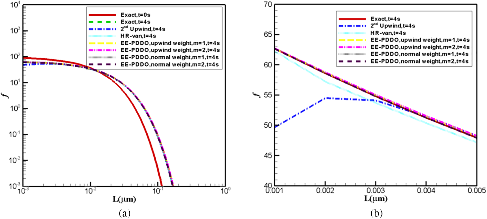
Figure 7: Comparison of analytical and numerical crystal size distribution. (a) In the whole computational zone (b) zoomed figure
Fig. 8 shows the
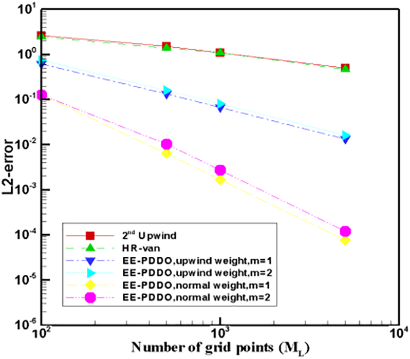
Figure 8: Evolution of the L2 error with the number of spatial points for different schemes
The PBE becomes a convection-reaction equation in the size-dependent growth case due to the dependency of G and L. Thus, its hyperbolic property decreases. The equation can be solved using regular numerical schemes. Therefore, the EE–PDDO method with the normal weight function is the most appropriate choice for the simulation of size-dependent growth cases.
3.3 Nucleation and Size-Independent Growth in a Continuous Process
The PBE is expressed as Eq. (29) considering the nucleation and size-independent growth in a continuous process.
where the source term is
where
The initial distribution is
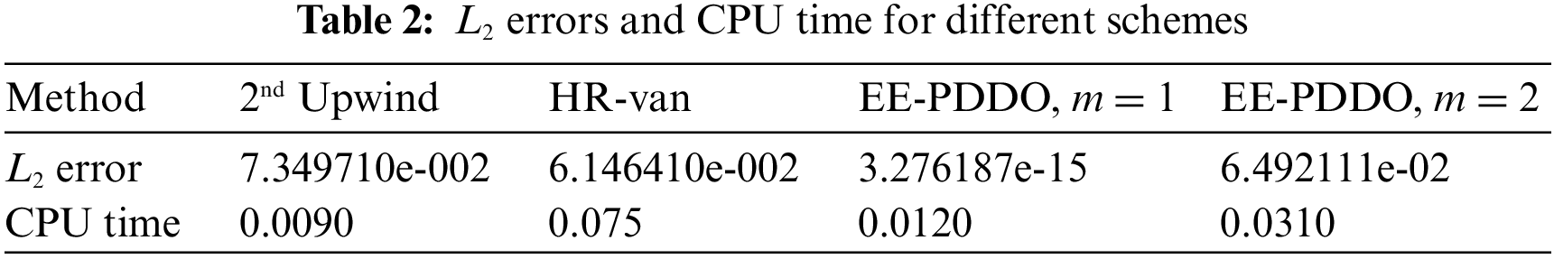
Fig. 9 shows the comparison of analytical and numerical crystal-size distributions. The EE–PDDO method with m = 1 has a strong ability to accurately capture the discontinuous states. Although for m = 2 in EE–PDDO method, the solution is poorer than that of the HR-van method, the solution is non-oscillating. Table 2 lists the L2 errors and CPU time for different schemes. The advantages of the EE–PDDO method are high accuracy and efficiency.
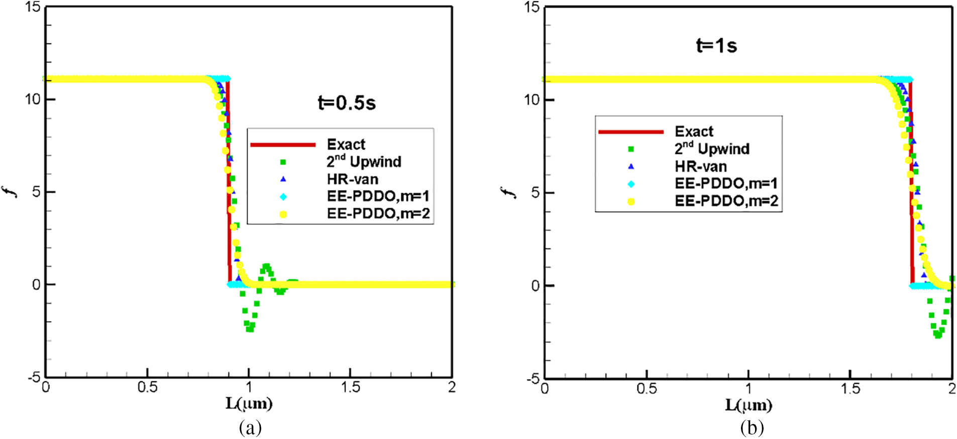
Figure 9: Comparison of analytical and numerical crystal size distribution: (a) t = 0.5 s and (b) t = 1 s
3.4 Nucleation and Size-Dependent Growth in a Continuous Process
The corresponding PBE for the nucleation and size-dependent growth in a continuous process is given by Eq. (31).
The source term is assumed as
The initial distribution was assumed to be given by Eq. (32) and the simulation ended at t = 10000 s. The computational domain is set as [0, 4 μm]. The other parameters are set as shown here:
Fig. 10 shows the comparison between the analytical and numerical solutions obtained by the three schemes. Fig. 10a indicates that all the numerical results are in good agreement with the exact solutions except for the second-order upwind scheme. This deviation is clear in Fig. 10b.
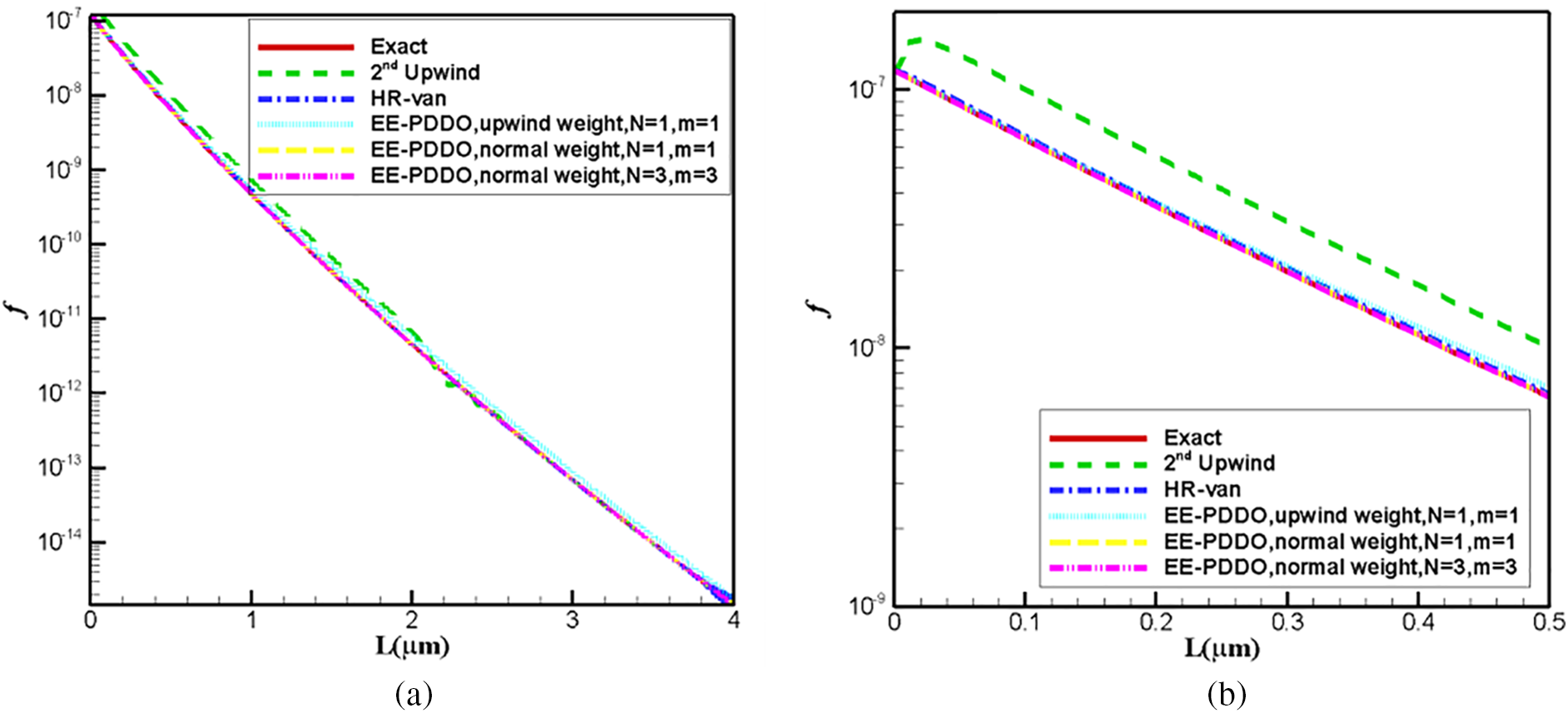
Figure 10: Comparison of analytical and numerical crystal size distribution. (a) In the whole computational zone (b) zoomed figure
Table 3 listed the L2 errors and CPU time for different schemes. The errors of the HR-van scheme and EE–PDDO method with the upwind weight function of m = 1 are close. The corresponding results are poorer than those obtained by the EE–PDDO method with the normal weight function of m = 1. In the EE–PDDO method, the accuracy can be improved by increasing the order of polynomials. When the polynomial order is increased (N = 3), highly accurate numerical results are obtained. The accuracy of EE–PDDO method is determined by parameters. In general, increasing the value of
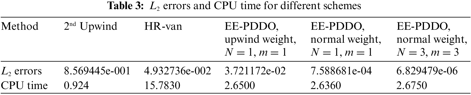
In this size-dependent growth case, the EE–PDDO method with the normal weight function is recommended.
In this paper, the EE–PDDO method for solving 1D-PBE is presented. We studied four different cases: size-independent growth, size-dependent growth in a batch process, nucleation and size-independent growth, and nucleation and size-dependent growth in a continuous process. These cases were solved by the EE–PDDO, second-order upwind, and HR-van methods. The stability of the EE–PDDO method, choice of the weight function in the PDDO method, and optimal time step were discussed. The conclusions are as follows:
(1) The EE–PDDO method has high accuracy and efficiency in solving the 1D-PBE. This method is characterized by non-oscillation and high accuracy, especially in the discontinuous and sharp crystal size distribution.
(2) The stability condition of the EE–PDDO method of the simplest PBE with the size-independent growth case is
(3) The upwind weight function should be used in the PDDO method to reach stability in the size-independent growth case. The time step size is recommended as
We present the EE–PDDO method for solving 1D PBE. The detailed implementation and the corresponding techniques were discussed here. This method is also expected to be used for solving more complex crystallization processes.
Acknowledgement: The authors acknowledge the School of Mathematics and Statistics, Henan University of Science and Technology, for allowing the use of their high-performance computing resources.
Funding Statement: The authors received no specific funding for this study.
Author Contributions: The authors confirm contribution to the paper as follows: study conception and design: Chunlei Ruan, Cengceng Dong; data collection: Kunfeng Liang, Zhijun Liu, Xinru Bao; analysis and interpretation of results: Chunlei Ruan, Cengceng Dong; draft manuscript preparation: Chunlei Ruan, Cengceng Dong. All authors reviewed the results and approved the final version of the manuscript.
Availability of Data and Materials: The data that support the findings of this study are available on request from the corresponding author upon reasonable request.
Conflicts of Interest: The authors declare that they have no conflicts of interest to report regarding the present study.
References
1. Tandon, P., Rosner, D. E. (1999). Monte Carlo simulation of particle aggregation and simultaneous restructuring. Journal of Colloid & Interface Science, 213(2), 273–286. [Google Scholar]
2. Meimaroglou, D., Kiparissides, C. (2007). Monte carlo simulation for the solution of the bi-variate dynamic population balance equation in batch particulate systems. Chemical Engineering Science, 62(18–20), 5295–5299. [Google Scholar]
3. Caliane, B., Maria, R., Rubens, M. (2007). Considerations on the crystallization modeling: Population balance solution. Computers & Chemical Engineering, 31(3), 206–218. [Google Scholar]
4. Li, D. Y., Li, Z. P., Gao, Z. M. (2019). Quadrature-based moment methods for the population balance equation: An algorithm review. Chinese Journal of Chemical Engineering, 27(3), 483–500. [Google Scholar]
5. Kumar, S., Ramkrishna, D. (1997). On the solution of population balance equations by discretization—I. A fixed pivot technique. Chemical Engineering Science, 52, 1311–1332. [Google Scholar]
6. Li, S., Liu, W. K. (1999). Reproducing kernel hierarchical partition of unity, part I—Formulation and theory. International Journal for Numerical Methods in Engineering, 45(3), 251–288. [Google Scholar]
7. Li, S., Liu, W. K. (1999). Reproducing kernel hierarchical partition of unity, part II—Applications. International Journal for Numerical Methods in Engineering, 45(3), 289–317. [Google Scholar]
8. Xu, Z., Zhao, H., Zheng, C. (2014). Fast Monte Carlo simulation for partice coagulation in population balance. Journal of Aerosol Science, 74(4), 11–25. [Google Scholar]
9. Xu, Z., Zhao, H., Zheng, C. (2015). Accelerating population balance-Monte Carlo simulation for coagulation dynamics from the markov jump model, stochastic algorithm and GPU parallel computing. Journal of Computational Physics, 281, 844–863. [Google Scholar]
10. John, V., Angelov, I., Oncul, A., Thevenin, D. (2007). Techniques for the reconstrucion of a distribution from a finite number of its moments. Chemical Engineering Science, 62(11), 2890–2904. [Google Scholar]
11. Lage, P. L. C. (2011). On the representation of QMOM as a weighted residual method—The dual quadrature method of generalized moments. Computers & Chemical Engineering, 35(11), 2186–2203. [Google Scholar]
12. Grosch, R., Briesen, H., Marquardt, M., Wulkow, M. (2007). Generalization and numerical investigation of QMOM. AICHE Journal, 53(1), 207–227. [Google Scholar]
13. Marchisio, D. L., Fox, R. O. (2005). Solution of population balance equations using the direct quadrature method of moments. Journal of Aerosol Science, 36(1), 43–73. [Google Scholar]
14. Gunawan, R., Fusman, I., Braatz, R. D. (2004). High resolution algorithms for multidimensional population balance equations. AICHE Journal, 50(11), 2738–2749. [Google Scholar]
15. Noor, S., Qamar, S. (2015). The space time CE/SE method for solving one-dimensional batch crystallization model with fines dissolution. Chinese Journal of Chemical Engineering, 23(2), 337–341. [Google Scholar]
16. Nicmanis, M., Hounslow, M. J. (1998). Finite-element methods for steady-state population balance equations. AICHE Journal, 44(10), 2258–2272. [Google Scholar]
17. Sandu, A. (2006). Piecewise polynomial solutions of aerosol dynamic equation. Aerosol Science and Technology, 40(4), 261–273. [Google Scholar]
18. Alzyod, S., Charton, S. (2020). A meshless radial basis method (RBM) for solving the detailed population balance equation. Chemical Engineering Science, 228(31), 1–32. [Google Scholar]
19. Ruan, C. (2019). Chebyshev spectral collocation method for population balance equation in crystallization. Mathematics, 7(317), 1–12. [Google Scholar]
20. Majumder, A., Kariwala, V., Ansumali, S., Rajendran, A. (2012). Lattice Boltzmann method for multi-dimensional population balance models in crystallization. Chemical Engineering Science, 70(18), 121–134. [Google Scholar]
21. Gunzburger, M., Lehoucq, R. B. (2010). A nonlocal vector calculus with application to nonlocal boundary value problems. Multiscale Modeling & Simulation, 8(5), 1581–1598. [Google Scholar]
22. Yan, J., Li, S., Kan, X., Zhang, A. M., Lai, X. (2020). Higher-order nonlocal theory of updated lagrangian particle hydrodynamics (ULPH) and simulations of multiphase flows. Computer Methods in Applied Mechanics and Engineering, 368(2), 113176. [Google Scholar]
23. Yu, H., Li, S. (2021). On approximation theory of nonlocal differential operators. International Journal for Numerical Methods in Engineering, 122(23), 6984–7012. [Google Scholar]
24. Madenci, E., Baryt, A., Dorduncu, M. (2019). Peridynamic differential operator for numerical analysis. Switzerland: Springer Nature Switzerland. [Google Scholar]
25. Madenci, E., Baryt, A., Futch, M. (2016). Peridynamic differential operator and its applications. Computer Methods in Applied Mechanics and Engineering, 304, 408–451. [Google Scholar]
26. Dorduncu, M. (2019). Stress analysis of sandwich plates with functionally graded cores using peridynamic differential operator and refined zigzag theory. Thin-Walled Structures, 146, 106468. [Google Scholar]
27. Gao, Y., Oterkus, S. (2019). Nonlocal modeling for fluid flow coupled with heat transfer by using peridynamic differential operator. Engineering Analysis with Boundary Elements, 105(2), 104–121. [Google Scholar]
28. Li, Z. Y., Huang, D., Xu, Y. P. (2021). Nonlocal steady-state thermoelastic analysis of functionally graded materials by using peridynamic differential operator. Applied Mathematical Modelling, 93, 294–313. [Google Scholar]
29. Baryt, A., Madenci, E., Haghighat, E. (2022). On the solution of hyperbolic equations using the peridynamic differential operator. Computer Methods in Applied Mechanics and Engineering, 391, 114574. [Google Scholar]
30. Ma, D. L., Tafti, D. K., Braatz, R. D. (2002). High-resolution simulation of multidimensional crystal growth. Industrial & Engineering Chemistry Research, 41(25), 6217–6223. [Google Scholar]
31. Silling, S. A., Epton, M., Weckner, O. (2007). Peridynamic states and constitutive modeling. Journal of Elasticity, 88(2), 151–184. [Google Scholar]
32. Mark, H. (2011). Introduction to numerical methods in differential equaitons. Berlin: Springer. [Google Scholar]
33. Qamar, S., Elsner, M. P., Angelov, I. A., Warnecke, G., Seidel-Morgenstern, A. (2006). A comparative study of high resolution schemes for solving population balances in crystallization. Computers & Chemical Engineering, 30(6–7), 1119–1131. [Google Scholar]
34. Cheng, J. C., Li, Q., Yang, C., Zhang, Y. Q., Mao, Z. S. (2018). CFD-PBE simulation of a bubble column in OpenFOAM. Chinese Journal of Chemical Engineering, 26(9), 1773–1784. [Google Scholar]
35. Hounslow, M. J. (1988). A discretized population balance for nucleation growth, and aggregation. AIChE Journal, 34, 1576–1589. [Google Scholar]
Cite This Article
 Copyright © 2024 The Author(s). Published by Tech Science Press.
This work is licensed under a Creative Commons Attribution 4.0 International License , which permits unrestricted use, distribution, and reproduction in any medium, provided the original work is properly cited.
 Downloads
 Citation Tools