An Effective Meshless Approach for Inverse Cauchy Problems in 2D and 3D Electroelastic Piezoelectric Structures

1  Introduction

In modern engineering applications, advanced structures incorporating piezoelectric materials have gained widespread utilization and design. The interaction between electrical effects and mechanical deformation is one of the most appealing characteristics of piezoelectric materials. However, traditional mathematical analysis using various analytical and semi-analytical methodologies falls in addressing practical piezoelectric problems [1,2], particularly those involving complex geometry and loading conditions. Hence, the demand for accurate and efficient numerical models becomes imperative [3–7].

In the field of computational mechanics, numerical tools such as the finite difference (FDM) and finite element (FEM) methods have been widely used as the primary techniques for solving various PDEs. However, the traditional FEM and FDM models possess inherent limitations, particularly when it comes to re-meshing processes or dealing with highly distorted elements [8–12]. In the past two decades, substantial efforts have been made to develop innovative computational techniques that overcome or significantly mitigate these issues associated with the classical FEM and FDM. As a result, a multitude of meshless methods have been developed in response to this need [13–17].

During the past few years, the GFDM has emerged as an efficient meshless collocation technique for solving diverse boundary value problems. Its high accuracy and excellent computational efficiency have garnered significant attention from researchers in engineering and mathematical communities. The method’s core idea was initially proposed by Liszka et al. in the early 1980s [18] and has since been extended and refined by numerous others [19–23]. The GFDM involves dividing the entire domain into multiple sub-domains. Within each sub-domain, explicit formulas for the necessary partial derivatives of the PDEs can be obtained through the application of Taylor series expansion and moving-least square approximation methods. The concept of “local star” or “local subdomain” employed in GFDM results in a sparse coefficient matrix, making the method particularly suitable for large-scale computations.

This study represents the pioneering effort to apply GFDM to address the numerical solution of inverse electroelastic analysis concerning both 2D and 3D piezoelectric structures. Solving such problems poses a formidable challenge within the computational mechanics community. The research obstacles stem from the intricate interplay of electroelastic behaviors in piezoelectric materials, as well as the ill-conditioning problem inherent in inverse problems [24–26]. This study will present the numerical procedures of the GFDM, focusing on its application for inverse Cauchy piezoelectric problems. It will demonstrate that the proposed GFDM can achieve accurate and stable solutions for such problems.

2  Inverse Cauchy Problems in 2D and 3D Electroelastic Piezoelectric Structures

2.1 Two-Dimensional (2D) Piezoelectric Problems

Consider a 2D domain bounded by a given boundary Γ=∂Ω. The equilibrium equations for piezoelectric structures can be formulated as follows [27,28]:

σij,j+fi=0,Di,i−q=0,(1)

where σij, fi, Di and q represent the stress tensor, the body force vector per unit volume, the electric displacement vector and the electric charge per unit volume, respectively. The constitutive equation for 2D piezoelectric problems (under the plane strain assumption) can be expressed as follows [28]:

[σ11σ33σ13]=[c11c130c13c33000c44][ε11ε332ε13]−[0e310e33e150][E1E3],(2)

[D1D3]=[00e15e31e330][ε11ε332ε13]+[κ1100κ33][E1E3],(3)

where eij, κij and cij represent the piezoelectric constants, the dielectric tensor and the elastic modulus tensor, respectively, εij and Ei denote the elastic strain tensor and the electric field component which can be obtained by:

εij=12(ui,j+uj,i),Ei=−ϕ,i,(4)

with ϕ and ui represent the electric scalar potential and the displacement component, respectively. Without considering the body force and electric charge, Eq. (1) can be rephrased in terms of ϕ and ui as follows [28]:

[c11∂2∂x2+c44∂2∂z2(c13+c44)∂2∂x∂z(e15+e31)∂2∂x∂z(c13+c44)∂2∂x∂zc44∂2∂x2+c33∂2∂z2e15∂2∂x2+e33∂2∂z2−(e15+e31)∂2∂x∂z−e15∂2∂x2−e33∂2∂z2κ11∂2∂x2+κ33∂2∂z2][u1u3ϕ]=[000],(5)

with the corresponding boundary conditions:

{ui=u¯ionΓuσijnj=t¯ionΓt,and{ϕ=ϕ¯ onΓϕDini=−ω¯ onΓω,(6)

where ω and ti represent surface charge and traction component, respectively, Γ=Γu+Γt=Γϕ+Γω represents the whole surfaces of the domain.

2.2 Three-Dimensional (3D) Piezoelectric Problems

Similarly, for 3D problems, the constitutive equations are as follows [29]:

[σ11σ22σ33σ23σ13σ12]=[c11c12c13000c12c11c13000c13c13c33000000c44000000c44000000c66][ε11ε22ε332ε232ε132ε12]−[00e3100e3100e330e150e1500000][E1E2E3],(7)

[D1D2D3]=[0000e150000e1500e31e31e33000][ε11ε22ε332ε232ε132ε12]+[κ11000κ11000κ33][E1E2E3],(8)

where the relation c11=c12+2c66 should be satisfied. Similarly, the equilibrium equations for 3D piezoelectric problems can be restated in the following manner [29]:

[c11∂2∂x12+c66∂2∂x22+c44∂2∂x32(c12+c66)∂2∂x1∂x2(c13+c44)∂2∂x1∂x3(e31+e15)∂2∂x1∂x3(c12+c66)∂2∂x1∂x2c66∂2∂x12+c11∂2∂x22+c44∂2∂x32(c13+c44)∂2∂x2∂x3(e31+e15)∂2∂x2∂x3(c13+c44)∂2∂x1∂x3(c13+c44)∂2∂x2∂x3c44∂2∂x12+c44∂2∂x22+c33∂2∂x32e15∂2∂x12+e15∂2∂x22+e33∂2∂x32(e31+e15)∂2∂x1∂x3(e31+e15)∂2∂x2∂x3e15∂2∂x12+e15∂2∂x22+e33∂2∂x32−κ11∂2∂x12−κ11∂2∂x22−κ33∂2∂x32][u1u2u3ϕ]=[0000].(9)

In inverse Cauchy problems, only a specific portion of the boundary, referred to as Γ1, is accessible for assessments. Conversely, no information is available for the remaining border Γ2 (under-specified surface). The description of the present GFDM for addressing this type of problem will be introduced in the subsequent section.

3  The Methodology of GFDM

Without loss of generality, we focus on describing the numerical implementation of the GFDM for general 3D problems in this context. However, for 2D problems, the numerical procedures can be found in [28,30]. In the GFDM approach, the first step involves scattering a cloud of points throughout the entire computational domain. Subsequently, the method establishes a series of sub-domains and applies the following procedure to match the solution within each sub-domain.

Let Ω∈R3 represent the computational domain, while M={x1,…,xN}∈Ω denotes a discretization of Ω comprising N nodes in total. In this context, we designate each point in M as a node, specifically named as x0=(x0,y0,z0). For each x0, the m nearest points {xi=(xi,yi,zi)}i=1m around x0 should be determined. The local domain Em then denotes the area that contains points {xi}i=0m. Let’s suppose {Ui=U(xi)}i=0m are unknown functions (displacements or electric scalar potential) defined at points {xi}i=0m, then the values of Ui can be calculated by using the Taylor series expansion:

Ui=U0+hi∂U0∂x+ki∂U0∂y+li∂U0∂z+12(hi2∂2U0∂x2+ki2∂2U0∂y2+li2∂2U0∂z2)+ hiki∂2U0∂x∂y+hili∂2U0∂x∂z+kili∂2U0∂y∂z+…,i=1,…,m(10)

where hi=xi−x0,ki=yi−y0,li=zi−z0. According to Eq. (10), an error function can be defined as:

B(U)=∑i=1m[(U0−Ui+hi∂U0∂x+ki∂U0∂y+li∂U0∂z+…+kili∂2U0∂y∂z)ω(hi,ki,li)]2,(11)

where ω represents weighting functions that diminish in magnitude as the distance from x0 increases [21,22,31]. In our computations, the following weighting functions are chosen [32]:

ω(hi,ki,li)=1−6(didm)2+8(didm)3−3(didm)4,  di≤dm(12)

where di=|x0−xi| and dm=max|x0−xi|. Let us define

DU={∂U0∂x,∂U0∂y,∂U0∂z,∂2U0∂x2,∂2U0∂y2,∂2U0∂z2,∂2U0∂x∂y,∂2U0∂x∂z,∂2U0∂y∂z}T,(13)

pi={hi,ki,li,hi22,ki22,li22,hiki,hili,kili},(14)

and

P=[p1p2⋮pm]=[h1k1⋯k1l1h2k2⋯k2l2⋮⋮⋱⋮hmkm⋯kmlm].(15)

Minimizing error function B(U) with respect to (13), the following linear equations can be obtained:

A(hi,ki,li,ωi)DU=b(hi,ki,li,ωi,U0,Ui),(16)

where

A=[h1k1⋯k1l1h2k2⋯k2l2⋮⋮⋱⋮hmkm⋯kmlm]T[ω12ω22⋱ωm2][h1k1⋯k1l1h2k2⋯k2l2⋮⋮⋱⋮hmkm⋯kmlm],(17)

b=PTW(U−U0),(18)

and

U={U1,U2,⋯,Um}T,U0={U0,U0,⋯,U0}T,W=diag(ω12,ω22,⋯,ωm2).(19)

To ensure the solvability of Eq. (16), a minimum of 9 points should ideally be selected within each local sub-domain. However, to mitigate potential issues arising from ill-conditioning, it is common practice to choose slightly more points within each sub-domain. By employing the moving least-squares method, the solution to Eq. (16) can be sought. References [32,33] provided valuable guidance for selecting suitable collocation points. According to Eq. (16), the vector DU, representing the partial derivatives, can be rewritten as:

DU=A−1b=A−1PTW(U−U0)=A−1(−∑i=1mωi2piT,ω12p1T,⋯,ωm2pmT)(U0U1⋮Um).(20)

Let U represents the displacements u1,u2,u3 and electric potential ϕ, respectively. By substituting the relation Eq. (20) into the governing Eq. (5) for 2D problems and Eq. (9) for 3D problems, equations with respect to u1,u2,u3, ϕ will be established.

For inverse Cauchy problems, the interpolation matrix tends to suffer from severe ill-conditioning. Traditionally, popular regularization techniques like Tikhonov or truncated singular value decomposition methods have been employed to achieve accurate and stable solutions for such problems. In line with the approach outlined in [34], we utilize the moving least-squares technique, which can be considered as a form of regularization, to alleviate the ill-posed nature of the inverse Cauchy problems. Further details can be found in [34,35] for interested readers.

4  Numerical Results

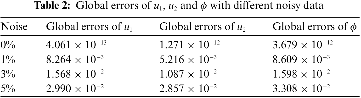
Here are three examples provided to demonstrate the practicality of the current method. The first two examples are derived from a previous study reported by Cao et al. [36], while the third example is based on the work of Xia et al. [29]. The stability of the method is thoroughly examined by introducing the following noise into the input data:

b∼=b(1+rand×δ100),(21)

where b represents the exact data, rand denotes a randomly generated number using the MATLAB function ‘2 * rand − 1’, and δ represents the noise level. The L2 error defined below is utilized:

L2Error=∑i=1Mtotal(Unumericali−Uexacti)2/∑i=1Mtotal(Uexacti)2,(22)

where Mtotal is the number of calculation points. The number of points chosen within each sub-domain is denoted by m=20 and m=40 for 2D and 3D problems, respectively. The impact of m on the accuracy of numerical results can be explored in [21,30].

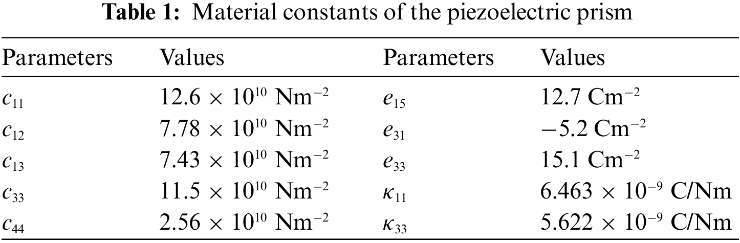
4.1 Test Problem 1: Simple Tension of a Piezoelectric Prism

Firstly, a PZT-4 piezoelectric prism subjected to a simple tension (P=10 Pa) is studied [36]. The structure’s geometry is depicted in Fig. 1. The material constants for the piezoelectric prism, listed in Table 1, are identical to those employed in [36]. The dimensions of the structure are set to be a=3 m and h=10 m. In our computations, the entire domain is discretized into N = 1336 evenly distributed points. The analytical solutions for this problem can be found in [27,36]. In this example, the top surface (z=10) of the structure is chosen as the under-specified boundary.

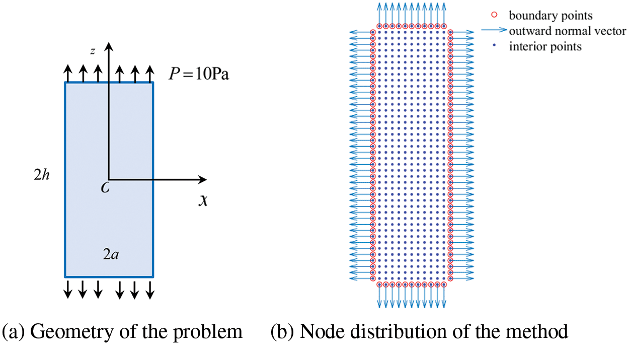
Figure 1: (a) Geometry of the problem and (b) the node distribution of method

Figs. 2a–2c display contour plots showcasing the errors of the electrical potential ϕ at various points within the computational domain. The figures correspond to scenarios with 0%, 0.5%, and 1% noisy data, respectively. Similar results for stresses σzz can be observed in Figs. 3a–3c. Therefore, the current GFDM can provide stable solutions for inverse Cauchy problems.

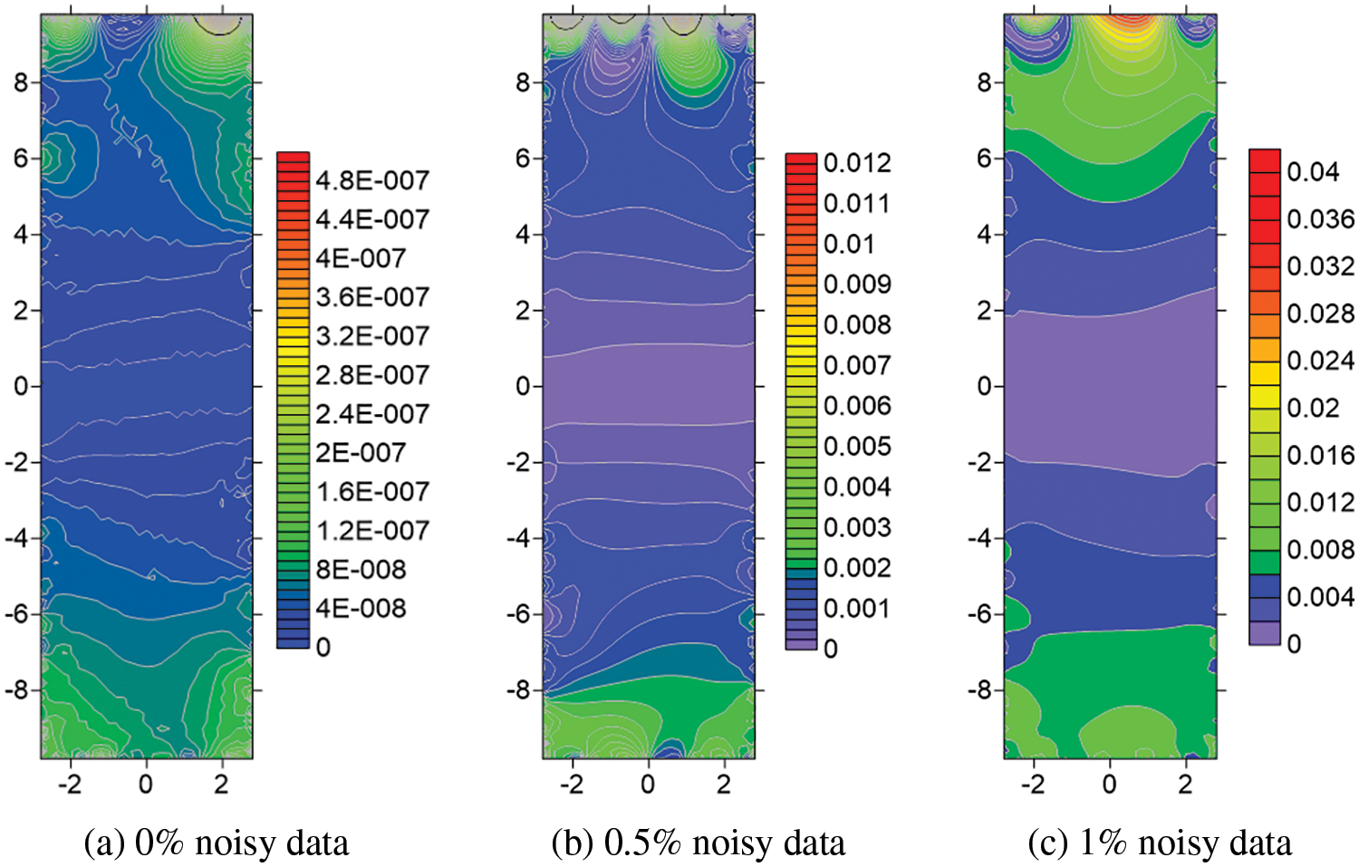
Figure 2: Contour plots of the relative errors of the calculated ϕ at points inside the entire domain with (a) 0% noisy data, (b) 0.5% noisy data, and (c) 1% noisy data

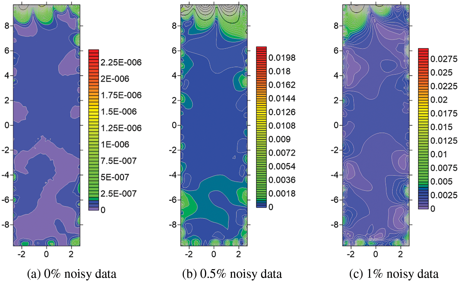
Figure 3: Contour plots of the errors of the calculated σzz with (a) 0% noisy data, (b) 0.5% noisy data, and (c) 1% noisy data

We proceed to examine the sensitivity of the method in relation to m, which denotes the number of collocation points within each local sub-domain. Fig. 4 illustrates the global errors of u2 and ϕ as functions of m, with 1% noisy data. It can be found that the performance of the current method is relatively unaffected by the choice of m. Fig. 5a presents the variation of the condition number of the method against the total number of collocation points, considering 1% noise in the input data. Fig. 5b shows the convergence curve of the calculated electrical potential with respect to the total number of GFDM points, again with 1% noise added to the input data.

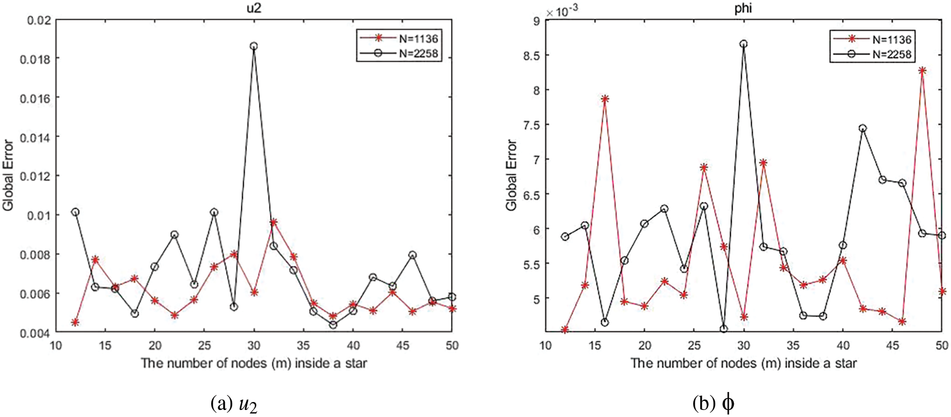
Figure 4: Errors of (a) u2 and (b) ϕ with respect to m, with 1% noisy data

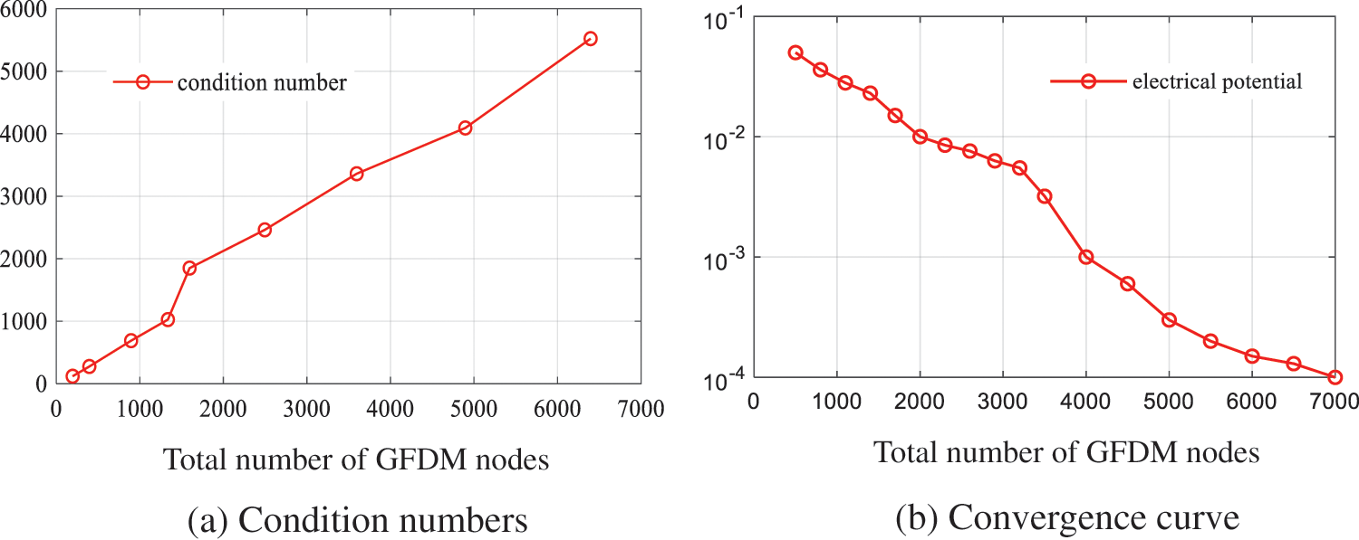
Figure 5: (a) Condition numbers of the current GFDM method and (b) the convergence curve of the electrical potential with 1% noisy data

4.2 Test Problem 2: Bending of a Piezoelectric Panel

As illustrated in Fig. 6, we examine again a piezoelectric strip composed of PZT-4 material (1.0×1.0 mm), with linearly varying stresses specified along the right-side boundary [28,37]. A total of N = 437 evenly distributed points are discretized throughout the entire domain. Here, the top surface of the structure is under-specified.

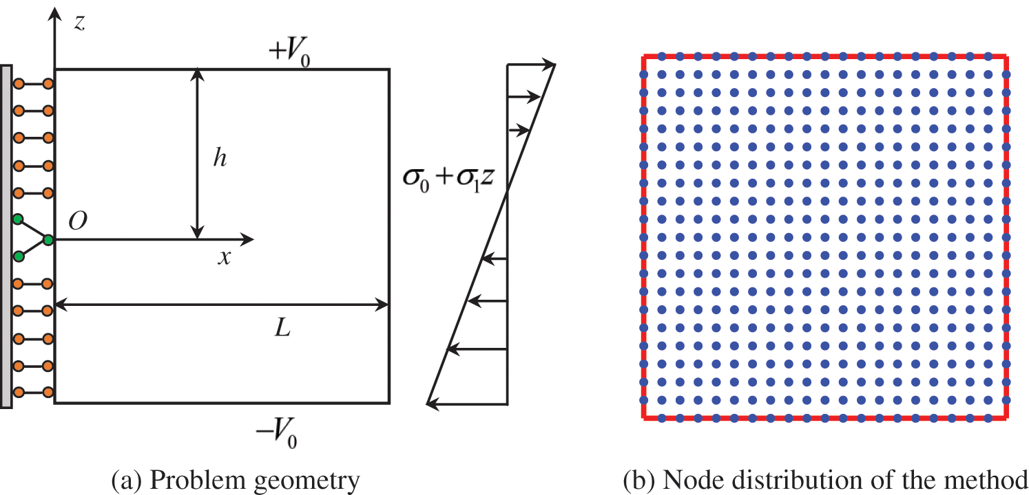
Figure 6: (a) Problem geometry and (b) node distribution of the method

Figs. 7a–7d depict the deformation of the structure with 0%, 1%, 3%, and 5% noisy data, respectively. The background red line represents the original shape. The mechanical deformation obtained throughout the entire domain aligns closely with the results reported in [28,37]. This demonstrates that the present GFDM offers an accurate and stable analysis for this example. Figs. 8a–8d display contour plots illustrating the retrieved displacement (u1) results (dashed lines) across the computational domain, once again considering 0%, 1%, 3%, and 5% noise in the input data. The exact solutions, denoted by solid lines, are provided for comparison purposes. Moreover, as anticipated, the GFDM solution converges towards the exact solution as the level of noise decreases. The global errors of u1, u2 and ϕ, as defined by Eq. (22), are listed in Table 2.

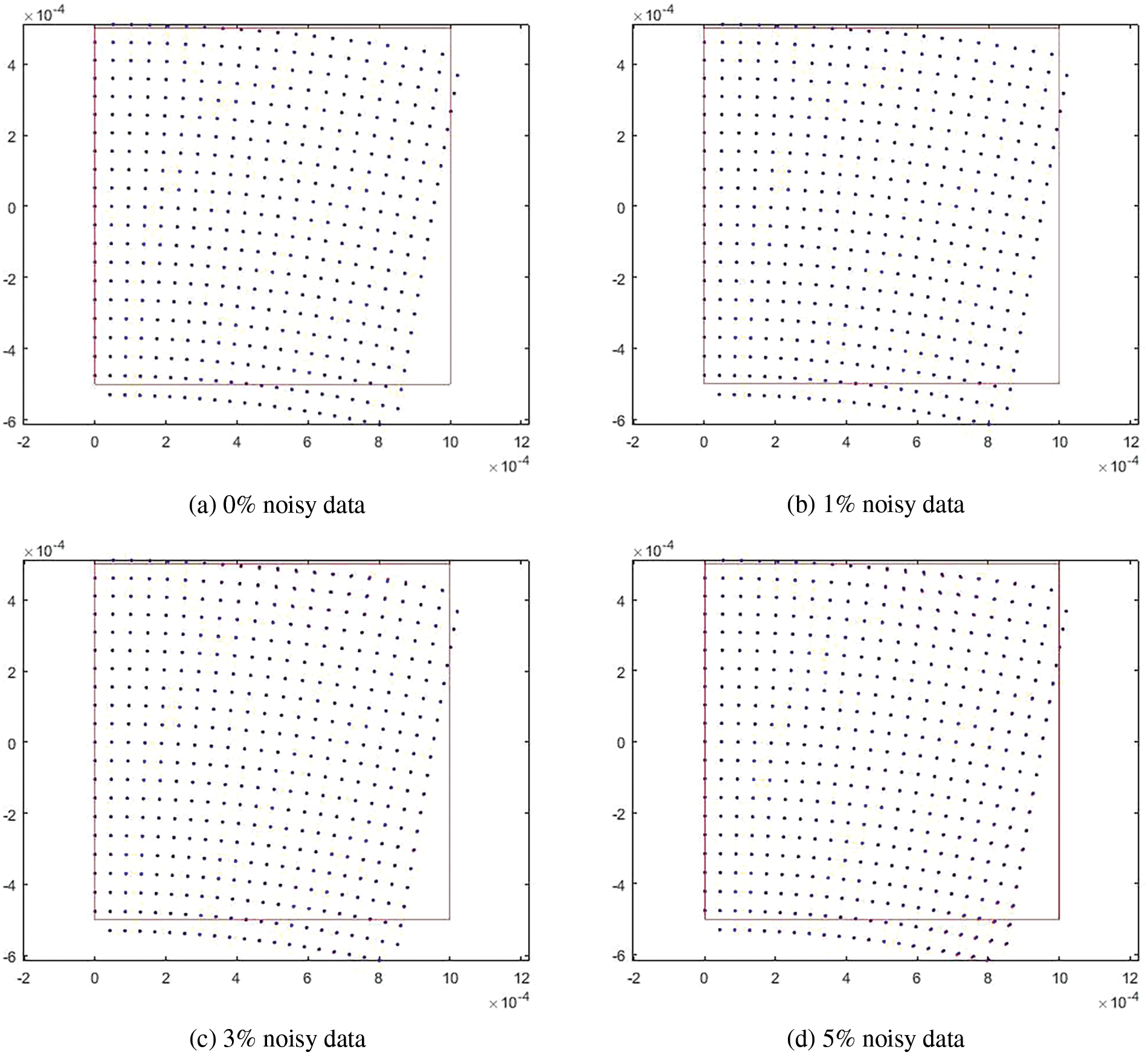
Figure 7: Mechanical deformation of the structure, with (a) 0% noisy data, (b) 1% noisy data, (c) 3% noisy data, and (d) 5% noisy data

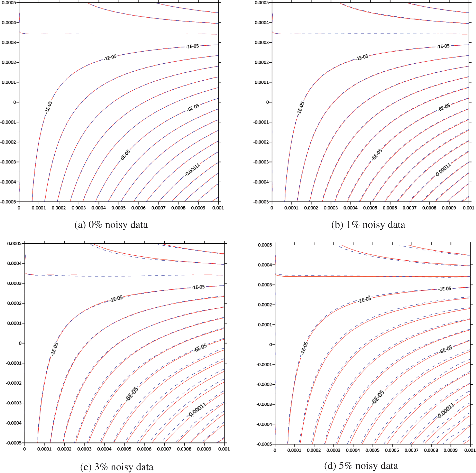
Figure 8: Contour plots of the calculated displacement u1, with (a) 0% noisy data, (b) 1% noisy data, (c) 3% noisy data, and (d) 5% noisy data

4.3 Test Problem 3: A 3D Piezoelectric Column under Uniaxial Tension

In Fig. 9, we examine the inverse electroelastic problem within a 3D cubic domain (1 mm×1 mm×1 mm) subjected to uniaxial tension p=100 N/m2. The material constants of the structure and the corresponding exact solutions can be found in [38]. In our computations, a total of N = 1215 collocation points are discretized throughout the entire domain. Once again, in the context of the inverse Cauchy problem considered here, the top surface of the structure is under-specified due to the unavailability of boundary data.

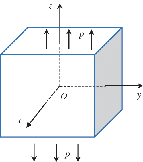
Figure 9: Geometry of the problem

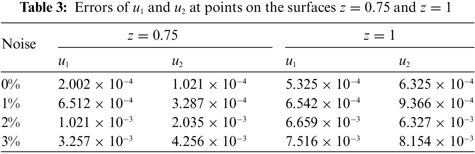
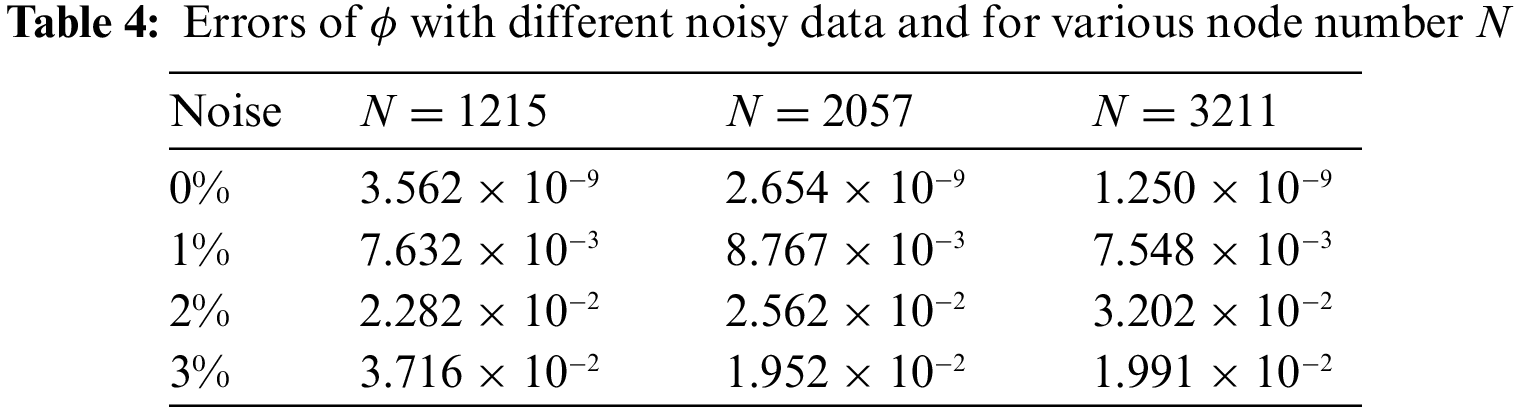
Figs. 10a–10d present contour plots illustrating the retrieved displacements (u1) (dashed lines) at points on the surface z=0.5 for different noisy data. The exact solutions (solid lines) are also provided for comparison. It is evident that the obtained displacement results exhibit excellent agreement with their corresponding analytical solutions, even when 3% noise is present in the input data. In Fig. 11, the calculated displacements u2 at points on the surface z=0.5 are depicted. Similarly, the errors of calculated displacements u1 and u2 at points on the surfaces z=0.75 and z=1 are listed in Table 3. Variations of the errors of the computed electrical potential ϕ with respect to different noisy data and various node numbers N are summarized in Table 4. It is evident that the present numerical results exhibit strong agreement with their corresponding exact solutions across a wide range of noise levels in the input data.

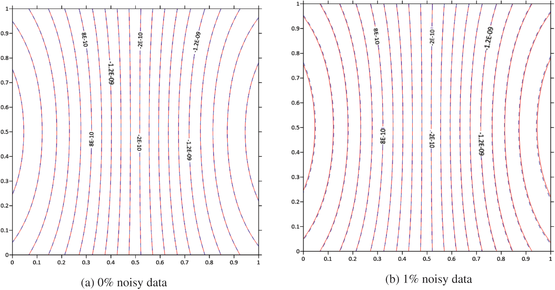
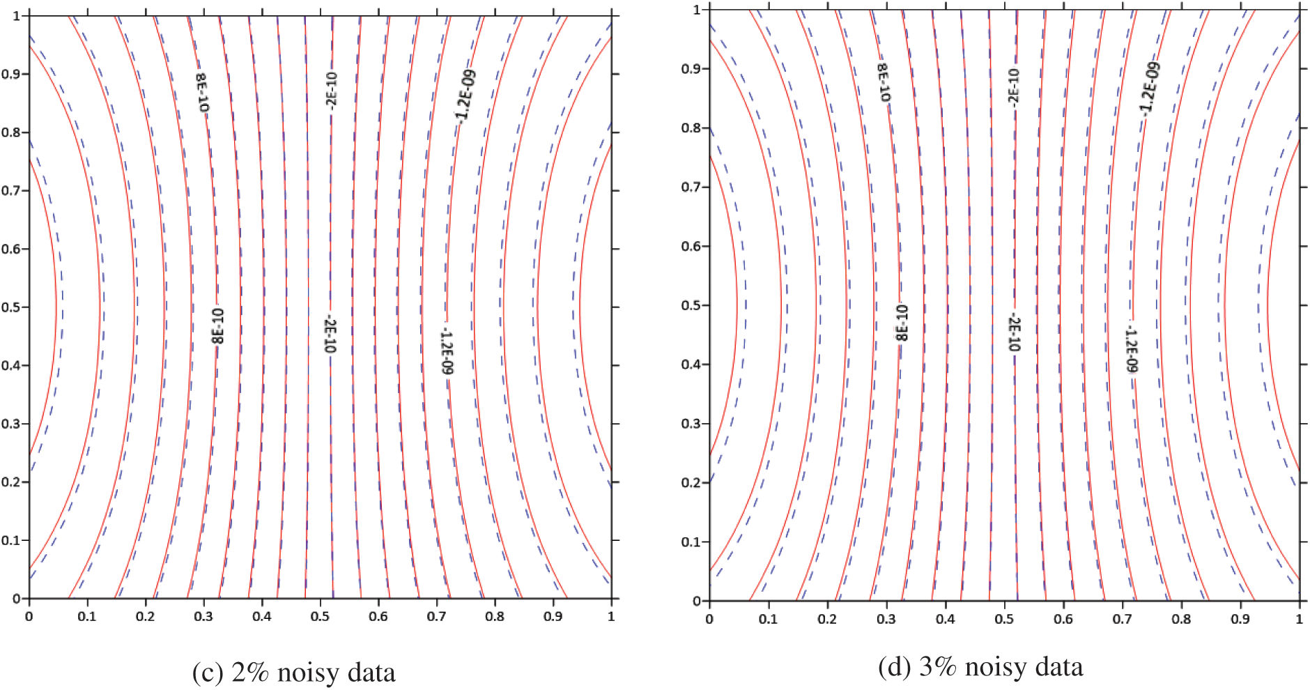
Figure 10: Contour plots of the calculated displacement u1 at the surface z=0.5, with (a) 0% noisy data, (b) 1% noisy data, (c) 2% noisy data, and (d) 3% noisy data

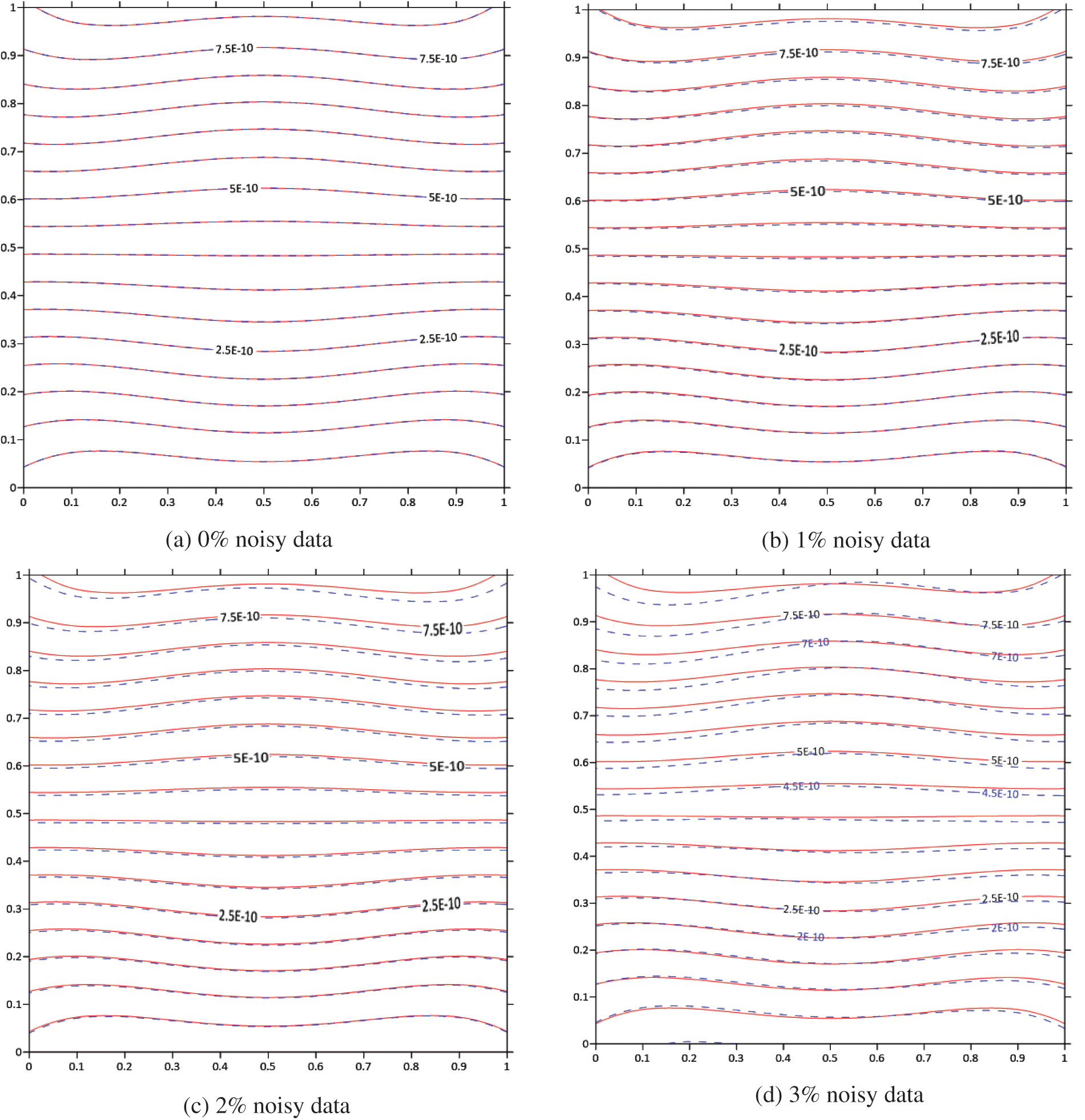
Figure 11: Contour plots of the calculated displacement u2 at the surface z=0.5, with (a) 0% noisy data, (b) 1% noisy data, (c) 2% noisy data, and (d) 3% noisy data

4.4 Test Problem 4: A 3D Solid with Irregular Shape

Finally, we consider a 3D solid with an irregular shape, as shown in Fig. 12. The principal dimension of the solid is 5 m in length, 1.5 m in width, and 5 m in height. A total number of 4650 irregularly distributed GFDM nodes are discretized across the entire domain, where the nodes are generated by using the popular CAE software Hypermesh. The over-specified boundary is taken to be the left-half surface of the boundary, i.e., Γ1={−2.5≤y≤0}. The material constants of the solid and the corresponding exact solutions can be found in [35]. Variations of the errors of the computed u1, u2, u3 and ϕ with respect to different noisy data are summarized in Table 5. It is evident that the present numerical results exhibit strong agreement with their corresponding exact solutions across a wide range of noise levels in the input data.

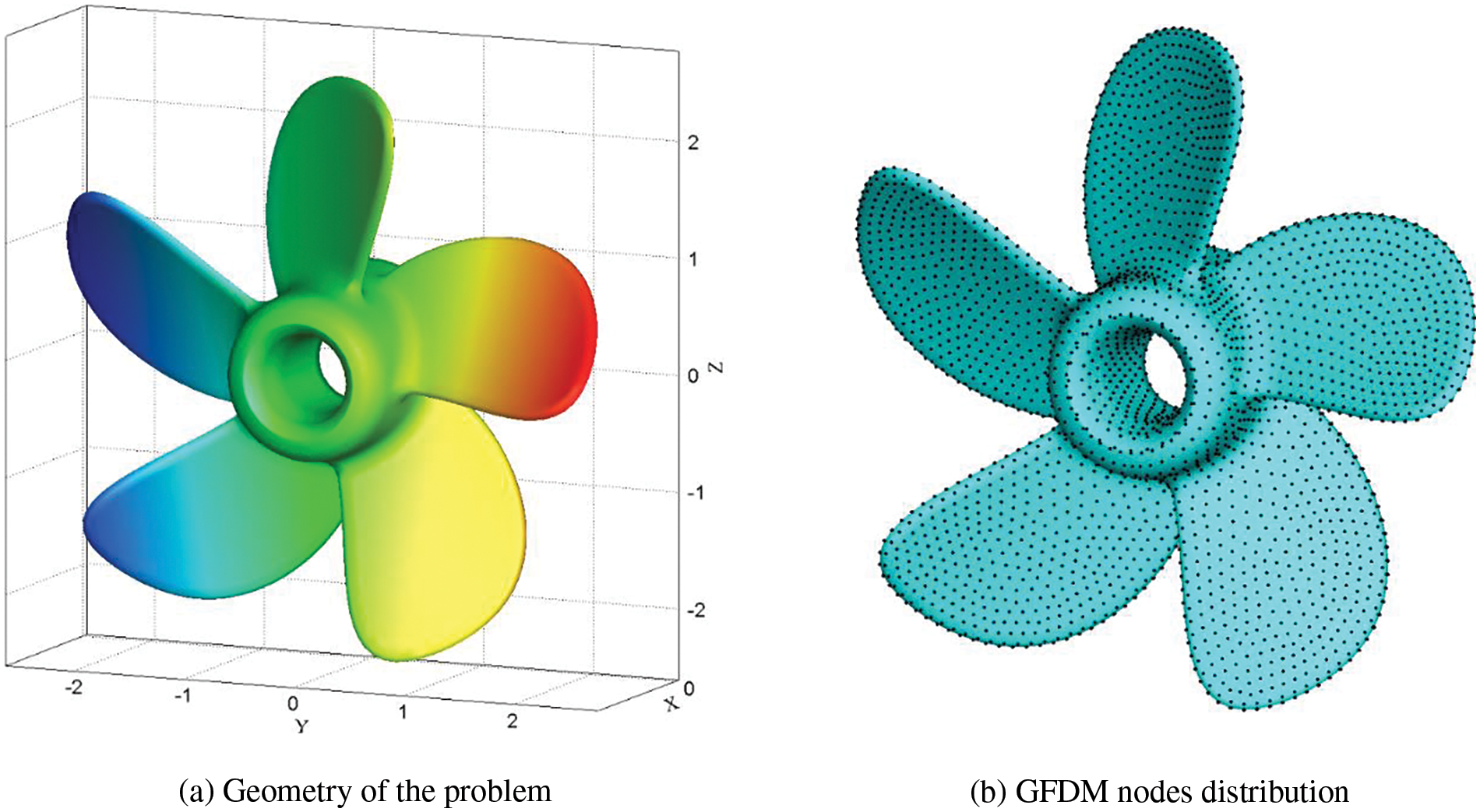
Figure 12: (a) Geometry of the problem and (b) the configuration of the GFDM nodes distribution

5  Conclusions

This study presents the first application of the GFDM for inverse electroelastic analysis in both 2D and 3D piezoelectric structures. The GFDM divides the domain into overlapping small domains and utilizes the Taylor approximation and moving least-squares tool within each local sub-domain to obtain explicit formulas for partial derivatives of PDEs. In inverse Cauchy problems, numerical procedures can become highly unstable, and even small errors in the input data can significantly reduce the overall accuracy of the results. Therefore, we tested the accuracy and stability of the current GFDM by introducing different noisy data into the input data. Our initial numerical experiments demonstrate that the proposed GFDM approach shows great promise for accurately simulating inverse electroelastic problems. Moreover, the method holds the potential for analyzing various other problems, including wave propagation, flow problems, and nonlinear problems. Work in these areas is already underway.

Acknowledgement: The authors would like to acknowledge the valuable feedback provided by the reviewers.

Funding Statement: The research presented in this paper received support from the Natural Science Foundation of Shandong Province of China (Grant No. ZR2022YQ06), the Development Plan of Youth Innovation Team in Colleges and Universities of Shandong Province (Grant No. 2022KJ140), and the Key Laboratory of Road Construction Technology and Equipment (Chang’an University, No. 300102253502).

Author Contributions: The authors confirm contribution to the paper as follows: study conception and design: W.Z. Qu; analysis and interpretation of results: Z.Q. Bai, G.H. Wu; draft manuscript preparation: Z.Q. Bai, W.Z. Qu, G.H. Wu. All authors reviewed the results and approved the final version of the manuscript.

Availability of Data and Materials: No availability of data and materials.

Conflicts of Interest: The authors declare that they have no conflicts of interest to report regarding the present study.

References

1. Lin, J., Liu, C. S. (2022). Recovering temperature-dependent heat conductivity in 2D and 3D domains with homogenization functions as the bases. Engineering with Computers, 38(S3), 2349–2363. [Google Scholar]

2. Jiang, S., Gu, Y., Golub, M. V. (2022). An efficient meshless method for bimaterial interface cracks in 2D thin-layered coating structures. Applied Mathematics Letters, 131, 108080. [Google Scholar]

3. Gu, Y., Sun, L. (2021). Electroelastic analysis of two-dimensional ultrathin layered piezoelectric films by an advanced boundary element method. International Journal for Numerical Methods in Engineering, 122(11), 2653–2671. [Google Scholar]

4. Ju, B., Qu, W. (2023). Three-dimensional application of the meshless generalized finite difference method for solving the extended Fisher–Kolmogorov equation. Applied Mathematics Letters, 136, 108458. [Google Scholar]

5. Qu, W., He, H. (2022). A GFDM with supplementary nodes for thin elastic plate bending analysis under dynamic loading. Applied Mathematics Letters, 124, 107664. [Google Scholar]

6. Gu, Y., Lin, J., Fan, C. M. (2023). Electroelastic analysis of two-dimensional piezoelectric structures by the localized method of fundamental solutions. Advances in Applied Mathematics and Mechanics, 15(4), 880–900. [Google Scholar]

7. Zhao, S., Gu, Y. (2023). A localized Fourier collocation method for solving high-order partial differential equations. Applied Mathematics Letters, 141(5–6), 108615. [Google Scholar]

8. Gu, Y., Fan, C. M., Fu, Z. (2021). Localized method of fundamental solutions for three-dimensional elasticity problems: Theory. Advances in Applied Mathematics and Mechanics, 13(6), 1520–1534. [Google Scholar]

9. Han, Y., Yan, Z., Lin, J., Feng, W. (2022). A novel model and solution on the bending problem of arbitrary shaped magnetoelectroelastic plates based on the modified strain gradient theory. Journal of Intelligent Material Systems and Structures, 33(8), 1072–1086. [Google Scholar]

10. Gu, Y., Fu, Z., Golub, M. V. (2022). A localized Fourier collocation method for 2D and 3D elliptic partial differential equations: Theory and MATLAB code. International Journal of Mechanical System Dynamics, 2(4), 339–351. [Google Scholar]

11. Li, Y., Liu, C., Li, W., Chai, Y. (2023). Numerical investigation of the element-free Galerkin method (EFGM) with appropriate temporal discretization techniques for transient wave propagation problems. Applied Mathematics and Computation, 442, 127755. [Google Scholar]

12. Sun, W., Ma, H., Qu, W. (2023). A hybrid numerical method for non-linear transient heat conduction problems with temperature-dependent thermal conductivity. Applied Mathematics Letters, 124, 108868. https://doi.org/10.1016/j.aml.2023.108868 [Google Scholar] [CrossRef]

13. Qu, W., Fan, C. M., Li, X. (2020). Analysis of an augmented moving least squares approximation and the associated localized method of fundamental solutions. Computers & Mathematics with Applications, 80(1), 13–30. [Google Scholar]

14. Fu, Z., Xi, Q., Gu, Y., Li, J., Qu, W. et al. (2023). Singular boundary method: A review and computer implementation aspects. Engineering Analysis with Boundary Elements, 147(3), 231–266. [Google Scholar]

15. Li, X., Li, S. (2021). A linearized element-free Galerkin method for the complex Ginzburg-Landau equation. Computers & Mathematics with Applications, 90, 135–147. [Google Scholar]

16. Gu, Y., Fan, C. M., Xu, R. P. (2019). Localized method of fundamental solutions for large-scale modeling of two-dimensional elasticity problems. Applied Mathematics Letters, 93(7), 8–14. [Google Scholar]

17. Gu, Y., Lin, J., Wang, F. (2021). Fracture mechanics analysis of bimaterial interface cracks using an enriched method of fundamental solutions: Theory and MATLAB code. Theoretical and Applied Fracture Mechanics, 116(3), 103078. [Google Scholar]

18. Liszka, T., Orkisz, J. (1980). The finite difference method at arbitrary irregular grids and its application in applied mechanics. Computers & Structures, 11(1–2), 83–95. [Google Scholar]

19. Li, P. W., Fan, C. M. (2017). Generalized finite difference method for two-dimensional shallow water equations. Engineering Analysis with Boundary Elements, 80(8), 58–71. [Google Scholar]

20. Fan, C. M., Huang, Y. K., Li, P. W., Chiu, C. L. (2014). Application of the generlized finite-difference method to inverse biharmonic boundary-value problems. Numerical Heat Transfer, Part B: Fundamentals, 65(2), 129–154. [Google Scholar]

21. Gu, Y., Qu, W., Chen, W., Song, L., Zhang, C. (2019). The generalized finite difference method for long-time dynamic modeling of three-dimensional coupled thermoelasticity problems. Journal of Computational Physics, 384, 42–59. [Google Scholar]

22. Jiang, S., Gu, Y., Fan, C. M., Qu, W. (2021). Fracture mechanics analysis of bimaterial interface cracks using the generalized finite difference method. Theoretical and Applied Fracture Mechanics, 113, 102942. [Google Scholar]

23. Gu, Y., Sun, H. (2020). A meshless method for solving three-dimensional time fractional diffusion equation with variable-order derivatives. Applied Mathematical Modelling, 78, 539–549. [Google Scholar]

24. Hu, W., Gu, Y., Zhang, C., He, X. (2019). The generalized finite difference method for an inverse boundary value problem in three-dimensional thermo-elasticity. Advances in Engineering Software, 131(6), 1–11. [Google Scholar]

25. Gong, R., Wang, M., Huang, Q., Zhang, Y. (2023). A CCBM-based generalized GKB iterative regularization algorithm for inverse Cauchy problems. Journal of Computational and Applied Mathematics, 432(1), 115282. [Google Scholar]

26. Zhang, Y. (2022). On the acceleration of optimal regularization algorithms for linear ill-posed inverse problems. Calcolo, 60(1), 6. [Google Scholar]

27. Ding, H. J., Wang, G. Q., Chen, W. Q. (1998). A boundary integral formulation and 2D fundamental solutions for piezoelectric media. Computer Methods in Applied Mechanics and Engineering, 158(1–2), 65–80. [Google Scholar]

28. Xia, H., Gu, Y. (2021). Short communication: The generalized finite difference method for electroelastic analysis of 2D piezoelectric structures. Engineering Analysis with Boundary Elements, 124(2), 82–86. [Google Scholar]

29. Xia, H., Gu, Y. (2021). Generalized finite difference method for electroelastic analysis of three-dimensional piezoelectric structures. Applied Mathematics Letters, 117, 107084. [Google Scholar]

30. Wang, Y., Gu, Y., Fan, C. M., Chen, W., Zhang, C. (2018). Domain-decomposition generalized finite difference method for stress analysis in multi-layered elastic materials. Engineering Analysis with Boundary Elements, 94(33–40), 94–102. [Google Scholar]

31. Ureña, F., Gavete, L., García, A., Benito, J. J., Vargas, A. M. (2019). Solving second order non-linear parabolic PDEs using generalized finite difference method (GFDM). Journal of Computational and Applied Mathematics, 354(4), 221–241. [Google Scholar]

32. Benito, J. J., Ureña, F., Gavete, L. (2001). Influence of several factors in the generalized finite difference method. Applied Mathematical Modelling, 25(12), 1039–1053. [Google Scholar]

33. Wang, K., Li, L., Lan, Y., Dong, P., Xia, G. (2019). Application research of chaotic carrier frequency modulation technology in two-stage matrix converter. Mathematical Problems in Engineering, 2019, 2614327. [Google Scholar]

34. Fan, C. M., Li, P. W., Yeih, W. C. (2015). Generalized finite difference method for solving two-dimensional inverse Cauchy problems. Inverse Problems in Science and Engineering, 23, 737–759. [Google Scholar]

35. Gu, Y., Wang, L., Chen, W., Zhang, C., He, X. (2017). Application of the meshless generalized finite difference method to inverse heat source problems. International Journal of Heat and Mass Transfer, 108(3), 721–729. [Google Scholar]

36. Cao, C., Qin, Q. H., Yu, A. (2012). Hybrid fundamental-solution-based FEM for piezoelectric materials. Computational Mechanics, 50(4), 397–412. [Google Scholar]

37. Ohs, R. R., Aluru, N. R. (2001). Meshless analysis of piezoelectric devices. Computational Mechanics, 27(1), 23–36. [Google Scholar]

38. Ding, H., Liang, J. (1999). The fundamental solutions for transversely isotropic piezoelectricity and boundary element method. Computers & Structures, 71(4), 447–455. [Google Scholar]