Wavelet Multi-Resolution Interpolation Galerkin Method for Linear Singularly Perturbed Boundary Value Problems

1  Introduction

The singularly perturbed boundary value problem originates from fluid mechanics and arises in the mathematical modeling of physical engineering problems. In this study, we consider the following second-order singularly perturbed two-point boundary value problem:

εu″(x)+pu′(x)+qu(x)=f(x),x∈[a,b],u(a)=ua,u(b)=ub(1)

where ε is a small perturbation parameter that satisfies 0<ε≪1, and q is a negative number. A key feature of this problem is the presence of a boundary layer in which the solution undergoes large variations with localized steep gradients as ε approaches zero. We assume that p is a non-zero parameter, and Eq. (1) features a left-side boundary layer at x = a when p>0, and a right-side boundary layer at x = b for p<0.

The presence of boundary layers makes it challenging to solve singularly perturbed problems using classical numerical methods. Consequently, numerous special schemes have been proposed, including transforming the boundary value problem into an initial value problem [1–3], fitting the finite difference method [4], spline method [5–8], finite element method [9–12], and other methods [13–17]. In recent years, algorithms based on layer-adapted meshes have become powerful tools for solving singular perturbation problems [18–20], such as the Shishkin mesh [7,21–23] and Bakhvalov mesh [24–27].

Over recent decades, meshfree methods that rely only on nodes to make approximations have attracted considerable research interest [28–32]. As pointed out by Li et al. [28], meshfree methods are not only complementary to conventional finite element methods, but they also offer several advantages over mesh-based methods. These advantages include the utilization of higher-order continuous shape functions and the elimination of sensitivity to mesh alignment [31,33,34]. Currently, meshfree methods are widely used for solving singularly perturbed boundary value problems because they can quickly obtain more satisfactory numerical solutions by adding extra approximation nodes in the boundary layer. For example, Shen [35] proposed a local radial basis function (RBF)-based differential quadrature collocation method to solve the singularly perturbed two-point boundary value problem, which avoids highly ill-conditioned dense interpolation matrices. Although that study only discussed uniformly distributed nodes, numerical results showed that the local RBF-based collocation method is more accurate and efficient than the globally supported method. The collocation methods are known for being efficient as no integration is required, but they are less stable and accurate. To reduce errors in the standard element-free Galerkin method near the boundary layer, Zhang et al. [36] proposed the variational multiscale element-free Galerkin method to obtain the numerical solutions of convection-diffusion-reaction equations. Numerical results showed that their method is considerably more accurate than the standard element-free Galerkin method, although slight spurious oscillations persisted near the boundary layer. Zhang et al. [37] later presented a novel adaptive algorithm based on the variational multiscale element-free Galerkin method to overcome this drawback. Although many credible results have been obtained using the aforementioned meshfree methods, they still possess some shortages, such as difficulty in imposing of essential boundary conditions and calculating integrals owing to their shape functions are rational functions and lacking the Kronecker delta property [31].

Wavelet-based methods have gained increasing attention as they are widely and successfully used in practical applications [38–42]. Numerical methods based on wavelets can be divided into three main categories: wavelet finite element [39–40,43], wavelet collocation [44–48], and wavelet Galerkin methods [49–53]. Although wavelet finite element methods have advantages over traditional finite element methods, they still suffer from the same disadvantages in the presence of meshes. Existing wavelet meshfree methods do not require meshes, but they do not guarantee accurate interpolations on non-uniform nodes.

Recently, we proposed a truly meshfree method based on wavelet multiresolution analysis, known as the wavelet multiresolution interpolation Galerkin method (WMIGM) [54,55]. Compared with current meshfree methods, WMIGM possesses several advantages [54,55]:

(1)   The proposed wavelet multiresolution interpolation formula possesses the Kronecker delta function property;

(2)   Polynomial reproduction can be achieved up to γ−1 degrees, expressed as linear combinations of shape functions;

(3)   It does not require matrix inversions or ad-hoc parameters;

(4)   The stiffness matrix can be efficiently obtained with an analytical integration method.

A key challenge to solving singularly perturbed boundary value problems is dealing with their singularity, which can lead to numerical instability, oscillations, and spurious solutions [20]. Moreover, the use of uniform nodes in singularly perturbed boundary value problems results in a significant waste of computational effort, as a sufficiently fine mesh is required to accurately capture the rapid variations of the solution near the boundary layer. Therefore, there is a critical need to develop a more efficient, accurate, and stable numerical method specifically designed for solving such problems. The purpose of this study is to employ the WMIGM to solve linear singularly perturbed two-point boundary value problems (see Eq. (1)) based on special segmented equidistant (Shishkin) nodes. A coarse mesh is utilized in the smooth region, and a fine mesh is applied in the boundary layer. Compared with other meshfree methods, our WMIGM approach simplifies the imposition of essential boundary conditions due to its interpolation property. Additionally, we present error estimates of the algorithm, even in the absence of analytic expressions for the shape functions. Test problems are then solved using the WMIGM over modified Shishkin nodes.

This paper is organized as follows. In Section 2, we review the construction of wavelet multiresolution interpolations and some properties of shape functions. In Section 3, we introduce the WMIGM scheme for solving linear singularly perturbed boundary value problems. The parameter uniform convergence is explained in Section 4, followed by numerical experiments and comparisons with existing methods in Section 5, which illustrate the accuracy and efficiency of the proposed wavelet method. Finally, concluding remarks are provided in Section 6.

2  Wavelet Multiresolution Interpolation

This section reviews the construction of the wavelet multiresolution interpolation approximation and explains several key properties of the wavelet interpolating shape function that was proposed in our previous works [54,55].

We begin with the interpolating wavelet transform [44,56], as applied to the following dyadic grids on the real line:

{xj,k∈R:xj,k=a0+2−jkh0,k∈Z},(2)

where xj,k are the grid points, a0 is a real number, j is the decomposition level, and h0 is the spatial step with j = 0. By using the linear superposition of the interpolating wavelet transform, a continuous function f(x)∈L2(R) of the form

f(x)≈PjRf(x)=∑k∈Zf(xj,k)ϕj,kR(x),(3)

is yielded, where ϕj,kR(x)=ϕ0,0R[2j(x−a0)+x0,−k] is the scaling function sampled at point xj,k.

Next, we focus on the interpolating wavelet transform construction for interval [a,b] on a set of dyadic grids:

{xj,k∈[a,b]:xj,k=a+2−jkh0,k=0,1,2,⋯,nj},(4)

where h0=(b−a)/n0 is the spatial step with j = 0, and nj=2jn0 is the number of grids at the level of resolution j, which satisfies n0≥γ.

By applying Eq. (3) to approximate a continuous function f(x)∈L2(R) on the interval [a,b], we obtain

f(x)≈Pj[a,b]f(x)=∑k∈Zf(xj,k)ϕj,kR(x)forx∈[a,b].(5)

Based on the compact support of the scaling function ϕj,kR(x), Eq. (5) can be rewritten as

f(x)≈Pj[a,b]f(x)=∑k=1−γnj+γ−1f(xj,k)ϕj,kR(x).(6)

It can be seen from Eq. (6) that we require the values of f¯(x) at some external auxiliary points located outside the interval [a,b]. Following the work of Donoho [56], the unknown values of f(xj,k) for k<0 or k>nj are obtained with the Lagrange interpolation polynomial of degree γ. It follows that we may define a new function f¯(x) such that

f¯(x)={∑k=0γ−1Lj,ka(x)f(xj,k),x∈[xj,1−γ,a)f(x),x∈[a,b]∑k=nj−γ+1njLj,kb(x)f(xj,k),x∈(b,xj,nj+γ−1],(7)

in which

Lj,ka(x)=∏i=0i≠kγ−1⁡x−xj,ixj,k−xj,i,Lj,kb(x)=∏i=nj−γ+1i≠knj⁡x−xj,ixj,k−xj,i.(8)

Substituting Eq. (7) into Eq. (6), we obtain

Pj[a,b]f(x)=∑k=0njf(xj,k)ϕj,k[a,b](x),(9)

where the modified wavelet scaling function ϕj,k[a,b](x) is given by

ϕj,k[a,b](x)={ϕj,kR(x)+∑i=1−γ−1Lj,ka(xj,i)ϕj,iR(x),k∈[0,γ−1]ϕj,kR(x),k∈[γ,nj−γ]ϕj,kR(x)+∑i=nj+1nj+γ−1Lj,kb(xj,i)ϕj,iR(x),k∈[nj−γ+1,nj].(10)

Lemma 2.1 ([54,56]): The modified scaling function ϕj,k[a,b](x) has the following important properties:

•   Compact support: ϕj,k[a,b](x)=0 for x∉[xj,α,xj,β], where α=max{0,k−γ+1}, β=min{k+γ−1,nj};

•   Interpolation: ϕj,k[a,b](xj,l)=δk,l;

•   Polynomial reproduction: ∑k=0nj(xj,k)iϕj,k[a,b](x)=xi for i=0,1,⋯,γ−1.

Notice that the grid points in Vj[a,b] are regularly spaced. We next introduce multiresolution interpolation [54,55]:

Pj0J,[a,b]f(x)=∑k=0Nf(xk)ΘJ,k[a,b](x),(11)

where N+1 is the total number of nodes in [a,b], and the wavelet multiresolution interpolating shape function ΘJ,k[a,b](x) can be obtained using the following recurrence relation:

ΘJ,k[a,b](x)=ϕk[a,b](x)−∑j=ρ(xk,j0)J−1∑l∈ℳjΘj,k[a,b](xl)ϕl[a,b](x),(12)

with the following initial condition:

Θj1,k[a,b](x)={ϕk[a,b](x),ρ(xk,j0)=j10,ρ(xk,j0)>j1.(13)

In Eq. (13), the function ρ(xk,j0) returns an integer with ρ(xk,j0)≥j0 such that k(x)=2ρ(xk,j0)(x−a)/h0 is an integer. For any point xk, we have xk=xρ(xk,j0),k(xk) and ϕk[a,b](x)=ϕρ(xk,j0),k(xk)[a,b](x). Mj is the set of all nodes xk with ρ(xk,j0)=j+1.

Lemma 2.2 ([54,55]): The wavelet multiresolution interpolating shape function ΘJ,k[a,b](x) has the following important properties:

•   Interpolation: ΘJ,k[a,b](xl)=δk,l;

•   Polynomial reproduction: ∑k=0N(xk)iΘJ,k[a,b](x)=xi for i=0,1,⋯,γ−1.

Definition 2.1: Vj0J,[a,b] is the set of functions f(x) such that every f(x)∈Vj0J,[a,b] has the following representation:

f(x)=∑k=0Nf(xk)ΘJ,k[a,b](x).(14)

Lemma 2.3 ([56]): For function f(x)∈L∞([a,b]), the error between f(x) and Pj0J,[a,b]f(x) can be estimated as

||f(x)−Pj0J,[a,b]f(x)||∞≤C1N−γ,(15)

where C1 is a constant, depending on the derivatives of ΘJ,k[a,b](x) and f(x).

3  Description of the WMIGM

In this section, we formulate the WMIGM for singularly perturbed boundary value problems on Shishkin nodes [19].

3.1 Node Generation

We first divide the computational domain [0,1] into two subintervals each for left- and right-side boundary layer problems: the fine part [0,σ], the crude part [σ,1], and the crude part [0,1−σ], the fine part [1−σ,1], respectively. The transition parameter is defined by σ=min{1/2,αεln⁡(N)/|p|}, where α≥γ, and N∈N is the total number of grids. We consider that the number of grid points in each subdomain is equal and that they are uniformly divided; thus the step of the grid in the rough region is hS=2(1−σ)/N, and that in the fine region is hE=2σ/N. Following the recurrence relation of Eq. (12), we have

hS=2JhE,(16)

in which J is an integer.

In the subsequent calculations, we set σ=1/(2J+1), in which J=max{0,⌈−log2⁡(ε)−α⌉} is an integer, and α is an integer. Thus, we have

ε−1≤2J+α.(17)

We then evenly arrange the nodes into two subintervals:

xk={2−Jkh,if  k=0,1,⋯,N/2σ+(k−N/2)h,   if  k=N/2+1,⋯,N(18)

for left-side boundary layer problems, and

xk={kh,if  k=0,1,⋯,N/2σ+2−Jkh,if  k=N/2+1,⋯,N(19)

for right-side boundary layer problems.

After the nodes are generated, we use the iterative formula in Eq. (12) to obtain the wavelet multiresolution interpolating shape functions. Then, the approximation solution of u(x) can be calculated with Eq. (11).

3.2 WMIGM for Singularly Perturbed Boundary Value Problems

The variational form of Eq. (1) is u(x)∈H01(0,1), such that

−ε∫01u′v′dx+a∫01u′vdx+b∫01uvdx=∫01fvdx  forallv∈H01(0,1).(20)

Then, we replace the infinite dimensional space, H01(0,1), with the wavelet multiresolution interpolation space, Vj0J,[a,b], and obtain the WMIGM:

−ε∫01uh′v′dx+a∫01uh′vdx+b∫01uhvdx=∫01fhvdxforallv∈Vj0J,[0,1],(21)

where uh(x)∈Vj0J,[a,b], and v(x)=ΘJ,l[a,b](x) is selected for l=1,2,3,⋯,N−1.

Using Eq. (11), the approximate solutions for uh(x) and fh(x) can be represented by

{uh(x)=∑k=0Nuh(xk)ΘJ,k[0,1](x)fh(x)=∑k=0Nfh(xk)ΘJ,k[0,1](x).(22)

Substituting Eq. (22) into Eq. (21), we obtain the following matrix form:

−εA0uh+aA1uh+bA2uh=A2fh,(23)

in which the matrices are A0={A0,k1,l=ΓJ,J,k1,lΘ,1,1,[0,1]},A1={A1,k1,l=ΓJ,J,k1,lΘ,0,1,[0,1]}, and A2={A2,k1,l=ΓJ,J,k1,lΘ,0,0,[0,1]}. The vectors are uh={uh,l,1=uh(xl)} and fh={fh,l,1=fh(xl)} for k,l=0,1,2,⋯,N and k1,l1=1,2,3,⋯,N−1, respectively. Here, the connection coefficients, ΓJ,J,k,lΘ,n,m,[0,1]=∫01ΘJ,k(n),[0,1](x)ΘJ,l(m),[0,1](x)dx, can be precisely obtained [54].

Using this process, we can obtain the WMIGM solutions by solving Eq. (23).

4  Error Analysis

In this section, we provide the WMIGM’s error estimate, which relies on the modified Shishkin nodes. In the following analysis, we assume that εN≥21−α to ensure that N≥2J+1 holds. The solution of Eq. (1) can be decomposed into u=S+E, in which S is the smooth component and E is the boundary layer component [12,21,57,58], where

|S(k)(x)|≤C,  |E(k)(x)|≤Cε−ke−βx/εfork=0,1,⋯,γandx∈[0,1].(24)

Based on the properties of the wavelet multiresolution interpolating shape functions introduced in the previous Section 2, we have the following interpolation error estimates.

Lemma 4.1: Let Pj0Ju be the wavelet multiresolution interpolant of u(x) on the modified Shishkin nodes. Thus, we obtain the properties for

||u−Pj0Ju||L∞(Ω)≤CN−γ,(25)

||u−Pj0Ju||ε≤CN1−γ,(26)

where C is independent of N and ε, and the energy norm is defined as

||v||ε:={ε||v′||L22−q||v||L22}1/2  ∀v∈H1(Ω).(27)

Proof: Using a Taylor expansion at xi, the interpolation error of |S(x)−Pj0J,[a,b]S(x)| for x∈[xi,xi+1] can be rewritten as

|S(x)−Pj0JS(x)|=S(γ)(ς)γ!(x−xi)γ,(28)

where ς∈[xi,x]. From Eq. (24), we get

|S(x)−Pj0JS(x)|≤ChSγ≤CN−γ.(29)

Then, from Eqs. (17) and (24), on the boundary layer part, we have

|E−Pj0JE(x)|=E(γ)(ς)γ!(x−xi)γ≤ChEγε−γ≤CN−γ(22J+1ε−1)γ≤CN−γ(2J+α+12J+1)γ.≤CN−γ(30)

Obviously, Eq. (25) can be easily demonstrated through Eqs. (28) and (30).

Thus, it remains to prove the estimate Eq. (26). From Eq. (24), we get

||(u−Pj0Ju)′||L2(ΩS)≤ChSγ−1||E(k)(x)||L2(ΩS)≤ChSγ−1(1−σ),≤ChSγ−1≤CN1−γ(31)

||(u−Pj0Ju)′||L2(ΩE)≤ChEγ−1||E(k)(x)||L2(ΩE)≤ChEγ−1(σε−2γ)1/2.≤ChEγ−1(2αε1−2γ)1/2≤Cε−1/2N1−γ(32)

The estimation of Eq. (26) can then be derived immediately.

Theorem 4.1: Let u be the solution of Eq. (1) and uN∈Vj0J,[a,b] be the WMIGM solution of Eq. (23). Thus, we have

||u−uN||ε≤CN1−γ,forNε≥21−α,(33)

in which C is independent of N and ε.

Proof: Let ξ:=Pj0Ju−uN. Applying the Galerkin orthogonality, we get

||ξ||ε2=ε||(ξ)′||L2(Ω)2−q||ξ||L2(Ω)2=ε|∫01ξ′ξ′dx|−q|∫01ξξdx|.≤ε|∫01(Pj0Ju−u)′ξ′dx|+|−p∫01(Pj0Ju−u)′ξdx|−q|∫01(Pj0Ju−u)ξdx|=:I+II+III(34)

Owing to the Hölder inequalities and Eq. (26) of Lemma 4.1, it holds that

I+III≤C||Pj0Ju−u||ε||ξ||ε≤CN1−γ||ξ||ε.(35)

With the aid of integrating by parts and the Cauchy-Schwarz inequality, we observe that

II=−p∫01(Pj0Ju−u)′ξdx=p∫01(Pj0Ju−u)ξ′dx≤C||u−Pj0Ju||L2(Ω)||ξ||L2(Ω)≤CN−γ||ξ||L2(Ω).≤CN−γ||ξ||ε(36)

As a result,

||ξ||ε≤CN1−γ.(37)

Hence, u−uN can be bounded by

||u−uN||ε≤||u−Pj0Ju||ε+||Pj0Ju−uN||ε≤CN1−γ,(38)

which is the required result.

5  Numerical Results

In this section, we applied the WMIGM to four examples to evaluate its numerical accuracy. We considered two grid points: uniform node points using the wavelet interpolation Galerkin method (WIGM) and refined local grid points using the WMIGM, as specified in Section 3. If not otherwise specified, γ=6 and α=3.

To estimate the accuracy of the solutions, the maximum absolute and ε-uniform errors at the grid points are taken as

Emax(N)=max0≤i≤N|ue(xi)−uh(xi)|Eε(N)={∑i=0Nε[ue′(xi)−uh′(xi)]2−q[ue(xi)−uh(xi)]2}1/2,(39)

and the numerical rates of convergence are

R=log2⁡[Emax,ε(N)/Emax,ε(2N)].(40)

All numerical results were conducted on an AMD Ryzen 7 3700X CPU @ 3.20 GHz with 64 GB RAM in MATLAB.

5.1 Test Problem 1: Left-Side Boundary Layer Problem

We begin our numerical cases with the following left-side boundary layer problem [6–7,59,60]:

εu″+u′=1+2x.(41)

The boundary conditions are extracted from the exact solution as

u(x)=x(x+1−2ε)+(2ε−1)(1−e−x/ε)/(1−e−1/ε).(42)

The absolute errors obtained by the proposed WIGM with N = 100 for different values of ε are presented in Fig. 1. The numerical results show that the errors are mainly located near the left-side boundary layer, and they increase with the decrease of ε. In Table 1, we list the maximum absolute errors and computational orders of convergence on uniform points using the WIGM and non-uniform points using the WMIGM for different values of ε and grid points N with γ=6. From Table 1, we find that the numerical solutions obtained by the WMIGM are much better than those computed by the WIGM, especially for ε→0. In particular, WMIGM using 256 grid points exhibits slightly better accuracy than the WIGM using 512 nodes for ε=2−5 and ε=2−6. Therefore, solution accuracy can be improved by adding local nodes in the boundary layer. Moreover, a comparison of the numerical errors obtained by the WIGM, the WMIGM, the quintic B-spline method (QBSM) with Shishkin mesh [6], and the novel optimal B-spline (NOBS) technique with Shishkin mesh [7] is also illustrated in Table 1. There, it can be seen that for most cases, the WMIGM is more accurate than the QBSM and the NOBS, given the same number of grid points for most cases listed. The numerical solutions obtained by the WIGM and the WMIGM are shown in Fig. 2 with the corresponding exact solution for ε=2−9. Note that the WMIGM with N = 64 can achieve nearly the same accuracy as the analytical solution, whereas the WIGM does not converge at small ε values. To visualize the convergence ratio of the proposed algorithm, Fig. 3 displays the error norm as a function of the number of grid points with ε=2−7. It can be seen that the proposed WMIGM’s convergence rate of Eε(N) is approximately γ−1 for Nε≥2−2, which is consistent with the previous error analysis. Moreover, the curves visually demonstrate that our results are better than the QBSM and the NOBS, and the numerical convergence rate of the maximum error Emax is approximately γ. Notably, the results of the WMIGM with γ=6 are quite bad for N = 32, as shown in Table 1. We conclude that is due to the support domains of the shape functions will become larger as γ increases. Thus, we need more sampling points to capture the local large gradient information for a large γ. We can see that this phenomenon does not occur when γ=4.

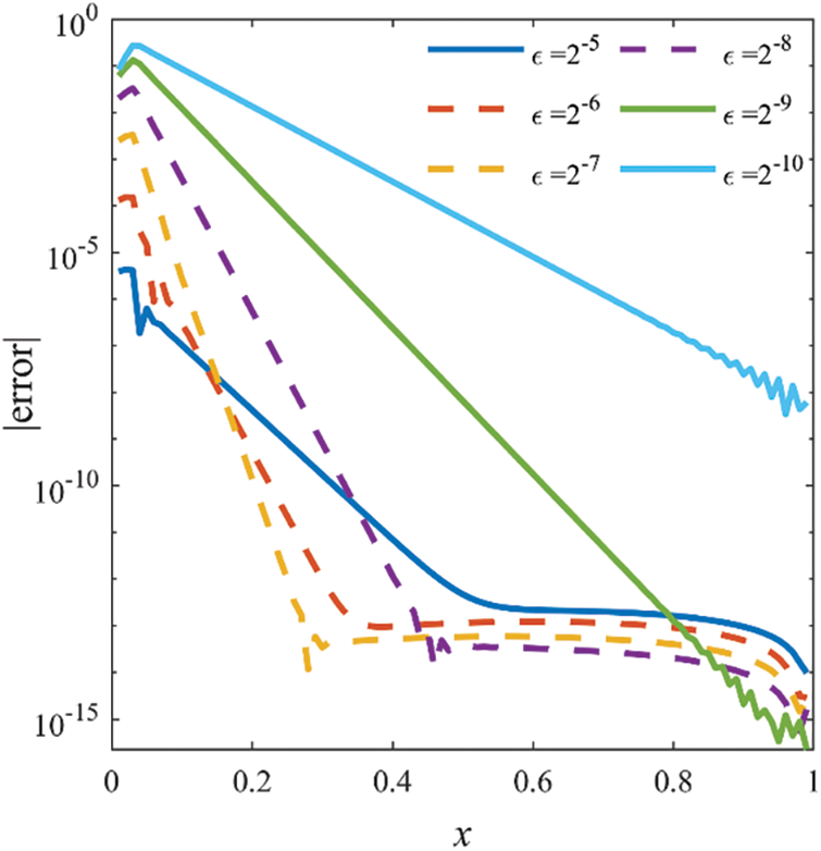
Figure 1: Absolute errors of WIGM for Example 1 with N = 100

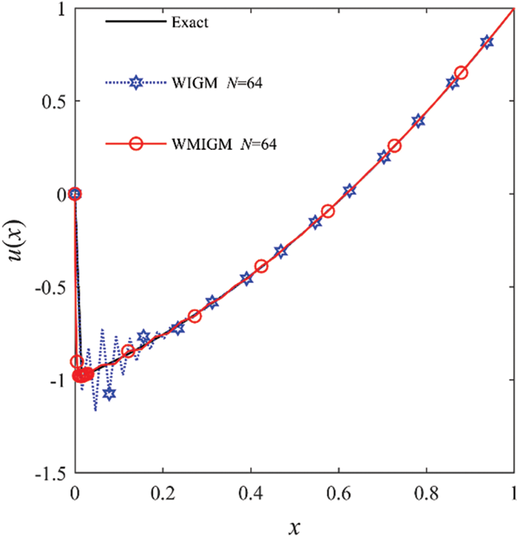
Figure 2: The comparison of the numerical solutions with the exact solution for Example 1 with ε=2−9

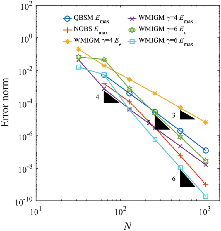
Figure 3: Error norm as a function of the number of grid points for Example 1 with ε=2−7

5.2 Test Problem 2: Left-Side Boundary Layer Problem

We next consider a source-free singularly perturbed problem as described in [3,10,60–62]:

εu″+u′−u=0,(43)

whose analytical solution is given by

u(x)=(em2−1)em1x+(1−em1)em2xem2−em1,(44)

in which m1=(−1+1+4ε)/(2ε) and m2=(−1−1+4ε)/(2ε). The solution u(x) satisfies the boundary conditions of u(0)=1 and u(1)=1.

Table 2 shows the comparison of the maximum absolute errors between the QBSM with Shishkin mesh [6], the NOBS with Shishkin mesh [7], and the proposed WIGM and WMIGM with respect to the number of grid points for various values of ε. It can be seen that the number of grid points must be increased to obtain a reliable numerical solution as ε decreases. We can see from Fig. 4 that the method of locally enhancing nodes at the boundary layer using the WMIGM performs significantly better than the method utilizing uniform nodes using the WIGM when the same number of nodes is used. The latter has obvious spurious oscillations in the boundary layer region. The error norms as a function of the number of nodes are illustrated in Fig. 5, where ε=2−7. We have shown that the WMIGM is much more accurate than the QBSM [6] and the NOBS [7], and the order of accuracy of the WMIGM with ε-uniform error norm is approximately γ−1. Additionally, the maximum absolute error convergence rate of the WMIGM with γ=6 is approximately 6.18, which is larger than that of other algorithms.

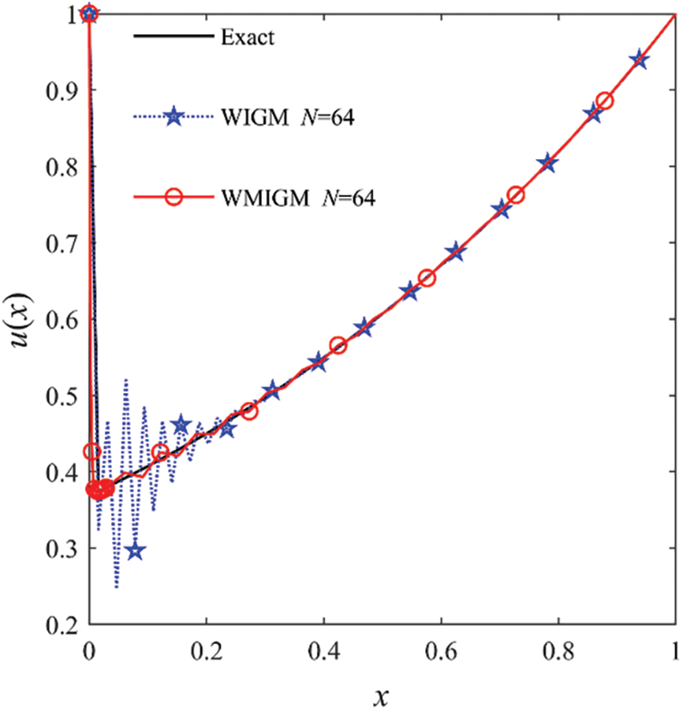
Figure 4: The comparison of the numerical solutions with the exact solution for Example 2 with ε=2−9

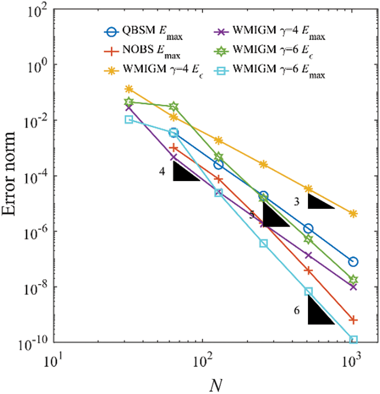
Figure 5: Error norm as a function of the number of grid points for Example 2 with ε=2−7

5.3 Test Problem 3: Right-Side Boundary Layer Problem

We next consider the right-side boundary layer problem [6,13,63–65]:

εu″−u′=0,(45)

with boundary conditions of u(0)=1 and u(1)=0. The exact solution of this problem is

u(x)=e(x−1)/ε−1e−1/ε−1.(46)

Fig. 6 displays the absolute errors for the uniform mesh with different values of ε, and we observe that the errors are mainly located in the right-side boundary layer region. The obtained maximum absolute errors and computational orders of convergence are presented in comparison with the existing QBSM method [6] in Table 3 for different values of ε and N. From this table, we can conclude that our numerical solutions obtained by the WMIGM are in good agreement with the exact values and are more accurate than the QBSM, which is a fourth-order scheme [6]. It can also be seen from Fig. 7 that the non-physical oscillation can be greatly reduced by locally increasing the number of nodes in the boundary layer.

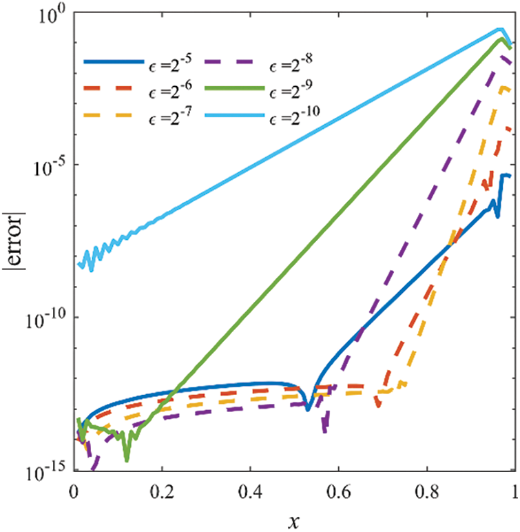
Figure 6: Absolute errors of WIGM for Example 3 with N = 100

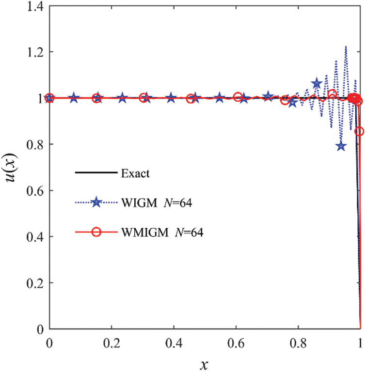
Figure 7: The comparison of the numerical solutions with the exact solution for Example 3 with ε=2−9

5.4 Test Problem 4: Right-Side Boundary Layer Problem

Finally, we consider the following homogeneous linear singularly perturbed boundary value problem [5,7,63,66,67]:

εu″−u′−(1+ε)u=0,(47)

with boundary conditions extracted from the exact solution as

u(x)=e(1+ε)(x−1)/ε+e−x.(48)

The maximum absolute errors obtained by the QBSM with Shishkin mesh [6], the NOBS with Shishkin mesh [7], and the proposed WIGM and WMIGM are presented in Table 4. It is evident from this table that WMIGM can achieve more accurate approximate solutions. A comparison of the numerical and analytic solutions with ε=2−9 is shown in Fig. 8. The accuracy of the present wavelet solution near the right-side boundary layer was improved with the addition of local nodes. Fig. 9 shows that the convergence rate of the proposed WMIGM with γ=6 is 6.19, whereas the convergence orders of the QBSM with Shishkin mesh [6] and the NOBS with Shishkin mesh [7] are only 3.81 and 4.89, respectively. Therefore, the WMIGM is significantly more accurate than these previously developed methods.

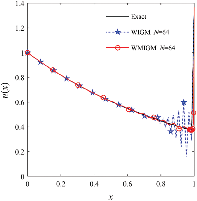
Figure 8: The comparison of the numerical solutions with the exact solution for Example 4 with ε=2−9

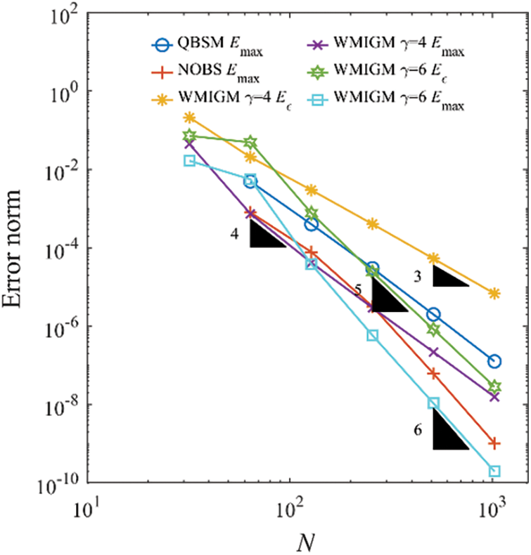
Figure 9: Error norm as a function of the number of grid points for Example 4 with ε=2−7

6  Conclusion

In this study, we extended the WMIGM to solve linear singularly perturbed boundary value problems with modified Shishkin nodes. The proposed wavelet scheme was verified by comparing the numerical solutions obtained via the QBSM with Shishkin mesh and the NOBS with Shishkin mesh. The numerical results confirm the theoretical analysis and demonstrate that WMIGM has several advantages over existing schemes:

(1)   The accuracy of the WMIGM is significantly better than that of the WIGM. The approximate solutions obtained by the WMIGM exhibit no obvious spurious oscillations near the boundary layer, even as the perturbation parameter approaches zero.

(2)   The WMIGM exhibits greater accuracy than existing schemes, including those of the QBSM and NOBS methods with Shishkin mesh.

(3)   The WMIGM demonstrates a six-order convergence rate and retains a stable convergence order better than that of the QBSM and NOBS methods with the Shishkin mesh.

These advantages indicate the potentially wide application of the WMIGM to simulating problems with local large gradients. Since the proposed WMIGM allows a very flexible nodal distribution, it can be extended to solve other problems with localized steep gradients, such as the steady-state convection diffusion problems, the steady-state heat transfer at high Péclet numbers, and the planar thin plate problems in solid mechanics. Additionally, the combination of the time integral format and the proposed method enables the solution of time dependent systems, including the Navier-Stokes equations with large Reynolds numbers and convective heat transfer problems with large Péclet numbers. Moreover, combining WMIGM with wavelet adaptive analysis holds great appeal as a potentially superior method for solving these intricate problems.

Acknowledgement: The authors sincerely thanks the reviewers and the editors of the journal for the great improvement of this paper.

Funding Statement: This work was supported by the National Natural Science Foundation of China (No. 12172154), the 111 Project (No. B14044), the Natural Science Foundation of Gansu Province (No. 23JRRA1035), and the Natural Science Foundation of Anhui University of Finance and Economics (No. ACKYC20043).

Author Contributions: The authors confirm contribution to the paper as follows: study conception and design: Jiaqun Wang, Xiaojing Liu; coding: Jiaqun Wang, Guanxu Pan; analysis and interpretation of results: Guanxu Pan, Xiaojing Liu; funding support: Jiaqun Wang, Youhe Zhou, Xiaojing Liu; draft manuscript preparation: Jiaqun Wang, Guanxu Pan; draft review: Youhe Zhou, Xiaojing Liu. All authors reviewed the results and approved the final version of the manuscript.

Availability of Data and Materials: The data that support the findings of this study are available from the corresponding author upon reasonable request.

Conflicts of Interest: The authors declare that they have no conflicts of interest to report regarding the present study.

References

1. Kadalbajoo, M. K., Kumar, D. (2008). A non-linear single step explicit scheme for non-linear two-point singularly perturbed boundary value problems via initial value technique. Applied Mathematics and Computation, 202(2), 738–746. https://doi.org/10.1016/j.amc.2008.03.015 [Google Scholar] [CrossRef]

2. Geng, F. Z., Tang, Z. Q. (2016). Piecewise shooting reproducing kernel method for linear singularly perturbed boundary value problems. Applied Mathematics Letters, 62, 1–8. https://doi.org/10.1016/j.aml.2016.06.009 [Google Scholar] [CrossRef]

3. Liu, C. S., Chang, C. W. (2022). Modified asymptotic solutions for second-order nonlinear singularly perturbed boundary value problems. Mathematics and Computers in Simulation, 193, 139–152. https://doi.org/10.1016/j.matcom.2021.10.005 [Google Scholar] [CrossRef]

4. Reddy, N. R., Mohapatra, J. (2015). An efficient numerical method for singularly perturbed two point boundary value problems exhibiting boundary layers. National Academy Science Letters, 38(4), 355–359. https://doi.org/10.1007/s40009-015-0350-z [Google Scholar] [CrossRef]

5. Kadalbajoo, M. K., Arora, P. (2010). B-splines with artificial viscosity for solving singularly perturbed boundary value problems. Mathematical and Computer Modelling, 52(5–6), 654–666. https://doi.org/10.1016/j.mcm.2010.04.012 [Google Scholar] [CrossRef]

6. Lodhi, R. K., Mishra, H. K. (2017). Quintic B-spline method for solving second order linear and nonlinear singularly perturbed two-point boundary value problems. Journal of Computational and Applied Mathematics, 319, 170–187. https://doi.org/10.1016/j.cam.2017.01.011 [Google Scholar] [CrossRef]

7. Thula, K. (2020). A sixth-order numerical method based on shishkin mesh for singularly perturbed boundary value problems. Iranian Journal of Science and Technology, Transactions A: Science, 46, 161–171. https://doi.org/10.1007/s40995-020-00952-x [Google Scholar] [CrossRef]

8. Lodhi, R. K., Mishra, H. K. (2018). Septic B-spline method for second order self-adjoint singularly perturbed boundary-value problems. Ain Shams Engineering Journal, 9(4), 2153–2161. https://doi.org/10.1016/j.asej.2016.09.016 [Google Scholar] [CrossRef]

9. Zhu, P., Xie, S. L. (2014). Higher order uniformly convergent continuous/discontinuous Galerkin methods for singularly perturbed problems of convection-diffusion type. Applied Numerical Mathematics, 76, 48–59. https://doi.org/10.1016/j.apnum.2013.10.001 [Google Scholar] [CrossRef]

10. Kaushik, A., Vashishth, A. K., Kumar, V., Sharma, M. (2019). A modified graded mesh and higher order finite element approximation for singular perturbation problems. Journal of Computational Physics, 395, 275–285. https://doi.org/10.1016/j.jcp.2019.04.073 [Google Scholar] [CrossRef]

11. Ma, G. L., Stynes, M. (2020). A direct discontinuous Galerkin finite element method for convection-dominated two-point boundary value problems. Numerical Algorithms, 83(2), 741–765. https://doi.org/10.1007/s11075-019-00701-1 [Google Scholar] [CrossRef]

12. Zhang, J., Ma, X. Q., Lv, Y. H. (2021). Finite element method on Shishkin mesh for a singularly perturbed problem with an interior layer. Applied Mathematics Letters, 121, 107509. https://doi.org/10.1016/j.aml.2021.107509 [Google Scholar] [CrossRef]

13. Reddy, J. N., Martinez, M. (2021). A dual mesh finite domain method for steady-state convection-diffusion problems. Computers & Fluids, 214, 104760. https://doi.org/10.1016/j.compfluid.2020.104760 [Google Scholar] [CrossRef]

14. Lin, B., Li, K., Cheng, Z. (2009). B-spline solution of a singularly perturbed boundary value problem arising in biology. Chaos, Solitons & Fractals, 42(5), 2934–2948. https://doi.org/10.1016/j.chaos.2009.04.036 [Google Scholar] [CrossRef]

15. Vulanovic, R., Nhan, T. A. (2021). An improved Kellogg-Tsan solution decomposition in numerical methods for singularly perturbed convection-diffusion problems. Applied Numerical Mathematics, 170, 128–145. https://doi.org/10.1016/j.apnum.2021.07.019 [Google Scholar] [CrossRef]

16. Das, P., Natesan, S. (2013). Richardson extrapolation method for singularly perturbed convection-diffusion problems on adaptively generated mesh. Computer Modeling in Engineering & Sciences, 90(6), 463–485. https://doi.org/10.3970/cmes.2013.090.463 [Google Scholar] [CrossRef]

17. Kadalbajoo, M. K., Gupta, V. (2010). A brief survey on numerical methods for solving singularly perturbed problems. Applied Mathematics and Computation, 217(8), 3641–3716. https://doi.org/10.1016/j.amc.2010.09.059 [Google Scholar] [CrossRef]

18. Kadalbajoo, M. K., Patidar, K. C. (2002). A survey of numerical techniques for solving singularly perturbed ordinary differential equations. Applied Mathematics and Computation, 130(2), 457–510. https://doi.org/10.1016/S0096-3003(01)00112-6 [Google Scholar] [CrossRef]

19. Linß, T. (2003). Layer-adapted meshes for convection–diffusion problems. Computer Methods in Applied Mechanics and Engineering, 192(9–10), 1061–1105. https://doi.org/10.1016/s0045-7825(02)00630-8 [Google Scholar] [CrossRef]

20. Stynes, M. (2005). Steady-state convection-diffusion problems. Acta Numerica, 14, 445–508. https://doi.org/10.1017/S0962492904000261 [Google Scholar] [CrossRef]

21. Zhu, P., Xie, S. L. (2020). A uniformly convergent weak galerkin finite element method on shishkin mesh for 1d convection-diffusion problem. Journal of Scientific Computing, 85(2), 34. https://doi.org/10.1007/s10915-020-01345-3 [Google Scholar] [CrossRef]

22. Wang, Y., Meng, X. Y., Li, Y. H. (2021). The finite volume element method on the Shishkin mesh for a singularly perturbed reaction-diffusion problem. Computers & Mathematics with Applications, 84, 112–127. https://doi.org/10.1016/j.camwa.2020.12.011 [Google Scholar] [CrossRef]

23. Lv, Y. H., Zhang, J. (2022). Convergence and supercloseness of a finite element method for a two-parameter singularly perturbed problem on Shishkin triangular mesh. Applied Mathematics and Computation, 416, 126753. https://doi.org/10.1016/j.amc.2021.126753 [Google Scholar] [CrossRef]

24. Zhang, J., Liu, X. W. (2020). Convergence of a finite element method on a Bakhvalov-type mesh for singularly perturbed reaction-diffusion equation. Applied Mathematics and Computation, 385, 125403. https://doi.org/10.1016/j.amc.2020.125403 [Google Scholar] [CrossRef]

25. Zhang, J., Lv, Y. H. (2021). High-order finite element method on a Bakhvalov-type mesh for a singularly perturbed convection-diffusion problem with two parameters. Applied Mathematics and Computation, 397, 125953. https://doi.org/10.1016/j.amc.2021.125953 [Google Scholar] [CrossRef]

26. Zhang, J., Lv, Y. H. (2021). Finite element method for singularly perturbed problems with two parameters on a Bakhvalov-type mesh in 2D. Numerical Algorithms, 90, 447–475. https://doi.org/10.1007/s11075-021-01194-7 [Google Scholar] [CrossRef]

27. Zhang, J., Lv, Y. (2022). Supercloseness of finite element method on a Bakhvalov-type mesh for a singularly perturbed problem with two parameters. Applied Numerical Mathematics, 171, 329–352. https://doi.org/10.1016/j.apnum.2021.09.010 [Google Scholar] [CrossRef]

28. Li, S., Liu, W. K. (1996). Moving least-square reproducing kernel method Part II: Fourier analysis. Computer Methods in Applied Mechanics and Engineering, 139(1), 159–193. https://doi.org/10.1016/S0045-7825(96)01082-1 [Google Scholar] [CrossRef]

29. Golbabai, A., Kalarestaghi, N. (2018). Improved localized radial basis functions with fitting factor for dominated convection-diffusion differential equations. Engineering Analysis with Boundary Elements, 92, 124–135. https://doi.org/10.1016/j.enganabound.2017.10.008 [Google Scholar] [CrossRef]

30. Wang, J. F., Wu, Y., Xu, Y., Sun, F. X. (2023). A dimension-splitting variational multiscale element-free galerkin method for three-dimensional singularly perturbed convection-diffusion problems. Computer Modeling in Engineering & Sciences, 135(1), 341–356. https://doi.org/10.32604/cmes.2022.023140 [Google Scholar] [CrossRef]

31. Nguyen, V. P., Rabczuk, T., Bordas, S., Duflot, M. (2008). Meshless methods: A review and computer implementation aspects. Mathematics and Computers in Simulation, 79(3), 763–813. https://doi.org/10.1016/j.matcom.2008.01.003 [Google Scholar] [CrossRef]

32. Liu, G. R. (2009). Meshfree methods: Moving beyond the finite element method, 2nd ed. Boca Raton: CRC Press. [Google Scholar]

33. Tayebi, A., Shekari, Y., Heydari, M. H. (2017). A meshless method for solving two-dimensional variable-order time fractional advection-diffusion equation. Journal of Computational Physics, 340, 655–669. https://doi.org/10.1016/j.jcp.2017.03.061 [Google Scholar] [CrossRef]

34. Barik, N. B., Sekhar, T. V. S. (2017). An efficient local RBF meshless scheme for steady convection-diffusion problems. International Journal of Computational Methods, 14(6), 1750064. https://doi.org/10.1142/s0219876217500645 [Google Scholar] [CrossRef]

35. Shen, Q. (2010). Local RBF-based differential quadrature collocation method for the boundary layer problems. Engineering Analysis with Boundary Elements, 34(3), 213–228. https://doi.org/10.1016/j.enganabound.2009.10.004 [Google Scholar] [CrossRef]

36. Zhang, X. H., Xiang, H. (2014). Variational multiscale element free Galerkin method for convection-diffusion-reaction equation with small diffusion. Engineering Analysis with Boundary Elements, 46, 85–92. https://doi.org/10.1016/j.enganabound.2014.05.010 [Google Scholar] [CrossRef]

37. Zhang, X. H., Zhang, P., Qin, W. J., Shi, X. T. (2021). An adaptive variational multiscale element free Galerkin method for convection-diffusion equations. Engineering with Computers, 38, 3373–3390. https://doi.org/10.1007/s00366-021-01469-6 [Google Scholar] [CrossRef]

38. Li, S., Liu, W. K. (1999). Reproducing kernel hierarchical partition of unity, Part II—applications. International Journal for Numerical Methods in Engineering, 45(3), 289–317. https://doi.org/10.1002/(SICI)1097-0207(19990530)45:3<289::AID-NME584>3.0.CO;2-P [Google Scholar] [CrossRef]

39. Li, B., Chen, X. (2014). Wavelet-based numerical analysis: A review and classification. Finite Elements in Analysis and Design, 81, 14–31. https://doi.org/10.1016/j.finel.2013.11.001 [Google Scholar] [CrossRef]

40. Azdoud, Y., Cheng, J., Ghosh, S. (2017). Wavelet-enriched adaptive crystal plasticity finite element model for polycrystalline microstructures. Computer Methods in Applied Mechanics and Engineering, 327, 36–57. https://doi.org/10.1016/j.cma.2017.08.026 [Google Scholar] [CrossRef]

41. Cui, X., Yao, X., Wang, Z., Liu, M. (2017). A hybrid wavelet-based adaptive immersed boundary finite-difference lattice Boltzmann method for two-dimensional fluid–structure interaction. Journal of Computational Physics, 333, 24–48. https://doi.org/10.1016/j.jcp.2016.12.019 [Google Scholar] [CrossRef]

42. Zhou, Y. H. (2021). Wavelet numerical method and its applications in nonlinear problems. Singapore: Springer Nature Singapore Pte Ltd. [Google Scholar]

43. Zuo, H., Yang, Z., Chen, X., Xie, Y., Miao, H. (2015). Analysis of laminated composite plates using wavelet finite element method and higher-order plate theory. Composite Structures, 131, 248–258. https://doi.org/10.1016/j.compstruct.2015.04.064 [Google Scholar] [CrossRef]

44. Vasilyev, O. V., Bowman, C. (2000). Second-generation wavelet collocation method for the solution of partial differential equations. Journal of Computational Physics, 165(2), 660–693. https://doi.org/10.1006/jcph.2000.6638 [Google Scholar] [CrossRef]

45. Fujii, M., Hoefer, W. J. R. (2003). Interpolating wavelet collocation method of time dependent Maxwell’s equations: Characterization of electrically large optical waveguide discontinuities. Journal of Computational Physics, 186(2), 666–689. https://doi.org/10.1016/S0021-9991(03)00091-3 [Google Scholar] [CrossRef]

46. Schneider, K., Vasilyev, O. V. (2010). Wavelet methods in computational fluid dynamics. Annual Review of Fluid Mechanics, 42(1), 473–503. https://doi.org/10.1146/annurev-fluid-121108-145637 [Google Scholar] [CrossRef]

47. Brown-Dymkoski, E., Vasilyev, O. V. (2017). Adaptive-anisotropic wavelet collocation method on general curvilinear coordinate systems. Journal of Computational Physics, 333, 414–426. https://doi.org/10.1016/j.jcp.2016.12.040 [Google Scholar] [CrossRef]

48. Zhang, L., Wang, J. Z., Liu, X. J., Zhou, Y. H. (2017). A wavelet integral collocation method for nonlinear boundary value problems in physics. Computer Physics Communications, 215, 91–102. https://doi.org/10.1016/j.cpc.2017.02.017 [Google Scholar] [CrossRef]

49. Yang, S. Y., Ni, G. Z., Ho, S. L., Machado, J. M., Rahman, M. A. et al. (2000). Wavelet-Galerkin method for computations of electromagnetic fields-computation of connection coefficients. IEEE Transactions on Magnetics, 36(4), 644–648. https://doi.org/10.1109/20.877532 [Google Scholar] [CrossRef]

50. Kim, J. E., Jang, G. W., Kim, Y. Y. (2003). Adaptive multiscale wavelet-Galerkin analysis for plane elasticity problems and its applications to multiscale topology design optimization. International Journal of Solids and Structures, 40(23), 6473–6496. https://doi.org/10.1016/S0020-7683(03)00417-7 [Google Scholar] [CrossRef]

51. Liu, X. J., Zhou, Y. H., Wang, X. M., Wang, J. Z. (2013). A wavelet method for solving a class of nonlinear boundary value problems. Communications in Nonlinear Science and Numerical Simulation, 18(8), 1939–1948. https://doi.org/10.1016/j.cnsns.2012.12.010 [Google Scholar] [CrossRef]

52. Liu, X. J., Wang, J. Z., Zhou, Y. H. (2017). A space–time fully decoupled wavelet Galerkin method for solving a class of nonlinear wave problems. Nonlinear Dynamics, 90(1), 599–616. https://doi.org/10.1007/s11071-017-3684-x [Google Scholar] [CrossRef]

53. Wang, J. Q., Liu, X. J., Zhou, Y. H. (2018). A high-order accurate wavelet method for solving Schrödinger equations with general nonlinearity. Applied Mathematics and Mechanics, 39(2), 275–290. https://doi.org/10.1007/s10483-018-2299-6 [Google Scholar] [CrossRef]

54. Liu, X. J., Liu, G. R., Wang, J. Z., Zhou, Y. H. (2019). A wavelet multiresolution interpolation Galerkin method for targeted local solution enrichment. Computational Mechanics, 64(4), 989–1016. https://doi.org/10.1007/s00466-019-01691-6 [Google Scholar] [CrossRef]

55. Liu, X. J., Liu, G. R., Wang, J. Z., Zhou, Y. H. (2020). A wavelet multiresolution interpolation Galerkin method with effective treatments for discontinuity for crack growth analyses. Engineering Fracture Mechanics, 225, 106836. https://doi.org/10.1016/j.engfracmech.2019.106836 [Google Scholar] [CrossRef]

56. Donoho, D. L. (1992). Interpolating wavelet transforms. Technical Report. Department of Statistics, Stanford University, USA. [Google Scholar]

57. Tobiska, L. (2006). Analysis of a new stabilized higher order finite element method for advection–diffusion equations. Computer Methods in Applied Mechanics and Engineering, 196(1), 538–550. https://doi.org/10.1016/j.cma.2006.05.009 [Google Scholar] [CrossRef]

58. Linß, T. (2001). The necessity of Shishkin decompositions. Applied Mathematics Letters, 14(7), 891–896. https://doi.org/10.1016/S0893-9659(01)00061-1 [Google Scholar] [CrossRef]

59. Geng, F. Z., Qian, S. P., Li, S. (2014). Numerical solutions of singularly perturbed convection-diffusion problems. International Journal of Numerical Methods for Heat & Fluid Flow, 24(6), 1268–1274. https://doi.org/10.1108/hff-01-2013-0033 [Google Scholar] [CrossRef]

60. Liu, C. S. (2018). Solving singularly perturbed problems by a weak-form integral equation with exponential trial functions. Applied Mathematics and Computation, 329, 154–174. https://doi.org/10.1016/j.amc.2018.02.002 [Google Scholar] [CrossRef]

61. Mohsen, A., El-Gamel, M. (2008). On the Galerkin and collocation methods for two-point boundary value problems using sinc bases. Computers & Mathematics with Applications, 56(4), 930–941. https://doi.org/10.1016/j.camwa.2008.01.023 [Google Scholar] [CrossRef]

62. Shah, F. A., Abass, R. (2017). An efficient wavelet-based collocation method for handling singularly perturbed boundary-value problems in fluid mechanics. International Journal of Nonlinear Sciences and Numerical Simulation, 18(6), 485–494. https://doi.org/10.1515/ijnsns-2016-0063 [Google Scholar] [CrossRef]

63. Kumar, M., Mishra, H. K., Singh, P. (2009). A boundary value approach for a class of linear singularly perturbed boundary value problems. Advances in Engineering Software, 40(4), 298–304. https://doi.org/10.1016/j.advengsoft.2008.04.012 [Google Scholar] [CrossRef]

64. Xu, M. T. (2017). A type of high order schemes for steady convection-diffusion problems. International Journal of Heat and Mass Transfer, 107, 1044–1053. https://doi.org/10.1016/j.ijheatmasstransfer.2016.10.128 [Google Scholar] [CrossRef]

65. Johnston, H., Mortari, D. (2021). Least-squares solutions of boundary-value problems in hybrid systems. Journal of Computational and Applied Mathematics, 393, 113524. https://doi.org/10.1016/j.cam.2021.113524 [Google Scholar] [CrossRef]

66. Kumar, V., Srinivasan, B. (2015). An adaptive mesh strategy for singularly perturbed convection diffusion problems. Applied Mathematical Modelling, 39(7), 2081–2091. https://doi.org/10.1016/j.apm.2014.10.019 [Google Scholar] [CrossRef]

67. Dubey, R. K., Gupta, V. (2020). A mesh refinement algorithm for singularly perturbed boundary and interior layer problems. International Journal of Computational Methods, 17(7), 1950024. https://doi.org/10.1142/s0219876219500245 [Google Scholar] [CrossRef]