
 Submit a Paper
 Propose a Special lssue
 Open Access
ARTICLE

A New Method for Diagnosis of Leukemia Utilizing a Hybrid DL-ML Approach for Binary and Multi-Class Classification on a Limited-Sized Database
1 Department of Electronics & Telecommunication, Lavale, Symbiosis Institute of Technology, Symbiosis International (Deemed University), Pune, Maharashtra, 412115, India
2 Electronics & Telecommunication, Dr. Vithalrao Vikhe Patil College of Engineering, Ahmednagar, Maharashtra, 414111, India
3 Artificial Intelligence and Machine Learning Department, Symbiosis Institute of Technology, Symbiosis International (Deemed) University, Pune, 412115, India
4 Symbiosis Centre of Applied AI (SCAAI), Symbiosis International (Deemed) University, Pune, 412115, India
5 Centre for Advanced Modelling and Geospatial Information Systems (CAMGIS), School of Civil and Environmental Engineering, Faculty of Engineering & IT, University of Technology Sydney, Sydney, Australia
6 Earth Observation Centre, Institute of Climate Change, Universiti Kebangsaan Malaysia, Bangi, Selangor, 43600, Malaysia
7 Department of Geology & Geophysics, College of Science, King Saud University, P.O. Box 2455, Riyadh, 11451, Saudi Arabia
8 Department of Science Education, Kangwon National University, Chuncheon-si, 24341, Korea
* Corresponding Authors: Shilpa Gite. Email: ; Chang-Wook Lee. Email:
(This article belongs to the Special Issue: Computer Modeling of Artificial Intelligence and Medical Imaging)
Computer Modeling in Engineering & Sciences 2024, 139(1), 593-631. https://doi.org/10.32604/cmes.2023.030704
Received 19 April 2023; Accepted 06 September 2023; Issue published 30 December 2023
 View Full Text
 Download PDF
Abstract
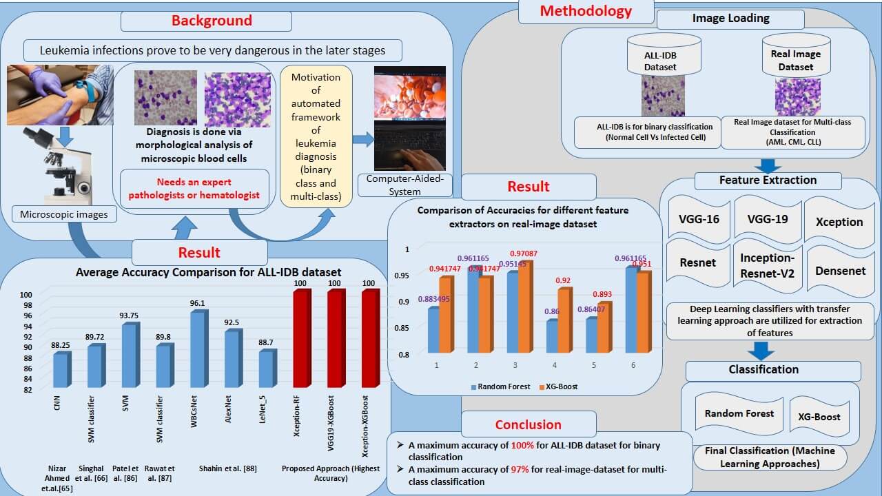
Infection of leukemia in humans causes many complications in its later stages. It impairs bone marrow’s ability to produce blood. Morphological diagnosis of human blood cells is a well-known and well-proven technique for diagnosis in this case. The binary classification is employed to distinguish between normal and leukemia-infected cells. In addition, various subtypes of leukemia require different treatments. These sub-classes must also be detected to obtain an accurate diagnosis of the type of leukemia. This entails using multi-class classification to determine the leukemia subtype. This is usually done using a microscopic examination of these blood cells. Due to the requirement of a trained pathologist, the decision process is critical, which leads to the development of an automated software framework for diagnosis. Researchers utilized state-of-the-art machine learning approaches, such as Support Vector Machine (SVM), Random Forest (RF), Naïve Bayes, K-Nearest Neighbor (KNN), and others, to provide limited accuracies of classification. More advanced deep-learning methods are also utilized. Due to constrained dataset sizes, these approaches result in over-fitting, reducing their outstanding performances. This study introduces a deep learning-machine learning combined approach for leukemia diagnosis. It uses deep transfer learning frameworks to extract and classify features using state-of-the-art machine learning classifiers. The transfer learning frameworks such as VGGNet, Xception, InceptionResV2, Densenet, and ResNet are employed as feature extractors. The extracted features are given to RF and XGBoost classifiers for the binary and multi-class classification of leukemia cells. For the experimentation, a very popular ALL-IDB dataset is used, approaching a maximum accuracy of 100%. A private real images dataset with three subclasses of leukemia images, including Acute Myloid Leukemia (AML), Chronic Lymphocytic Leukemia (CLL), and Chronic Myloid Leukemia (CML), is also employed to generalize the system. This dataset achieves an impressive multi-class classification accuracy of 97.08%. The proposed approach is robust and generalized by a standardized dataset and the real image dataset with a limited sample size (520 images). Hence, this method can be explored further for leukemia diagnosis having a limited number of dataset samples.Graphic Abstract
Keywords
The ability of bone marrow to form blood results in the production of various blood components. Blood, an essential human body component, keeps the human alive. It consists of various cells such as White Blood Cells (WBC), Red Blood Cells (RBC), plasma (a fluid made up of various gases and electrolytes), and others [1]. An infection in the body alters blood components regarding their counts, size, shape, and others. These changes must be analyzed to diagnose the particular infection [2]. Leukemia is an infection that causes an increase in the number of blast cells in the blood [3]. These are immature WBC blasts. Because of the higher percentage of blasts, RBC has very little space to flow through the blood. This reduces the percentage of RBC, resulting in anemia and other abnormalities [4]. The leukemia is broadly classified as chronic and acute, with lymphoblastic and myeloid leukemia being sub-classified [5]. Fig. 1 depicts the various blood cells with and without leukemia infection.
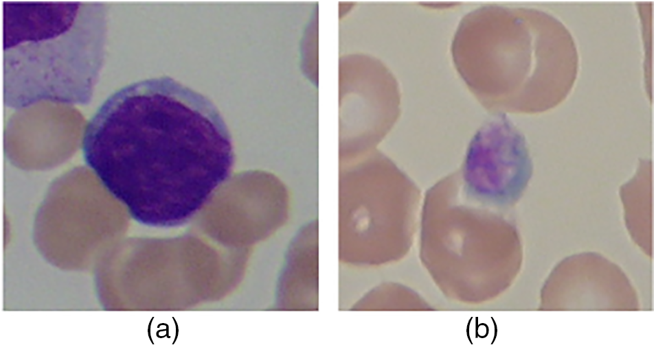
Figure 1: (a) Normal cells, and (b) Leukemia cells [6]
The best way to diagnose leukemia is to examine the morphology of white blood cells under a microscope [7]. Such diagnosis requires a highly trained and experienced pathologist [8], as the shape, size, and presence of Auer rods in the blood sample influence the decision regarding leukemia infection. This complexity in diagnostic decisions has prompted many researchers to explore the issue and develop software solutions for diagnostic purposes [9]. Various methods such as SVM [10], Näive Bayes [11], decision trees [12], random forest [13], XGBoost [14], AdaBoost [15], CNN [16], and other software algorithms are employed by researchers for diagnostic decisions.
Traditional image processing techniques like thresholding [17], edge detection [18], and contour detection [19] are employed to detect and segment leukemia. These techniques offer optimal accuracies compared to machine learning and deep learning methods [20]. However, to enhance system robustness and improve diagnostic accuracy, more advanced techniques, including machine learning and deep learning, are employed [21]. Due to the limited number of sample images in medical datasets, deep learning techniques can lead to overfitting [22], affecting detection accuracy [23]. However, there exists a trade-off between accuracy and interpretability with machine learning [24].
In order to address these challenges, this study presents a hybrid approach to harness the strengths of both machine learning and deep learning models. In many strategies, machine learning or deep learning classifiers are used exclusively. Given the limited sample images, deep learning classification can result in overfitting, thereby limiting accuracy. Thus, instead of relying solely on deep learning, the approach is hybridized with cutting-edge machine learning algorithms. Transfer learning frameworks are employed solely for feature extraction. These features are then passed to machine learning algorithms for the final classification. This approach is innovative and robust for limited dataset images, achieving an accuracy of 100% for the standard dataset (ALL-IDB) and approaching 96% for multi-class classification of the real-image-dataset.
The paper’s second section introduces the proposed methodology and dataset, followed by the results and discussion section. The conclusion is then presented, accompanied by remarks on future work directions.
There are different traditional image processing and machine learning approaches employed by researchers for leukemia detection, such as support vector machine (SVM) [25–28], SVM and k-means clustering [29], K-nearest neighbor (KNN) and Naïve Bayes [30], KNN [31], Zack algorithm [32,33], and deep learning approaches such as CNN [34], deep learning nets [35], CNN plus SVM approach [36,37], AlexNet [38,39], Ensembles of CNN [40], a special CNN called ConVNet [41], and ANN [42]. Singhal et al. [43] used a support vector machine (SVM) classifier for leukemia detection. This work utilized features including geometry and local binary pattern (LBP), which achieved accuracies of 88.79% and 89.72%, respectively.
Mohamed et al. [44] presented a study on the diagnosis of sub-classes of leukemia, viz. (ALL and AML) and Myeloma. Features were extracted via methods such as scale-invariant feature transform (SIFT), speeded-up robust features (SURF), and oriented FAST and rotated BRIEF (ORB) approaches. These different features were combined and passed to classifiers, such as SVM, K-nearest neighbor (KNN), and random forest (RF). The accuracy of their approach reached 94.3% using the RF classifier. Here, pre-processing and segmentation stages should be included for better results. After this, different features such as area, perimeter, statistical feature, and gray-level-co-occurrence-matrix are utilized, and these were hand-crafted. Instead of using hand-crafted features, more sophisticated deep learning feature extractors could improve performance. Also, DL feature extractors could be tested for better results without segmentation.
Mohapatra et al. [45] used an ensemble classifier in which the data were segmented before classification. Afterward, feature extraction was performed considering different morphological and textural features. Their results were compared with state-of-the-art machine learning algorithms (Naïve Bayes, KNN, multilayer perceptron, SVM, radial basis functional network) and were found superior with an accuracy of 94.73%. This work produces sub-images consisting of a single malignant-infected cell. Hence, during the analysis of real images, this work might fail to demonstrate its robustness and generalization. Additionally, this work experiments on binary classification, but in a practical scenario, there is a need to classify different sub-classes of leukemia, necessitating multi-class classification.
Mishra et al. [46] proposed a feature extractor based on the gray-level co-occurrence matrix (GLCM). Probabilistic principal component analysis was also used, followed by an RF classifier. This method used marker-based segmentation before the application of RF, which can be removed when DL methods are applied. This method deals only with binary classification, considering ALL and normal cells. Multi-class classification with leukemia sub-classes is not addressed in this work. Das et al. [47] employed feature extraction based on the gray-level-run-length matrix (GLRLM) and GLCM texture features, and they also considered color and shape features. The most prominent features were selected based on PCA and then used with an SVM for binary leukemia classification. This method segments sub-images based on which leukemia decisions are made. When a larger dataset is used, this sub-image segmentation takes longer, increasing the time required for classifier decisions. Real image datasets contain many leukocyte blasts, making it challenging to segment each via sub-image segmentation. The number of blasts determines the disease’s severity. Hence, applying this method to a real-image dataset may challenge the achievement of good accuracies.
Abdeldaim et al. [48] proposed a system that extracted different features, including shape, color, texture, and hybrid features. After normalizing these features, several state-of-the-art machine learning algorithms were used for final classification, such as Naïve Bayes with Gaussian distribution, decision tree, SVM with RBF kernel, and KNN. In their work, only binary classification is considered, and sub-classes of leukemia are not addressed. In research, Mandal et al. [49] used a decision tree (DT) with Gradient Boosting for the classification of Acute Lymphoblastic Leukemia (ALL). This work did not measure the accuracy metric; instead, the F1-score was considered with sensitivity and specificity. The maximum F1-score was 85%, which could be improved further. Mishra et al. [50] conducted experimentation using a discrete orthogonal S-transform and linear discriminant analysis (LDA) feature extractors. The final classification was done with the AdaBoost algorithm. This work addresses only the binary classification of leukemia, detecting normal and infected cells. Different leukemia subtypes also need to be predicted in a practical scenario, and multi-class classification must be implemented. Al-Jaboriy et al. [51] used artificial neural networks (ANN) with a four-moment statistical feature extraction stage. The accuracy obtained in this technique was 97%, but the algorithm should be generalized by applying it to a real-image dataset and considering multi-class classification to identify the sub-classes of leukemia.
In 2020, Banik et al. [52] applied a convolutional neural network (CNN)-based approach for detecting white blood cells in microscopic blood images. In this method, the features from the first and last layers were combined to enhance performance. Pre-processing and segmentation were conducted before extracting features via the CNN. This approach should be generalized by considering a real-image dataset. Honnalgere et al. [53] used the VGG16 framework with transfer learning from a pre-trained model on the ImageNet dataset. Batch normalization and data augmentation helped achieve a larger sample size. Their experiments resulted in a precision, recall, and F1-score of 91.70%, 91.75%, and 91.70%, respectively. Shah et al. [54] introduced a method that combined CNN and a recurrent neural network (RNN), achieving an accuracy of 86.6%. Although decent, this can be improved. Yu et al. [55] explored this area with a CNN-based approach, considering and combining different frameworks such as ResNet50 [56], InceptionV3 [57], VGG16 [58], VGG19 [59], and Xception. Their methods achieved an accuracy of 88.5%. Pan et al. [60] proposed an approach using a pre-trained RNN with various feature extraction and combination stages, claiming an F1-score of 92.50%. Marzahl et al. [61] employed the ResNet18 deep learning framework to detect leukemia and normal cells. With advanced dataset augmentation, they achieved an F1 score of 87.46%. Still, there is a need for more reliable and robust methods, especially for smaller datasets. The methods by [54–60] achieved accuracy up to 92.50%, and the same researchers [54–60] tested binary classification on the standard ALL-IDB datasets. Hence, it is necessary to generalize and fortify these methods by applying them to a real-image dataset with multi-class classification.
In a separate work, Mittal et al. [62] presented a review of leukemia detection using blood smear images. They explored blood components, databases, leukemia types, and various methodologies for leukemia detection. Different steps, such as pre-processing, segmentation, feature extraction, and classification methods employed by various researchers, are reviewed in this study. The challenges faced by classifiers, including large training data, achieving good accuracy, generalization, and reproducibility, are highlighted in this survey. The need for data augmentation is also discussed.
The need for a large dataset and augmentation, as mentioned by Mittal et al. [62], can be addressed by employing a hybrid approach that combines deep learning and machine learning. The number of required dataset images can be reduced if deep learning is used for feature extraction and machine learning for the final classification.
Although the methods discussed in the previous section achieved reasonable accuracies, there is still room for improvement. While deep learning algorithms offer higher accuracies compared to traditional algorithms [63], the challenge lies in the dataset’s image size. For leukemia, there is a limitation on the number of images in the dataset. Consequently, deep learning algorithms might face over-fitting during training. Thus, this study introduces a solution using a hybrid machine learning-deep learning (ML-DL) combination. Features are extracted through a deep learning framework, and classification is executed using RF and XGBoost algorithms. This experiment achieved notable results using the publicly available dataset (ALL-IDB) and a private real-image dataset.
The ALL-IDB1 dataset contains 109 images, while the ALL-IDB2 has 260. For multi-class classification, there are 528 images divided into three sub-classes. Since deep learning is employed solely for automatic feature extraction and not for classification, there is no risk of overfitting during experimentation. Although data augmentation is typically employed to increase sample sizes, achieving the desired accuracy with the available samples meant that augmentation was unnecessary in this study. The proposed approach, combining deep learning and machine learning, promises enhanced performance for datasets with limited images, applicable to binary and multi-class classification.
Fig. 2 shows the proposed hybrid approach methodology for the diagnosis of leukemia via binary classification and multi-class classification.
Figure 2: Proposed methodology of leukemia classification
Images from the dataset are loaded to process them and propagate in further stages for classification. ALL-IDB dataset is used for the processing.
There are different frameworks available with convolutional neural networks. Some popular frameworks, including VGG16, VGG19, ResNet50, Xception, Inception-ResNet-v2, and Densenet, are employed for feature extraction. These architectures are explained below.
3.2.1 VGGNet [64]
CNNs’ depth was increased with VGG to improve model performance. Visual Geometry Group, or VGG, is a typical deep CNN architecture with several layers. Two classical models were developed as VGG, namely VGG16 and VGG19. Fig. 3 depicts a typical VGG16 architecture. Very tiny convolutional filters are used in the construction of the VGG network. A total of sixteen layers, of which three are fully connected, and thirteen convolutional layers are present in the VGG16 network. The VGGNet accepts input of size 224 × 224-sized images.
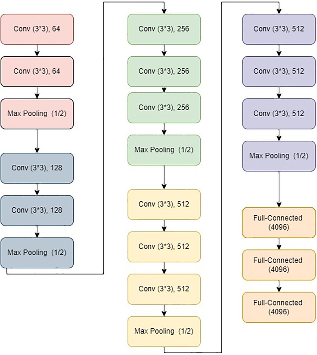
Figure 3: VGG16 architecture
Convolutional layers: This layer uses a receptive field of 3 × 3 to record two movements, viz. left to right and up to down. Additionally, 1 × 1 convolution filters are employed for the linear transformation of the input. The next part is a ReLU unit, a progressive step over AlexNet regarding training time [65]. The convolution stride is set to 1 pixel to maintain spatial resolution. The stride represents the number of pixel shifts across the input matrix.
Hidden layers: These layers primarily make use of ReLU. Local Response Normalization (LRN) is commonly avoided when using VGG because it increases memory usage and training time. Furthermore, it does not affect overall accuracy.
Fully-connected layers: It has three layers that are fully connected. The first two levels have 4096 channels each. The third layer has 1000 channels, one for each class.
3.2.2 ResNet [66]
ResNet50, as shown in Fig. 4, is a variant of a typical Reset model. It has 50 layers in total. The model consists of 48 convolutional, one maximum pool, and one average pooling layer. It has one convolution layer having a 7 × 7 kernel size and distinct kernels of 64. All layers have a stride size of 2. After this, there is a max pooling layer with a size of stride 2. Another convolution contains a 1 × 1 layer, with 64 kernel, then a 3 × 3 sized kernel, which continues with a 64 kernel and a 1 × 1, 256 kernel. This phase has nine layers. Following that, there is a kernel of 1 × 1, 128. After this, 3 × 3, 128 kernel and a kernel of 1 × 1, 512 size at the final stage.
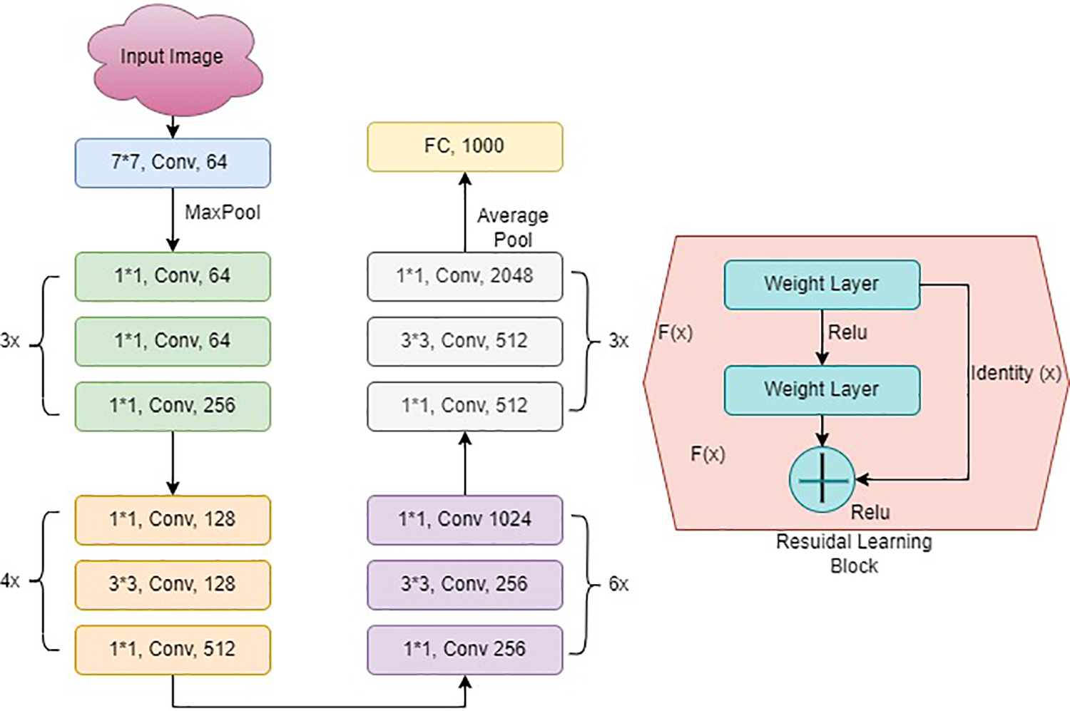
Figure 4: ResNet architecture
This stage was repeated four times, which resulted in 12 layers. After this stage, there are different combinations, including 1 × 1, 3 × 3, and 1 × 1, with convolution filter sizes of 256, 256, and 512, respectively, repeated six times. The sequence of 1 × 1, 3 × 3, and 1 × 1 was repeated with convolution filter sizes of 512, 512, and 2048, respectively. A fully connected layer of 1000 nodes comes at the last with the Softmax function.
3.2.3 XceptionNet [67]
This has depth-wise separable convolutions. Xception is another name for an “extreme” version of an Inception module. Xception is an abbreviation for “extreme inception”, it uses the Inception principles. There is a use of 1 × 1 convolutions to compress the original input in Inception, and different filters were used on each depth space from each input space. Xception simply reverses this step. This method is nearly identical to the depth-wise separable convolution used in designing the neural network. There is one more distinction between Inception and Xception. The presence or absence of a nonlinearity following the initial operation. A ReLU nonlinearity follows both operations in the Inception model, whereas Xception does not. The data is processed after passing through the entry flow, through the middle flow (which repeats eight times), and through the exit flow. Fig. 5 shows the detailed architecture of XceptionNet.
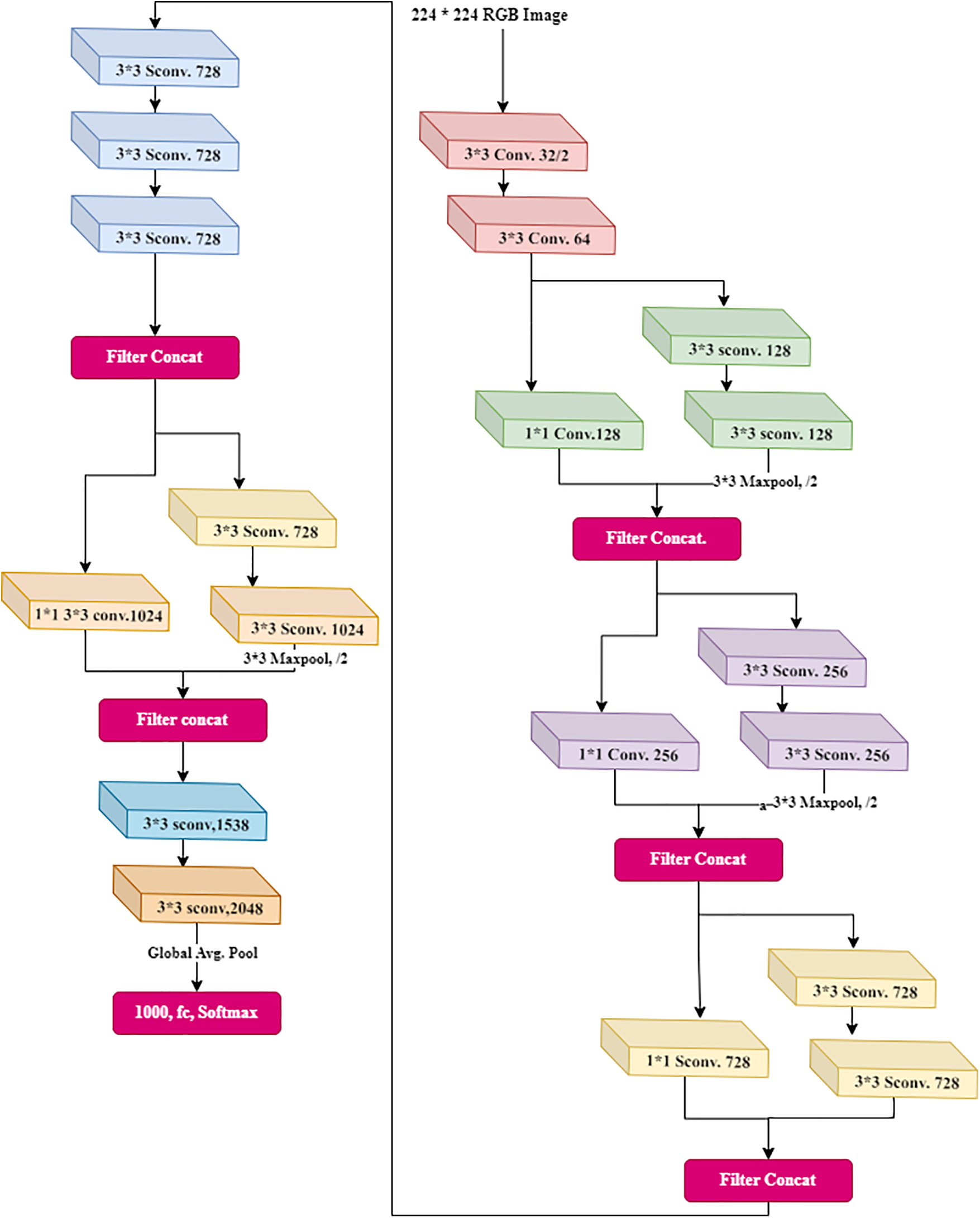
Figure 5: Xception architecture
3.2.4 Inception-ResNet-v2 [68]
Inception-ResNet-v2 was trained with a vast number of images from the ImageNet database. The 164-layer network can classify images into numerous additional object categories, allowing it to learn detailed representations of features for a wide range of images. The input to the network is a 299 × 299 image, and it produces class probabilities at the output. This network is a combination of Inception and residual connections [69]. It has a residual connection with a combination of convolutional filters of multiple sizes. Due to the use of the residual connections, the degradation issue was compensated, and training time was also reduced to some extent. Fig. 6 shows the basic network architecture of Inception-ResNet-v2.

Figure 6: Inception-ResNet-Version-2 architecture
3.2.5 Densenet [70]
Fig. 7 shows a Densenet architecture consisting of low level layers, high level layers, upsampling layers, and integration layers. Densenet has shorter connections between the layers, making it efficient during training [71]. Each layer is deeply connected to the other, ensuring the free flow of information within the network. Every layer receives input from previous layers to maintain the feed-forward nature. This input is then passed on to subsequent layers via its feature maps. There is the concatenation of features of different layers. So, the ith layer has I input and comprises feature maps from all previous convolutional blocks. All subsequent ‘I-i’ layers receive their feature maps. In contrast to traditional deep learning architectures, this introduces ‘(I(I + 1))/2’ connections into the network. It requires fewer parameters than traditional CNN because it does not need to learn unimportant feature maps. Densenet has two crucial blocks besides the basic convolutional and pooling layers. They are known as Transition Layers and Dense Blocks.
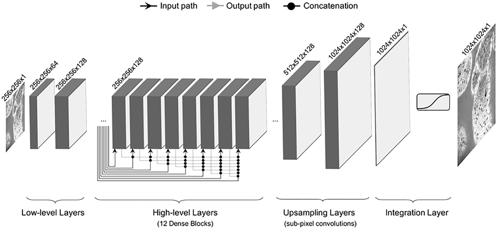
Figure 7: Densenet architecture
After the feature extraction, popular state-of-the-art, classical machine learning algorithms are employed for classification. RF and XGBoost classifiers are utilized after the feature extraction via deep learning frameworks.
For this stage, RF and XGBoost classification techniques are employed.
These models predict output by combining the outcomes of multiple regression decision trees [72]. The architecture of RF is shown in Fig. 8. It has many decision trees, each with its training dataset. As a result, this algorithm performs better in classification problems than a decision tree [73]. The pruning method selection and the branching criteria are regarded as the two most important factors [74]. This algorithm is determined by the number of created trees and the utilized samples by a particular node. Each tree is generated independently as a random vector sampled from input data, while the forest’s tree distribution remaining constant. The forest predictions are averaged using bootstrap aggregation and random feature selection [75].

Figure 8: RF architecture
Extreme Gradient Boosting (XGBoost) is a scalable, distributed gradient-boosted decision tree (GBDT) machine learning library [76]. It works with many problems, including classification, regression, and ranking. This algorithm supports parallel tree boosting [77]. Gradient-boosted decision trees are implemented in XGBoost, which are dominant in many cases [78]. This algorithm sequentially generates decision trees [79]. Weights are crucial in XGBoost [80]. The architecture of XGBoost is shown in Fig. 9. In this algorithm, the weights are assigned to each independent variable. These weights are then transferred into the decision tree, which predicts the outcome. The weight of variables incorrectly predicted by the tree is increased, and these variables are input into the second decision tree. Then, individual classifiers and predictors are combined to create a more robust and precise model. It can solve regression, classification, ranking, and user-defined prediction problems [81].

Figure 9: XGBoost architecture
3.3.3 Hyperparameter Tuning of Model
As explored in Subsection 3.3.2, two state-of-the-art machine learning models are employed for final classification, including RF and XGBoost. The following steps were used for the tuning of hyperparameter of the classification models:
1. RF is tuned with n_estimators (no. of trees). It has experimented with the number of trees with values of 1 to 100.
2. For getting the best value of n_estimaters, the GridSearchCV object is used. It performs an exhaustive search over the hyperparameter grid, fitting and evaluating the RF model for the specified values of trees.
3. Cross-validation is employed to estimate the model’s performance, and the value of n_estimater obtained is 24. Hence, fine-tuning is done to get the value of 24 trees.
4. XGBoost is tuned for n_estimators, maximum depth, and Gamma. These parameters are tuned by considering n_estimators, Maximum depth, and Gamma.
5. With the GridSearchCV object, the parameters are obtained after the tuning with the following values. In order to find the best values of these parameters, these parameters are tested with values as n_estimators with 10, 20, 40, and 100; max_depth: 3, 4, and 5; Gamma with the values as 0, 0.15, 0.30, 0.50, and 1.
6. Finally, the values of these parameters obtained for the best accuracies with cross-validation of 5 for the XGBoost are as follows:
i) N_estimators = 10
ii) Maximum Depth = 3
iii) Gamma = 0
Classification of normal and abnormal cell images and multi-class classification are the prime motivations of the presented work. Different metrics are employed to evaluate the performance of the proposed system. Following are the parameters utilized for accuracy measurement:
Accuracy [82]:
where TP = true positive, TN = true negative, FP = false positive, FN = false negative.
Recall [83]:
Precision [84]:
F1-score [85]:
Confusion matrix [86]:
A confusion matrix is often employed to demonstrate classifier performance based on the four values listed above (TP, FP, TN, and FN). When these are plotted against each other, a confusion matrix is formed.
This study utilizes A very popular dataset employed by many researchers, i.e., ALL-IDB1 and ALL-IDB2. Figs. 10a and 10b show images from the ALL-IDB1 dataset, while Figs. 10c and 10d show images from the ALL-IDB2 dataset. This database is used for acute leukemia analysis and research. This dataset has two subtypes: ALL-IDB1 and ALL-IDB2. All images were captured using a Canon Powershot G5 camera. The microscope’s magnification range was between 300 and 500. JPEG images with a 24-bit color depth were used. The ALL-IDB1 dataset contains 109 images with a total element count of 3,900 and a resolution of 2592 * 1944. There are 510 lymphoblasts in total. The ALL-IDB2 dataset consists of 260 images with a total element count of 257 and a resolution of 257 × 257. It has a total of 130 lymphoblasts.
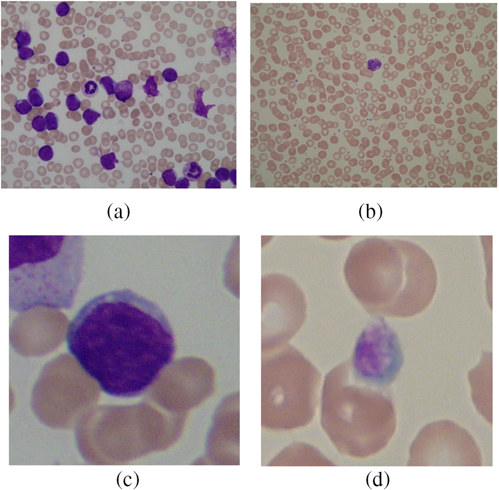
Figure 10: (a) ALL-IDB1 infected image; (b) ALL-IDB1 normal image; (c) ALL-IDB2 infected image; (d) ALL-IDB2 normal image
4.2 Private Real Images Dataset
In addition to this dataset, a real image dataset is also utilized for the experiment. The dataset is a multi-class dataset with three sub-classes of leukemia, namely acute myeloid leukemia (AML), (Chronic myeloid leukemia) CML, and (Chronic lymphocytic leukemia) CLL. The AML class contains 181 images, while the CLL and CML have 166 and 173 images, respectively. Figs. 11a–11c show images from the dataset with CLL, CML, and AML types, respectively. This dataset contains 520 images of blood slides from three classes. This dataset was provided by Nidan Diagnostic in Ahmednagar, India.
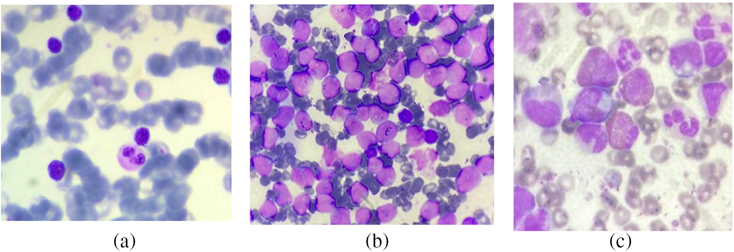
Figure 11: Images from the real dataset: (a) CLL; (b) CML; (c) AML
The experimentation was conducted in two ways. A binary classification was performed on ALL-IDB1 and ALL-IDB2 datasets, which output metrics showing the normal cell and infected cells’ classification. Subsequently, a real-image dataset consisting of different sub-classes of leukemia (AML, CML, and CLL) was tested, yielding a multi-class classification. The following sections discuss this in detail.
Performance metrics considering ALL-IDB1 and ALL-IDB2 datasets for binary classification of leukemia cells and normal cells are shown in this section.
Figs. 12a–12d show the confusion matrix as an outcome of VGG16 as a feature extractor and RF, and XGBoost classifier for ALL-IDB1 and 2 datasets.
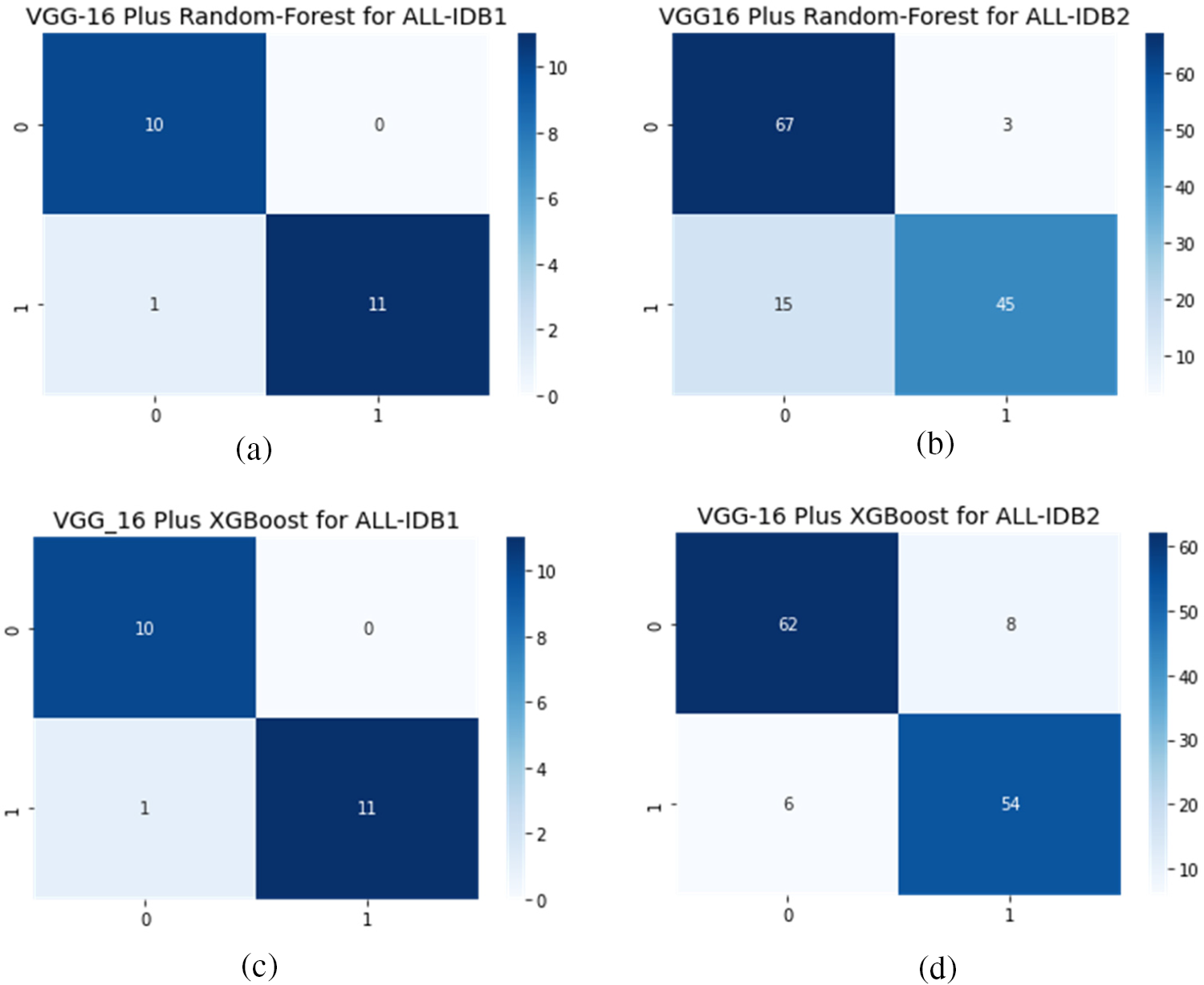
Figure 12: Confusion matrix considering VGG16 as feature extractor: (a) VGG16 plus RF for ALL-IDB1 dataset; (b) VGG16 plus RF for ALL-IDB2 dataset; (c) VGG16 plus XGBoost for ALL-IDB1 dataset; (d) VGG16 plus RF for ALL-IDB2 dataset
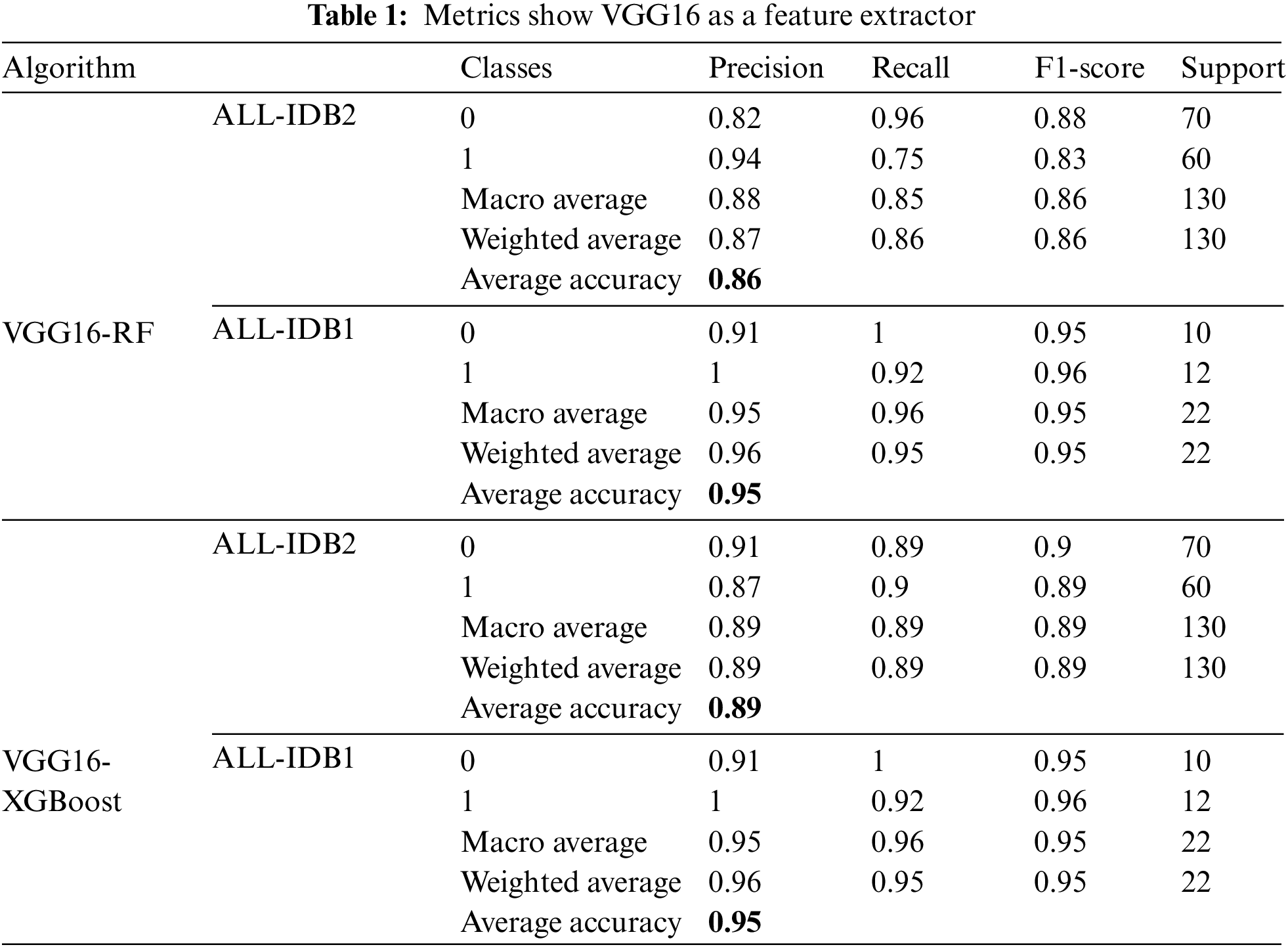
Table 1 shows performance measures using VGG16 as the feature extractor and two classical machine learning algorithms for final classification. RF and XGBoost are employed for classification. Different measures are presented, including precision, recall, F1-score, and accuracy. ALL-IDB1 and ALL-IDB2 both are applied for the analysis. Precision varies from 0.87 to 0.96 for both parts of the dataset. Recall takes the value from 0.86 to 0.96, while the F1-score varies from 0.86 to 0.95 in the case of RF and XGBoost with ALL-IDB1 and ALL-IDB2. The accuracy reaches a peak of 95.45% for the ALL-IDB1 dataset.
Figs. 13a–13d show the confusion matrices as outcomes of VGG19 used as a feature extractor, combined with RF and XGBoost classifiers, for the ALL-IDB1 and 2 datasets.

Figure 13: Confusion matrix considering VGG19 as feature extractor: (a) VGG19 plus RF for ALL-IDB1 dataset; (b) VGG19 plus RF for ALL-IDB2 dataset; (c) VGG19 plus XGBoost for ALL-IDB1 dataset; (d) VGG19 plus RF for ALL-IDB2 dataset
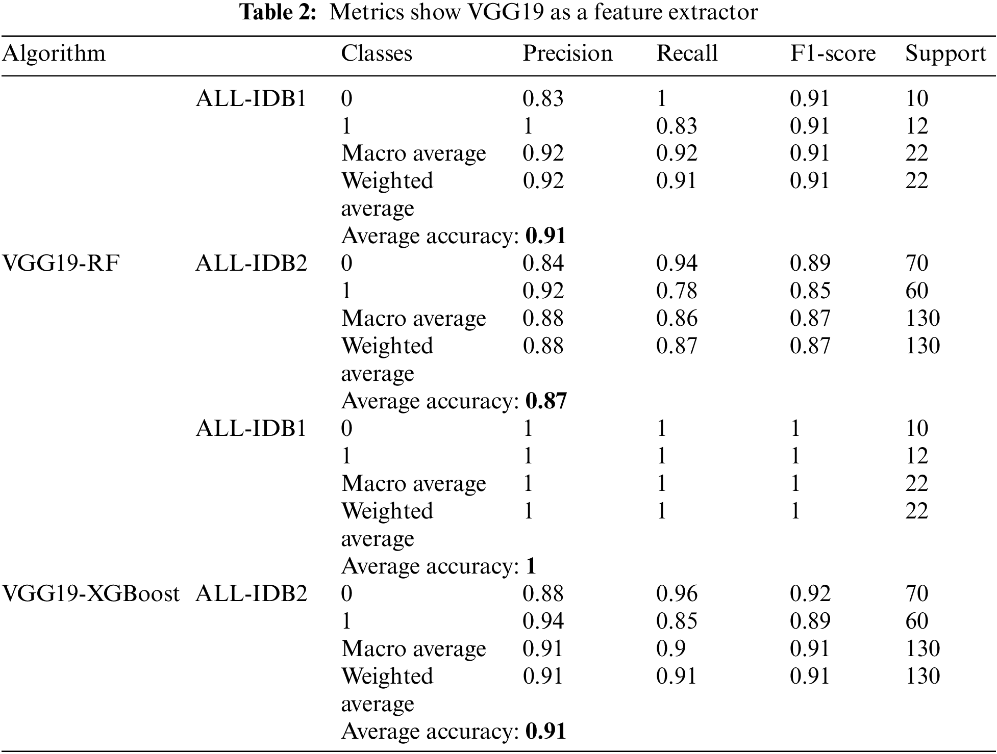
As indicated in Table 2, VGG19 is used as a feature extractor, and RF and XGBoost are employed for final classification. The precision obtained in this case is 0.88 to 0.92, which is a good and permissible value. Recall also varies from 0.87 to 0.91, and the score range is from 0.87 to 0.91. The maximum accuracy value is over 90% for both datasets and the machine learning classifiers.
5.1.3 Xception as a Feature Extractor
Figs. 14a–14d show the confusion matrix as an outcome of Xception as a feature extractor and RF and XGBoost classifiers for ALL-IDB1 and two datasets.

Figure 14: Confusion matrix considering Xception as feature extractor: (a) Xception plus RF for ALL-IDB1 dataset; (b) Xception plus RF for ALL-IDB2 dataset; (c) Xception plus XGBoost for ALL-IDB1 dataset; (d) Xception plus RF for ALL-IDB2 dataset
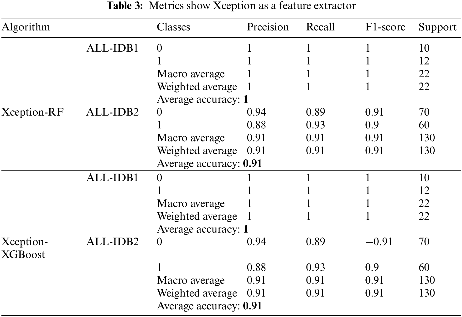
Table 3 shows the results obtained utilizing Xceptionnet as a feature extractor, with RF and XGBoost as the final classifiers. Parameters, such as precision, recall, and F1-score, vary from 0.90 to 1. As far as accuracy is concerned, it ranges from 90% to 100% in the cases mentioned above.
5.1.4 ResNet Feature Extractor
Figs. 15a–15d show the confusion matrices as outcomes of ResNet50 used as a feature extractor, in combination with RF and XGBoost classifiers, for the ALL-IDB1 and ALL-IDB2 datasets.

Figure 15: Confusion matrix considering ResNet as feature extractor: (a) ResNet plus RF for ALL-IDB1 dataset; (b) ResNet plus RF for ALL-IDB2 dataset; (c) ResNet plus XGBoost for ALL-IDB1 dataset; (d) ResNet plus RF for ALL-IDB2 dataset
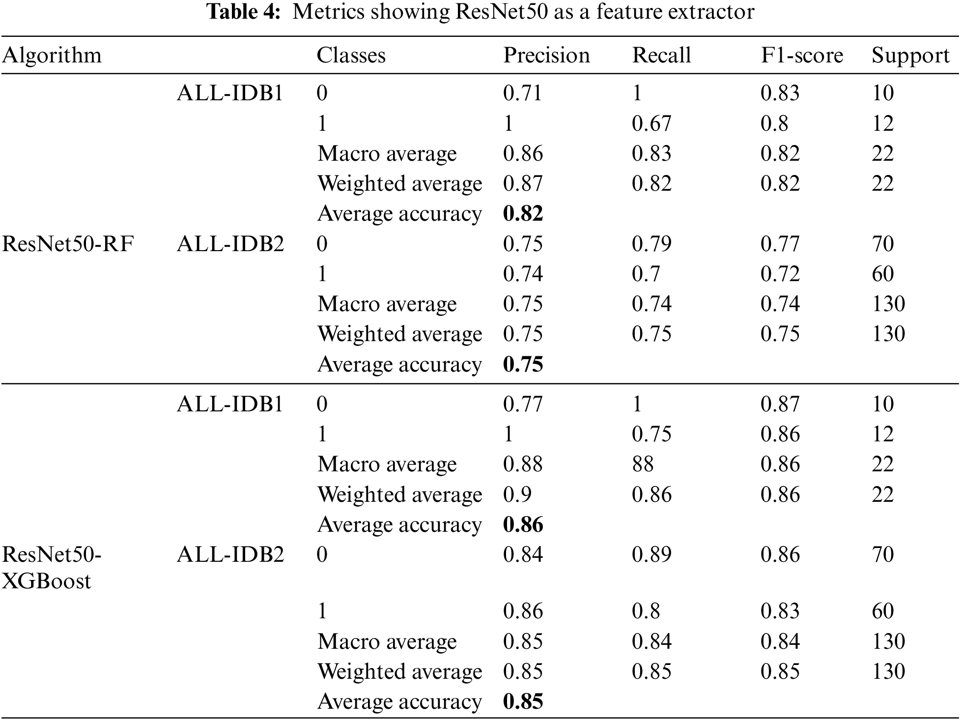
ResNet50 is used as a feature extractor using a transfer learning approach in the next case. After extracting features, they are passed through RF and XGBoost algorithms. Different metrics obtained with these approaches are listed in Table 4. Precision, recall, and F1-score achieve a maximum value of 0.86, while the maximum accuracy is 86%.
5.1.5 InceptionResNetV2 Feature Extractor
Figs. 16a–16d show the confusion matrices as outcomes of InceptionResNetV2 used as a feature extractor, in combination with RF and XGBoost classifiers, for the ALL-IDB1 and ALL-IDB2 datasets.
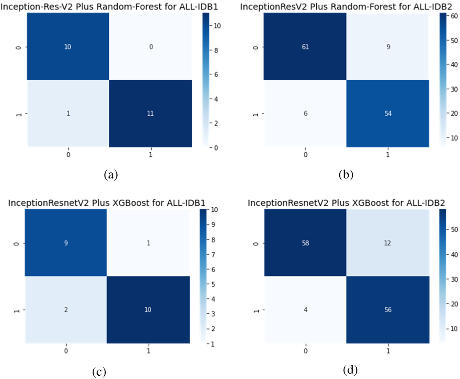
Figure 16: Confusion matrix considering Inception-ResNet-V2 as feature extractor: (a) Inception-ResNet-V2 plus RF for ALL-IDB1 dataset; (b) Inception-ResNet-V2 plus RF for ALL-IDB2 dataset; (c) Inception-ResNet-V2 plus XGBoost for ALL-IDB1 dataset; and (d) Inception-ResNet-V2 plus RF for ALL-IDB2 dataset
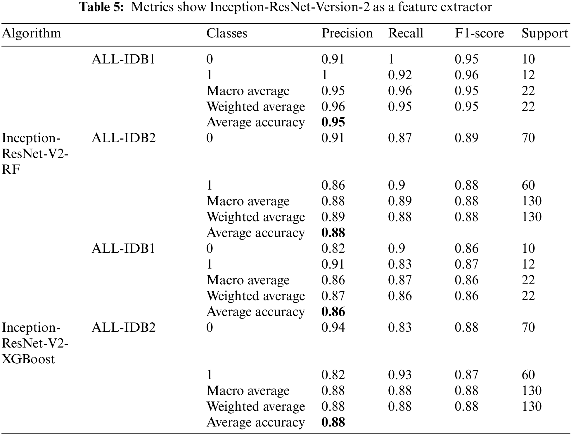
There is a popular framework consisting of Inception-Restnet-Version-2, which is used as a feature extractor, and both RF and XGBoost as the final stage of the classifier. Table 5 shows the different performance measures in this case. It indicates that precision, recall, and F1-score approaches a maximum of 0.96 and a minimum of 0.86. The maximum and minimum accuracy values are 95% and 86%, respectively. In addition to these networks, Denset is employed to extract features, which are passed through RF and XGBoost algorithms for the final classification. As shown in Table 6, Inception-ResNet-V2 is utilized as a feature extractor, producing a maximum precision of 94%, a maximum recall value obtained of 96%, and the F1-score achieves a maximum value of 95%. For this approach, accuracy ranges from 88% to 95%.
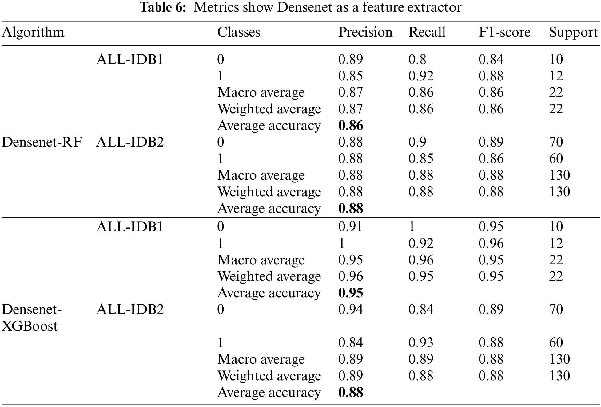
5.1.6 Densenet Feature Extractor
Figs. 17a–17d show the confusion matrices as outcomes of Densenet used as a feature extractor, in combination with RF and XGBoost classifiers, for ALL-IDB1 and ALL-IDB2 datasets.

Figure 17: Confusion matrix considering Densenet as feature extractor: (a) Densenet plus RF for ALL-IDB1 dataset; (b) Densenet plus RF for ALL-IDB2 dataset; (c) Densenet plus XGBoost for ALL-IDB1 dataset; (d) Densenet plus RF for ALL-IDB2 dataset
Fig. 18 shows the graphical representation of accuracies obtained by different approaches for binary classification of leukemia, considering datasets ALL-IDB1 and ALL-IDB2. It indicates that the accuracies of the XGBoost classifier with different feature extractor is greater than RF in most cases, except Densenet and Inception-ResNet-V2 as feature extractors. It approaches 100% in Xception and VGG19 as feature extractors.

Figure 18: Comparison of average accuracies of different approaches for: (a) ALL-IDB1; (b) ALL-IDB2 dataset
5.2 Multi-Class Classification
Performance metrics consider real image datasets for leukemia sub-classes multi-class classification with Acute Myloid Leukemia (AML), Chronic Myloid Leukemia (CML), and Chronic Lymphocytic Leukemia (CLL) types. Figs. 19a–19f show the confusion matrices as outcomes of different feature extractors with RF classifiers for the ALL-IDB1 and ALL-IDB2 datasets.

Figure 19: Confusion matrix of different feature extractors with RF classifier for real image dataset: (a) VGG16 plus RF; (b) VGG19 plus RF; (c) Xception plus RF; (d) ResNet50 plus RF; (e) Inception-ResNet-V2 plus RF; (f) Densenet plus RF
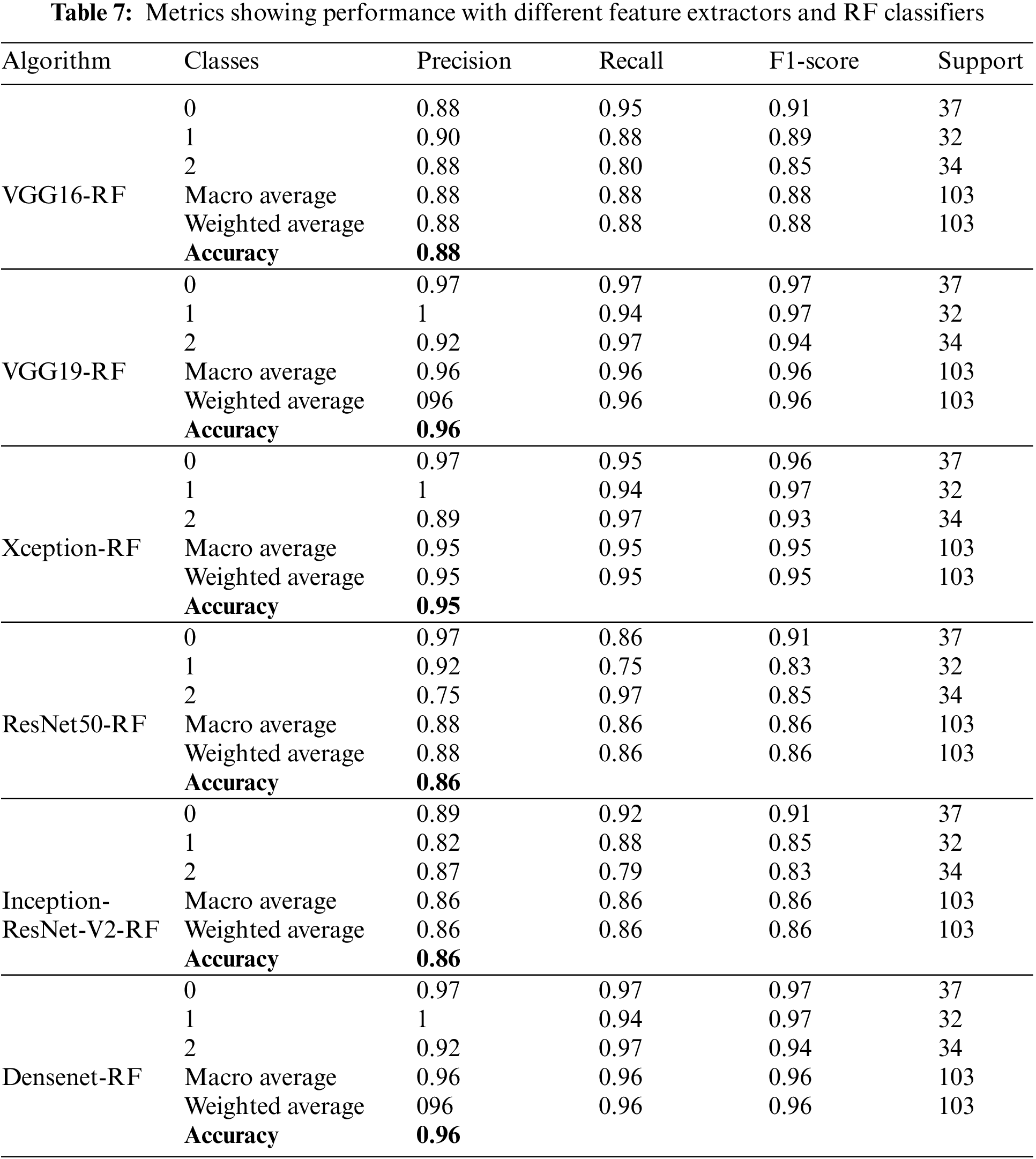
Table 7 shows different performance metrics with RF for real-image multi-class datasets. All these results are obtained utilizing the real image dataset. Precision value achieves a maximum value of 96% for Densenet and VGG16 feature extractors, while recall achieves a maximum value of 96% for Densenet F1-score, which also achieves a 9% maximum value for Densenet. A good and acceptable range is obtained as the accuracies are observed in this part of the experimentation. It ranges from 88% to 96%.
Figs. 20a–20f show the confusion matrices as outcomes of different feature extractors with XGBoost classifiers for the ALL-IDB1 and ALL-IDB2 datasets.

Figure 20: Confusion matrix of different feature extractors with XGBoost classifier for real image dataset: (a) VGG16 plus XGBoost; (b) VGG19 plus XGBoost; (c) Xception plus XGBoost; (d) ResNet50 plus XGBoost; (e) Inception-ResNet-V2 plus XGBoost; (f) Densenet plus XGBoost
Table 8 presents the performance metrics for XGBoost classification and different deep learning frameworks, including VGG16, VGG19, Xception, Inception-ResNet-V2, ResNet50, and Densenet. Precision takes the minimum value of 94% and a maximum of 95% by observing all the feature extractors’ weighted and macro average values. Recall has a maximum value of 89% and a minimum of 97%. Weighted and macro average values of the F1-score range from 89% to 97% while moving through all the feature extractors. A maximum accuracy of 97.08% is obtained with this part of the experimentation.
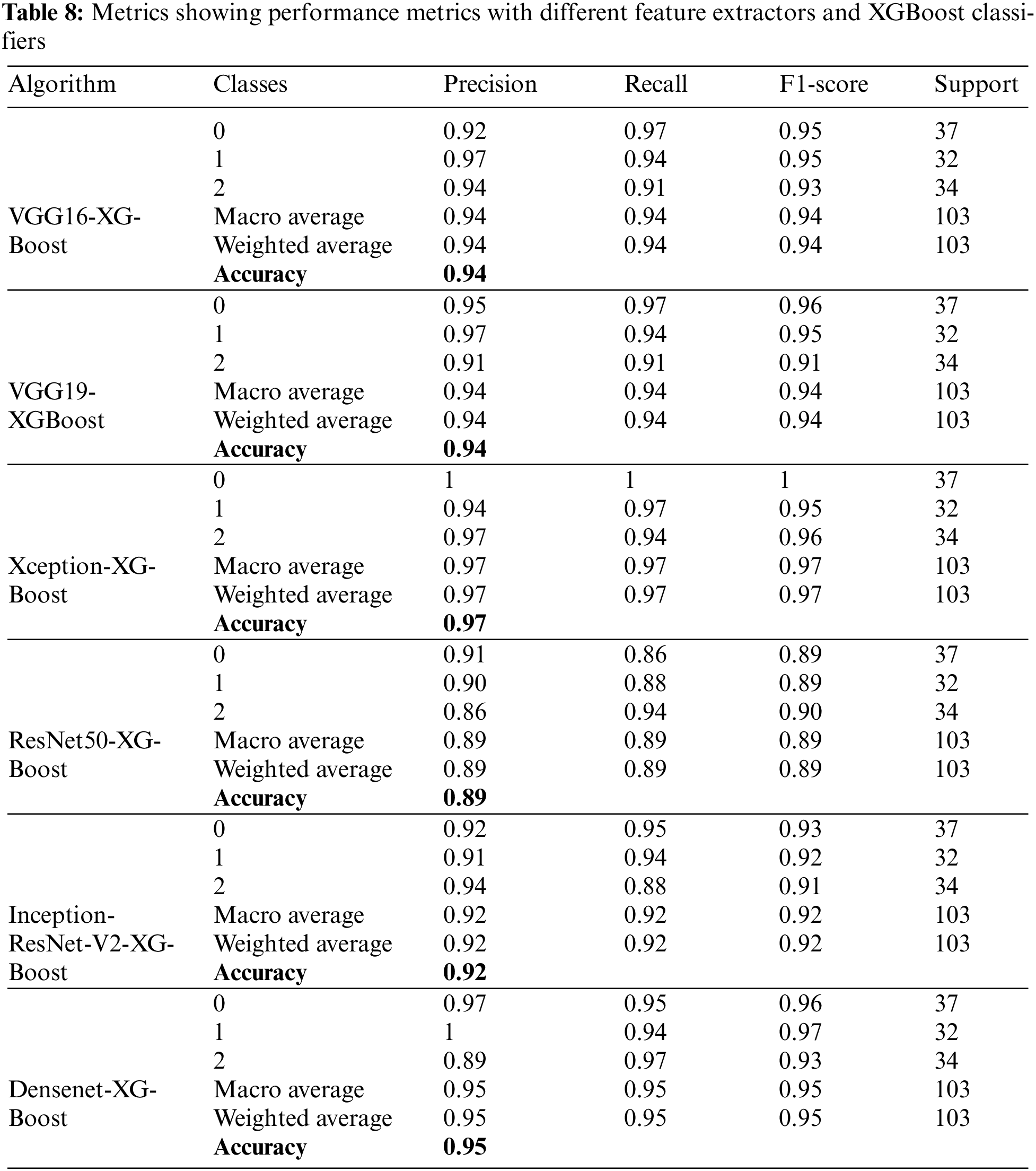
Fig. 21 compares the accuracies of various feature extractors with RF and XGBoost classifiers. In this Figs. 1–6 represent different feature extractors: VGG16, VGG19, Xception, ResNet50, InceprionResNetV2, and Densenet, respectively. The Xception and XGBoost combination achieved the maximum accuracy.

Figure 21: Accuracy comparison of different feature extractors for real image datasets
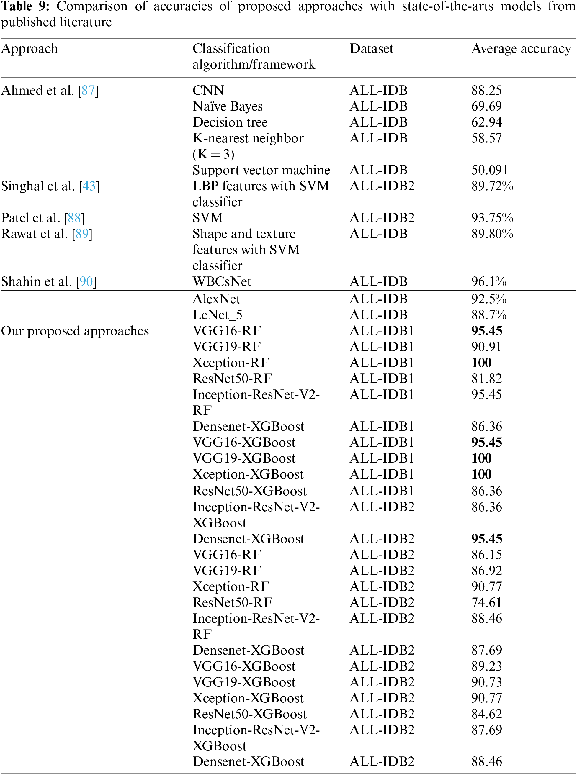
Table 9 compares the accuracy obtained by the proposed approaches with Ahmed et al. [87]. The study employed CNN classifier and other classical machine learning classifiers, including SVM, Naïve Bayes, decision trees, and KNN. With the same dataset, the accuracies in these approaches varied from 50% to 88%, with the highest accuracy for the CNN classifier. The accuracies obtained by Singhal et al. [43], Patel et al. [88], Rawat et al. [89], and Shahin et al. [90] are 89.72%, 93.75%, 89.80%, and 96.01%, respectively. The accuracies vary from 74% to 100% compared to the proposed approaches.
Leukemia is a disease that proves life-threatening in many cases at its later stages of infection. It has different sub-types, which differ in treatment guidelines. This variability in sub-types has motivated the work for multi-class leukemia cell classification. The designed framework classifies infected and normal cells in binary classification on a standard ALL-IDB dataset. Additionally, a real-image dataset consisting of leukemia sub-class images was tested with this framework for predicting the sub-type of leukemia, including AML, CML, and CLL.
The proposed approaches here are hybrid, consisting of a deep learning-machine learning (DL-ML) architecture. Popular deep learning frameworks are utilized for feature extraction with a transfer learning approach. Transfer learning frameworks VGG16, VGG19, Xception, Inception-ResNet-V2, Densenet, and ResNet are used for this purpose. If these frameworks are used for training, they may lead to over-fitting due to the limited number of dataset images. Additionally, deep learning training consumes more time as the number of epochs increases. This challenge is addressed by using these frameworks solely for feature extraction. After feature extraction, the final classification is performed by state-of-the-art machine learning models. RF and XGBoost are applied for the final classification, and various performance metrics, including precision, recall, F1-score, and accuracy, are considered for model evaluation.
Precision is a crucial metric for measuring classification results. It represents the true positive predictions against all positive predictions from the model’s testing. Various DL frameworks are combined with RF and XGBoost classifiers. Precision values obtained for VGG16, VGG19, Xception, Inception-ResNet-V2, Densenet, and ResNet feature extractors hybridized with RF for the ALL-IDB1 dataset are 0.96, 0.92, 1, 0.95, 0.87, and 0.87, respectively. For the ALL-IDB2 dataset, precision values are 0.88, 0.88, 0.91, 0.88, 0.74, and 0.88 for the above respective feature extractors. With the XGBoost classifier, the feature extractor frameworks VGG16, VGG19, Xception, Inception-ResNet-V2, Densenet, and ResNet achieved precision values of 0.95, 1, 1, 0.86, 0.95, and 0.88 for the ALL-IDB1 dataset. For the ALL-IDB2 dataset, precision values are 0.89, 0.91, 0.91, 0.88, 0.89, and 0.85 for the respective feature extractors. A notable observation from the comparison of precision values is that the XGBoost classifier consistently delivered higher precision than the RF in most cases.
Recall is another critical measure, indicating positive predictions of an experiment against true positives and false negatives. Ideally, recall should approach a value of 1, ensuring no false negatives during predictions. Recall values, calculated by considering various feature extractors used in this experimentation, for VGG16, VGG19, Xception, Inception-ResNet-V2, Densenet, and ResNet hybridized with RF for the ALL-IDB1 dataset are 0.95, 0.92, 1, 0.96, 0.82, and 0.86, respectively, with the RF classifier. For the ALL-IDB2 dataset, these values are 0.85, 0.87, 0.91, 0.89, 0.74, and 0.88 for the same feature extractors. With the XGBoost classifier, the same feature extractor frameworks achieved recall values of 0.96, 1, 1, 0.87, 0.96, and 0.88 for ALL-IDB1. ALL-IDB2 recall values are 0.89, 0.90, 0.91, 0.88, 0.89, and 0.84 for the respective frameworks. As previously observed in precision, the XGBoost classifier generally outperformed the RF in recall across most feature extractors.
The F1-score metric is also important when evaluating the performance of machine learning and deep learning models. As there is a trade-off between precision and recall, if one increases, the other decreases. To measure the performance of any model, the F1-score can prove to be a valuable measure alongside precision and recall. It essentially provides the harmonic mean of precision and recall. This metric considers both precision and recall, addressing false positives and false negatives. For all employed feature extractors, the F1-score is calculated. For the ALL-IDB1 dataset and the RF classifier, the feature extractors VGG16, VGG19, Xception, Inception-ResNet-V2, Densenet, and ResNet achieved F1-scores of 0.95, 0.91, 1, 0.95, 0.82, and 0.86, respectively. ALL-IDB2 was used for the same steps of experimentation, yielding F1-scores of 0.86, 0.87, 0.91, 0.88, 0.74, and 0.88 for the respective feature extractors. Additionally, the XGBoost classifier replaced RF, using the same feature extractors. The F1-scores obtained for VGG16, VGG19, Xception, Inception-ResNet-V2, Densenet, and ResNet were 0.95, 1, 1, 0.86, 0.95, and 0.86 for ALL-IDB1. When ALL-IDB2 was tested with the same feature extractors and XGBoost classification, the observed F1-scores were 0.89, 0.91, 0.91, 0.88, 0.88, and 0.84 for VGG16, VGG19, Xception, Inception-ResNet-V2, Densenet, and ResNet, respectively.
Another critical parameter for evaluating model performance is accuracy, which offers the number of correct predictions relative to the total predictions. For the ALL-IDB1 and ALL-IDB2 datasets, accuracy was calculated using various feature extractors and classifiers. The accuracy values for feature extractors VGG16, VGG19, Xception, Inception-ResNet-V2, Densenet, and ResNet with RF classifiers were 0.95, 0.909, 1, 0.88, 0.818, and 0.86 for the ALL-IDB1 dataset. For the ALL-IDB2 dataset, the accuracy values were 0.86, 0.87, 0.907, 0.9545, 0.74, and 0.876 for these feature extractors. XGBoost was another classifier employed in this study. The accuracy values for the frameworks above were 0.95, 1, 1, 0.876, 0.95, and 0.86 for the ALL-IDB1 dataset. For the ALL-IDB2 dataset, the accuracy values were 0.89, 0.907, 0.907, 0.86, 0.88, and 0.846 for VGG16, VGG19, Xception, Inception-ResNet-V2, Densenet, and ResNet, respectively. Accuracy generally improved with XGBoost over RF for most of the feature extractors.
The proposed approach aims to be generalized and robust by testing on a real-image dataset with multiple classes. AML, CLL, and CML sub-types of leukemia are diagnosed in the second step of this work. Precision, recall, F1-score, and accuracy are the metrics for performance evaluation in this phase. The values for feature extractors VGG16, VGG19, Xception, Inception-ResNet-V2, Densenet, and ResNet were 0.88, 0.96, 0.95, 0.86, 0.96, and 0.88 with the RF classifier. For the XGBoost classifier, these values were 0.94, 0.94, 0.97, 0.92, 0.95, and 0.89 for the same feature extractors. For recall, the real-image dataset yielded values of 0.88, 0.96, 0.95, 0.86, 0.96, and 0.86 with RF. Using XGBoost, the recall values were 0.94, 0.94, 0.97, 0.92, 0.95, and 0.89 for these feature extractors. The F1-score was also calculated using both RF and XGBoost classifiers. The values were 0.88, 0.96, 0.95, 0.86, 0.96, and 0.86 with RF, and 0.94, 0.9, 0.97, 0.92, 0.95, and 0.89 with XGBoost for VGG16, VGG19, Xception, Inception-ResNet-V2, Densenet, and ResNet, respectively. Accuracy, a crucial evaluation metric, was calculated for all feature extractors, yielding values of 0.88, 0.96, 0.95, 0.86, 0.96, and 0.86 with RF, and 0.94, 0.9, 0.97, 0.92, 0.95, and 0.89 with XGBoost. The precision, recall, F1-score, and accuracy metrics showed improvement with XGBoost over RF for most classifiers.
There are different state-of-the-art methods presented and experimented on by researchers for the binary classification of leukemia cells. Rawat et al. [89] employed classical machine learning algorithms, including Naïve Bayes, Decision Tree, SVM, and KNN, with accuracies ranging from 50% to a maximum of 88% for the CNN approach. Singhal et al. [43] utilized the SVM classifier with LBP features, yielding an accuracy of 89.72%. Additionally, Singh et al. [67] and Ali et al. [66] utilized the SVM and SVM with shape and texture features, respectively, and achieved accuracies of 93.75% and 89.80% on the same ALL-IDB dataset. Separately, Shahin et al. [90] applied WBCsNet, Alexnet, and Lenet, achieving accuracies between 88% and 96%. In our experimentation, the presented frameworks achieved an accuracy of 100% on the ALL-IDB dataset for binary classification. The proposed approach was tested on a real-image dataset consisting of 520 images of leukemia sub-classes, including AML, CML, and CLL. For this multi-class classification, the approaches achieved an accuracy of 97.08%.
However, there are some concerns in this domain. The primary challenge with deep learning approaches is the dataset size. Achieving desirable accuracy and performance metrics requires a vast number of images. In medical imaging, there is a consistent constraint on the number of available images. There are fewer images in the datasets we employed, ALL-IDB1 and ALL-IDB2. This dataset is highly popular among researchers for leukemia diagnosis and is widely used. Another real-image dataset used in this study comprises approximately 520 images. Due to the limited number of images, relying solely on deep learning may not yield optimal results. Consequently, a hybrid approach is proposed. This method uses established deep learning frameworks for feature extraction, while classical machine learning algorithms handle the final classification. In detecting leukemia, which is binary classification, our proposed method has shown promising precision, recall, F1-score, and accuracy results. Another challenge in deep learning is the increased training time as the number of epochs grows. However, in our method, DL classifiers are only used for feature extraction, meaning their trainable parameters are considered zero across all frameworks. As a result, training and model fitting occur solely in the final RF/XGBoost classification stage.
While various combinations of methods yield impressive accuracies and other metrics, Xception Net combined with RF and XGBoost achieved the highest accuracy at 100%. In other instances, an intriguing observation was that accuracy increased with XGBoost over RF classification. Observing the real-image dataset has proven suitable for our methods, delivering impressive accuracies across different strategies and peaking at 97.08% for multi-class classification with real dataset images. In this study, leukemia classification occurs in two phases. First, using the publicly available ALL-IDB1 and two datasets, binary classification distinguishes between normal and infected images. In the second phase, multi-class classification uses the real-image dataset to identify three leukemia sub-classes: AML, ALL, and CLL. With the real-image accuracy nearing 97%, this method can be deemed robust and generalized. As such, the proposed method might be valuable to researchers and professionals in this field for leukemia sub-class predictions and expedited, accurate diagnoses.
A hybrid DL-ML framework is implemented for the diagnosis of leukemia and classification. Classification is conducted in two ways: binary classification, with output predictions of cells as normal or infected, and multi-class classification using a real-image dataset. Three sub-classes of leukemia, AML, CML, and CLL, are considered. When comparing machine learning to deep learning classification, deep learning is consistently ahead in terms of accuracy. Regarding leukemia diagnosis, the primary constraint is dataset size. The widely used dataset, ALL-IDB, has a limited number of images. Hence, the deep learning framework may become overfitted and deviate from its remarkable accuracy. The same issue arises with the real-image dataset used, which contains approximately 520 images. Although this dataset is large, the deep learning framework requires more time to train the network, especially when many trainable parameters exist. Popular frameworks like Xception, ResNet, VGGnet, and Densenet possess many trainable parameters, leading to extended training times as the number of epochs increases. Therefore, a hybrid approach combining deep learning and machine learning is adopted for classification. Features are extracted using a deep learning classifier, including convolutional neural networks and other frameworks such as VGGNet, Xception, Inception-ResNet-V2, Densenet, and ResNet. Final classification is performed using state-of-the-art machine learning classifiers, with RF and XGBoost chosen for the task. The proposed approach demonstrates an improvement in leukemia diagnosis performance. Testing accuracies reached nearly 100% for the ALL-IDB dataset and 96% for the real-image dataset in the current experimentation.
Acknowledgement: Thanks to two anonymous reviewers for their valuable comments on the earlier version, which helped us improve the manuscript’s overall quality.
Funding Statement: The study is supported by the Centre for Advanced Modelling and Geospatial Information Systems (CAMGIS), the University of Technology Sydney, the Ministry of Education of the Republic of Korea, and the National Research Foundation of Korea (NRF-2023R1A2C1007742) and in part by the Researchers Supporting Project Number RSP-2023/14, King Saud University.
Author Contributions: The authors confirm their contribution to the paper as follows: study conception and design: Nilkanth Mukund Deshpande and Shilpa Gite; data collection: Nilkanth Mukund Deshpande; analysis and interpretation of results: Nilkanth Mukund Deshpande; validation: Shilpa Gite and Biswajeet Pradhan; visualization: Shilpa Gite and Biswajeet Pradhan; project administration: Shilpa Gite and Biswajeet Pradhan; draft manuscript preparation: Nilkanth Mukund Deshpande, Shilpa Gite, Biswajeet Pradhan Abdullah Alamri, Chang-Wook Lee; funding: Biswajeet Pradhan, Abdullah Alamri, Chang-Wook Lee. All authors reviewed the results and approved the final version of the manuscript.
Availability of Data and Materials: The data that support the findings of this study are available from the authors (Deshpande N.M. and Gite S.G.) upon reasonable request.
Conflicts of Interest: The authors declare that they have no conflicts of interest to report regarding the present study.
References
1. Deshpande, N. M., Gite, S., Aluvalu, R. (2021). A review of microscopic analysis of blood cells for disease detection with AI perspective. PeerJ Computer Science, 7, e460. https://doi.org/10.7717/peerj-cs.460.7 [Google Scholar] [CrossRef]
2. Deshpande, N. M., Gite, S. S., Aluvalu, R. (2022). Microscopic analysis of blood cells for disease detection: A review. Tracking and Preventing Diseases with Artificial Intelligence, 206, 125–151. [Google Scholar]
3. Radich, J. P., Dai, H., Mao, M., Oehler, V., Schelter, J. et al. (2006). Gene expression changes associated with progression and response in chronic myeloid leukemia. Proceedings of the National Academy of Sciences, 103(8), 2794–2799. [Google Scholar]
4. Briggs, C., Longair, I., Kumar, P., Singh, D., Machin, S. J. (2012). Performance evaluation of the sysmex haematology XN modular system. Journal of Clinical Pathology, 65(11), 1024–1030. [Google Scholar] [PubMed]
5. McKenna, R. W., Brynes, R. K., Nesbit, M. E., Bloomfield, C. D., Kersey, J. H. et al. (1979). Cycochemical profiles in acute lymphoblastic leukemia. The American Journal of Pediatric Hematology/Oncology, 1(3), 263–275. [Google Scholar] [PubMed]
6. Labati, R. D., Piuri, V., Scotti, F. (2011). All-IDB: The acute lymphoblastic leukemia image database for image processing. 2011 18th IEEE International Conference on Image Processing, pp. 2045–2048. Brussels, Belgium, IEEE. [Google Scholar]
7. Suryani, E., Wiharto, W., Polvonov, N. (2015). Identification and counting white blood cells and red blood cells using image processing case study of leukemia. arXiv preprint arXiv:1511.04934. [Google Scholar]
8. Power, A., Burda, Y., Edwards, H., Babuschkin, I., Misra, V. (2022). Grokking: Generalization beyond overfitting on small algorithmic datasets. arXiv preprint arXiv:2201.02177. [Google Scholar]
9. Rupapara, V., Rustam, F., Aljedaani, W., Shahzad, H. F., Lee, E. et al. (2022). Blood cancer prediction using leukemia microarray gene data and hybrid logistic vector trees model. Scientific Reports, 12(1), 1–15. [Google Scholar]
10. Vogado, L. H., Veras, R. M., Araujo, F. H., Silva, R. R., Aires, K. R. (2018). Leukemia diagnosis in blood slides using transfer learning in CNNs and SVM for classification. Engineering Applications of Artificial Intelligence, 72, 415–422. [Google Scholar]
11. Das, B. K., Dutta, H. S. (2020). GFNB: Gini index–based Fuzzy Naive Bayes and blast cell segmentation for leukemia detection using multi-cell blood smear images. Medical & Biological Engineering & Computing, 58(11), 2789–2803. [Google Scholar]
12. Moraes, L. O., Pedreira, C. E., Barrena, S., Lopez, A., Orfao, A. (2019). A decision-tree approach for the differential diagnosis of chronic lymphoid leukemias and peripheral B-cell lymphomas. Computer Methods and Programs in Biomedicine, 178, 85–90. [Google Scholar] [PubMed]
13. Dasariraju, S., Huo, M., McCalla, S. (2020). Detection and classification of immature leukocytes for diagnosis of acute myeloid leukemia using random forest algorithm. Bioengineering, 7(4), 120. [Google Scholar] [PubMed]
14. Liu, Z., Zhou, T., Han, X., Lang, T., Liu, S. et al. (2019). Mathematical models of amino acid panel for assisting diagnosis of children acute leukemia. Journal of Translational Medicine, 17(1), 1–11. [Google Scholar]
15. Hossain, M. A., Sabik, M. I., Rahman, M., Sakiba, S. N., Muzahidul Islam, A. K. M. et al. (2021). An effective leukemia prediction technique using supervised machine learning classification algorithm. Proceedings of International Conference on Trends in Computational and Cognitive Engineering, pp. 219–229. Singapore, Springer. [Google Scholar]
16. Thanh, T. T. P., Vununu, C., Atoev, S., Lee, S. H., Kwon, K. R. (2018). Leukemia blood cell image classification using convolutional neural network. International Journal of Computer Theory and Engineering, 10(2), 54–58. [Google Scholar]
17. Li, Y., Zhu, R., Mi, L., Cao, Y., Yao, D. (2016). Segmentation of white blood cell from acute lymphoblastic leukemia images using dual-threshold method. Computational and Mathematical Methods in Medicine, 2016, 1–12. [Google Scholar]
18. Raje, C., Rangole, J. (2014). Detection of leukemia in microscopic images using image processing. International Conference on Communication and Signal Processing, pp. 255–259. Melmaruvathur,India, IEEE. [Google Scholar]
19. Mohapatra, S., Samanta, S. S., Patra, D., Satpathi, S. (2011). Fuzzy based blood image segmentation for automated leukemia detection. International Conference on Devices and Communications (ICDeCom), pp. 1–5. Mesra, India, IEEE. [Google Scholar]
20. Hegde, R. B., Prasad, K., Hebbar, H., Singh, B. M. K. (2019). Comparison of traditional image processing and deep learning approaches for classification of white blood cells in peripheral blood smear images. Biocybernetics and Biomedical Engineering, 39(2), 382–392. [Google Scholar]
21. Ahmad, Z., Shahid Khan, A., Wai Shiang, C., Abdullah, J., Ahmad, F. (2021). Network intrusion detection system: A systematic study of machine learning and deep learning approaches. Transactions on Emerging Telecommunications Technologies, 32(1), e4150. [Google Scholar]
22. Chen, S., Wang, H., Xu, F., Jin, Y. Q. (2016). Target classification using the deep convolutional networks for SAR images. IEEE Transactions on Geoscience and Remote Sensing, 54(8), 4806–4817. [Google Scholar]
23. Xu, Q., Zhang, M., Gu, Z., Pan, G. (2019). Overfitting remedy by sparsifying regularization on fully-connected layers of CNNs. Neurocomputing, 328, 69–74. [Google Scholar]
24. Sarkar, S., Weyde, T., Garcez, A., Slabaugh, G. G., Dragicevic, S. et al. (2016). Accuracy and interpretability trade-offs in machine learning applied to safer gambling. CEUR Workshop Proceedings, vol. 1773. Barcelona, Spain. [Google Scholar]
25. Madhukar, M., Agaian, S., Chronopoulos, A. T. (2012). Deterministic model for acute myelogenous leukemia classification. Proceedings of the IEEE International Conference on Systems, Man, and Cybernetics (SMC), pp. 433–438. Seoul, Korea. [Google Scholar]
26. Setiawan, A., Harjoko, A., Ratnaningsih, T., Suryani, E., Palgunadi, S. (2018). Classification of cell types in acute myeloid leukemia (AML) of M4, M5 and M7 subtypes with support vector machine classifier. Proceedings of the International Conference on Information and Communications Technology (ICOIACT), pp. 45–49. Yogyakarta, Indonesia. [Google Scholar]
27. Faivdullah, L., Azahar, F., Htike, Z. Z., Naing, W. N. (2015). Leukemia detection from blood smears. Journal of Medical and Bioengineering, 4(6), 488–491. [Google Scholar]
28. Maria, I. J., Devi, T., Ravi, D. (2020). Machine learning algorithms for diagnosis of leukemia. International Journal of Scientific & Technology Research, 9(1), 267–270. [Google Scholar]
29. Laosai, J., Chamnongthai, K. (2014). Acute leukemia classification by using SVM and K-means clustering. Proceedings of the IEEE International Electrical Engineering Congress (iEECON), pp. 1–4. Chonburi, Thailand. [Google Scholar]
30. Kumar, S., Mishra, S., Asthana, P. (2018). Automated detection of acute leukemia using k-mean clustering algorithm. Advances in Computer and Computational Sciences, pp. 655–670. Berlin/Heidelberg, Germany, Springer. [Google Scholar]
31. Supardi, N. Z., Mashor, M. Y., Harun, N. H., Bakri, F. A., Hassan, R. (2012). Classification of blasts in acute leukemia blood samples using k-nearest neighbour. 2012 IEEE 8th international colloquium on signal processing and its applications. pp. 461–465. Malacca, Malaysia, IEEE. https://ieeexplore.ieee.org/abstract/document/6194769/ (accessed on 03/02/2020) [Google Scholar]
32. Abdeldaim, A. M., Sahlol, A. T., Elhoseny, M., Hassanien, A. E. (2018). Computer-aided acute lymphoblastic leukemia diagnosis system based on image analysis. Advances in Soft Computing and Machine Learning in Image Processing, pp. 131–147. Berlin/Heidelberg, Germany, Springer. [Google Scholar]
33. Sahlol, A. T., Abdeldaim, A. M., Hassanien, A. E. (2019). Automatic acute lymphoblastic leukemia classification model using social spider optimization algorithm. Soft Computing, 23, 6345–6360. [Google Scholar]
34. Jawahar, M., Sharen, H., Gandomi, A. H. (2022). ALNett: A cluster layer deep convolutional neural network for acute lymphoblasticleukemia classification. Computers in Biology and Medicine, 148, 105894. [Google Scholar] [PubMed]
35. Yu, W., Chang, J., Yang, C., Zhang, L., Shen, H. et al. (2017). Automatic classification of leukocytes using deep neural network. Proceedings of the IEEE 12th International Conference on ASIC (ASICON), pp. 1041–1044. Guiyang, China, IEEE, Piscataway, NJ, USA. [Google Scholar]
36. Begum, S., Chakraborty, D., Sarkar, R. (2016). Identifying cancer biomarkers from leukemia data using feature selection andsupervised learning. 2016 IEEE First International Conference on Control, Measurement and Instrumentation (CMI), pp. 249–253. Kolkata, India, IEEE. [Google Scholar]
37. Zhao, J., Zhang, M., Zhou, Z., Chu, J., Cao, F. (2017). Automatic detection and classification of leukocytes using convolutional neural networks. Medical and Biological Engineering and Computing, 55, 1287–1301. [Google Scholar] [PubMed]
38. Rehman, A., Abbas, N., Saba, T., ur Rahman, S. I., Mehmood, Z. et al. (2018). Classification of acute lymphoblastic leukemia using deep learning. Microscopy Research & Technique, 81, 1310–1317. [Google Scholar]
39. Shafique, S., Tehsin, S. (2018). Acute lymphoblastic leukemia detection and classification of its subtypes using pretrained deep convolutional neural networks. Technology in Cancer Research & Treatment, 17, 1–7. [Google Scholar]
40. Wang, J. L., Li, A. Y., Huang, M., Ibrahim, A. K., Zhuang, H. et al. (2018). Classification of white blood cells with PatternNet-fused ensemble of convolutional neural networks (PECNN). Proceedings of the 2018 IEEE International Symposium on Signal Processing and Information Technology (ISSPIT), pp. 325–330. Louisville, KY, USA. [Google Scholar]
41. Pansombut, T., Wikaisuksakul, S., Khongkraphan, K., Phon-on, A. (2019). Convolutional neural networks for recognition of lymphoblast cell images. Computational Intelligence and Neuroscience, 2019, 7519603. [Google Scholar] [PubMed]
42. Dwivedi, A. K. (2018). Artificial neural network model for effective cancer classification using microarray gene expression data. Neural Computing and Applications, 29, 1545–1554. [Google Scholar]
43. Singhal, V., Singh, P. (2014). Local binary pattern for automatic detection of acute lymphoblastic leukemia. 20th National Conference on Communications, Kanpur, India. [Google Scholar]
44. Mohamed, H., Omar, R., Saeed, N., Essam, A., Ayman, N. et al. (2018). Automated detection of white blood cells cancer diseases. First International Workshop on Deep and Representation Learning (IWDRL), pp. 48–54. Cairo, Egypt, IEEE. [Google Scholar]
45. Mohapatra, S., Patra, D., Satpathy, S. (2013). An ensemble classifier system for early diagnosis of acute lymphoblastic leukemia in blood microscopic images. Neural Computing and Applications, 24, 7–8. [Google Scholar]
46. Mishra, S., Majhi, B., Sa, P. K., Sharma, L. (2017). Gray level co-occurrence matrix and random forest based acute lymphoblastic leukemia detection. Biomedical Signal Processing and Control, 33, 272–280. [Google Scholar]
47. Das, P. K., Jadoun, P., Meher, S. (2020). Detection and classification of acute lymphocytic leukemia. 2020 IEEE-HYDCON, pp. 1–5. https://doi.org/10.1109/HYDCON48903.2020.9242745 [Google Scholar] [CrossRef]
48. Abdeldaim, A. M., Sahlol, A. T., Elhoseny, M., Hassanien, A. E. (2018). Computer-aided acute lymphoblastic leukemia diagnosis system based on image analysis. Advances in Soft Computing and Machine Learning in Image Processing, pp. 131–147. Cham, Springer. [Google Scholar]
49. Mandal, S., Daivajna, V., Rajagopalan, V. (2019). Machine learning based system for automatic detection of leukemia cancer cell. 2019 IEEE 16th India Council International Conference (INDICON), pp. 1–4. Rajkot, India, IEEE. [Google Scholar]
50. Mishra, S., Majhi, B., Sa, P. K. (2019). Texture feature based classification on microscopic blood smear for acute lymphoblastic leukemia detection. Biomedical Signal Processing and Control, 47, 303–311. [Google Scholar]
51. Al-jaboriy, S. S., Sjarif, N. N. A., Chuprat, S., Abduallah, W. M. (2019). Acute lymphoblastic leukemia segmentation using local pixel information. Pattern Recognition Letters, 125, 85–90. [Google Scholar]
52. Banik, P. P., Saha, R., Kim, K. D. (2020). An automatic nucleus segmentation and cnn model based classification method of white blood cell. Expert Systems with Applications, 149, 2–14. [Google Scholar]
53. Honnalgere, A., Nayak, G. (2019). Classification of normal versus malignant cells in B-ALL white blood cancer microscopic images. In: ISBI 2019 C-NMC challenge: Classification in cancer cell imaging, pp. 1–12. Singapore: Springer. [Google Scholar]
54. Shah, S., Nawaz, W., Jalil, B., Khan, H. A. (2019). Classification of normal and leukemic blast cells in B-ALL cancer using a combination of convolutional and recurrent neural networks. In: ISBI 2019 C-NMC challenge: Classification in cancer cell imaging, pp. 23–31. Singapore: Springer. [Google Scholar]
55. Yu, W., Chang, J., Yang, C., Zhang, L., Shen, H. et al. (2017). Automatic classification of leukocytes using deep neural network. Proceedings of the Proceedings of International Conference on ASIC, Guiyang, China. [Google Scholar]
56. He, K., Zhang, X., Ren, S., Sun, J. (2016). Deep residual learning for image recognition. Proceedings of the 2016 IEEE Conference on Computer Vision and Pattern Recognition (CVPR), Las Vegas, NV, USA. [Google Scholar]
57. Szegedy, C., Vanhoucke, V., Ioffe, S., Shlens, J., Wojna, Z. (2020). Diagnostics rethinking the inception architecture for computer vision. Proceedings of the IEEE Computer Society Conference on Computer Vision and Pattern Recognition, Las Vegas, NV, USA. [Google Scholar]
58. Simonyan, K., Zisserman, A. (2015). Very deep convolutional networks for large-scale image recognition. Proceedings of the 3rd International Conference on Learning Representations, San Diego, CA, USA. [Google Scholar]
59. Chollet, F. (2017). Xception: Deep learning with depthwise separable convolutions. Proceedings of the 30th IEEE Conference on Computer Vision and Pattern Recognition, pp. 1251–1258. Honolulu, HI, USA. [Google Scholar]
60. Pan, Y., Liu, M., Xia, Y., Shen, D. (2019). Neighborhood-correction algorithm for classification of normal and malignant cells. In: ISBI 2019 C-NMC challenge: Classification in cancer cell imaging, pp. 73–82. Singapore: Springer. [Google Scholar]
61. Marzahl, C., Aubreville, M., Voigt, J., Maier, A. (2019). Classification of leukemic B-lymphoblast cells from blood smear microscopic images with an attention-based deep learning method and advanced augmentation techniques. In: ISBI 2019 C-NMC challenge: Classification in cancer cell imaging, pp. 13–22. Singapore: Springer. [Google Scholar]
62. Mittal, A., Dhalla, S., Gupta, S., Gupta, A. (2022). Automated analysis of blood smear images for leukemia detection: A comprehensive review. ACM Computing Surveys (CSUR), 54(11s), 1–37. [Google Scholar]
63. Liu, H., Lang, B. (2019). Machine learning and deep learning methods for intrusion detection systems: A survey. Applied Sciences, 9(20), 4396. [Google Scholar]
64. Simonyan, K., Zisserman, A. (2014). Very deep convolutional networks for large-scale image recognition. arXiv preprint arXiv:1409.1556. [Google Scholar]
65. Ding, X., Zhang, X., Ma, N., Han, J., Ding, G. et al. (2021). RepVGG: Making vgg-style convnets great again. Proceedings of the IEEE/CVF Conference on Computer Vision and Pattern Recognition, pp. 13733–13742. Nashville, TN, USA. [Google Scholar]
66. Ali, L., Alnajjar, F., Jassmi, H. A., Gocho, M., Khan, W. et al. (2021). Performance evaluation of deep CNN-based crack detection and localization techniques for concrete structures. Sensors, 21(5), 1688. [Google Scholar] [PubMed]
67. Singh, K. K., Siddhartha, M., Singh, A. (2020). Diagnosis of coronavirus disease (COVID-19) from chest X-ray images using modified XceptionNet. Romanian Journal of Information Science and Technology, 23(657), 91–115. [Google Scholar]
68. Nazir, U., Khurshid, N., Ahmed Bhimra, M., Taj, M. (2019). Tiny-inception-ResNet-v2: Using deep learning for eliminating bonded labors of brick kilns in South Asia. Proceedings of the IEEE/CVF Conference on Computer Vision and Pattern Recognition Workshops, pp. 39–43. Long Beach, CA, USA. [Google Scholar]
69. Szegedy, C., Ioffe, S., Vanhoucke, V., Alemi, A. (2017). Inception-v4, inception-resnet and the impact of residual connections on learning. Thirty-First AAAI Conference on Artificial Intelligence, Washington DC, USA. [Google Scholar]
70. Zhu, Y., Newsam, S. (2017). Densenet for dense flow. 2017 IEEE International Conference on Image Processing (ICIP), pp. 790–794. Beijing, China, IEEE. [Google Scholar]
71. Huang, G., Liu, Z., Maaten, L. V. D., Weinberger, K. Q. (2017). Densely connected convolutional networks. Proceedings of the IEEE Conference on Computer Vision and Pattern Recognition, pp. 4700–4708. Honolulu, HI, USA. [Google Scholar]
72. Wang, S., Aggarwal, C., Liu, H. (2017). Using a random forest to inspire a neural network and improving on it. Proceedings of the 2017 SIAM International Conference on Data Mining, pp. 1–9. Houston,Texas, USA, Society for Industrial and Applied Mathematics. [Google Scholar]
73. Esmaily, H., Tayefi, M., Doosti, H., Ghayour-Mobarhan, M., Nezami, H. et al. (2018). A comparison between decision tree and random forest in determining the risk factors associated with type 2 diabetes. Journal of Research in Health Sciences, 18(2), 412. [Google Scholar]
74. Kulkarni, V. Y., Sinha, P. K. (2012). Pruning of random forest classifiers: A survey and future directions. 2012 International Conference on Data Science & Engineering (ICDSE), pp. 64–68. Cochin, India, IEEE. [Google Scholar]
75. Lee, T. H., Ullah, A., Wang, R. (2020). Bootstrap aggregating and random forest. In: Macroeconomic forecasting in the era of big data, pp. 389–429. Cham: Springer. [Google Scholar]
76. Dev, V. A., Eden, M. R. (2019). Formation lithology classification using scalable gradient boosted decision trees. Computers & Chemical Engineering, 128, 392–404. [Google Scholar]
77. Chen, T., Guestrin, C. (2016). XGBoost: A scalable tree boosting system. Proceedings of the 22nd ACM SIGKDD International Conference on Knowledge Discovery and Data Mining, pp. 785–794. San Francisco. [Google Scholar]
78. Brownlee, J. (2016). XGBoost with python: Gradient boosted trees with XGBoost and scikit-learn. San Francisco: Machine Learning Mastery. [Google Scholar]
79. Owaida, M., Zhang, H., Zhang, C., Alonso, G. (2017). Scalable inference of decision tree ensembles: Flexible design for CPU-FPGA platforms. 27th International Conference on Field Programmable Logic and Applications (FPL), pp. 1–8. Ghent, Belgium, IEEE. [Google Scholar]
80. Ma, J., Cheng, J. C., Xu, Z., Chen, K., Lin, C. et al. (2020). Identification of the most influential areas for air pollution control using XGBoost and grid importance rank. Journal of Cleaner Production, 274, 122835. [Google Scholar]
81. Kim, C., Park, T. (2022). Predicting determinants of lifelong learning intention using gradient boosting machine (GBM) with grid search. Sustainability, 14(9), 5256. [Google Scholar]
82. Zhu, W., Zeng, N., Wang, N. (2010). Sensitivity, specificity, accuracy, associated confidence interval and ROC analysis with practical SAS implementations. NESUG Proceedings: Health Care and Life Sciences, vol. 19, pp. 67. Baltimore, Maryland. [Google Scholar]
83. Goutte, C., Gaussier, E. (2005). A probabilistic interpretation of precision, recall and F-score, with implication for evaluation. European Conference on Information Retrieval, pp. 345–359. Berlin, Heidelberg, Springer. [Google Scholar]
84. Davis, J., Goadrich, M. (2006). The relationship between precision-recall and ROC curves. Proceedings of the 23rd International Conference on Machine Learning, pp. 233–240. Pittsburgh, Pennsylvania, USA. [Google Scholar]
85. Juba, B., Le, H. S. (2019). Precision-recall versus accuracy and the role of large data sets. Proceedings of the AAAI Conference on Artificial Intelligence, vol. 33, no. 1, pp. 4039–4048. Washington DC, USA. [Google Scholar]
86. Deng, X., Liu, Q., Deng, Y., Mahadevan, S. (2016). An improved method to construct basic probability assignment based on the confusion matrix for classification problem. Information Sciences, 340, 250–261. [Google Scholar]
87. Ahmed, N., Yigit, A., Isik, Z., Alpkocak, A. (2019). Identification of leukemia subtypes from microscopic images using convolutional neural network. Diagnostics, 9(3), 104. [Google Scholar] [PubMed]
88. Patel, N., Mishra, A. (2015). Automated leukaemia detection using microscopic images. Procedia Computer Science, 58, 635–642. [Google Scholar]
89. Rawat, J., Singh, A., Bhadauria, H. S., Virmani, J., Devgun, J. S. (2017). Classification of acute lymphoblastic leukaemia using hybrid hierarchical classifiers. Multimedia Tools and Applications, 76, 19057–19085. https://doi.org/10.1007/s11042-017-4478-3 [Google Scholar] [CrossRef]
90. Shahin, A. I., Guo, Y., Amin, K. M., Sharawi, A. A. (2019). White blood cells identifcation system based on convolutional deep neural learning networks. Computer Methods and Programs Biomedicine, 168, 69–80. [Google Scholar]
Cite This Article
 Copyright © 2024 The Author(s). Published by Tech Science Press.
This work is licensed under a Creative Commons Attribution 4.0 International License , which permits unrestricted use, distribution, and reproduction in any medium, provided the original work is properly cited.
 Downloads
 Citation Tools