
 Submit a Paper
 Propose a Special lssue
 Open Access
ARTICLE

Application of Isogeometric Analysis Method in Three-Dimensional Gear Contact Analysis
1 School of Mechanical Engineering, University of Shanghai for Science and Technology, Shanghai, 200093, China
2 Zhejiang Fine-Motion Robot Joint Technology Co., Ltd., Taizhou, 317600, China
* Corresponding Author: Zhonghou Wang. Email:
(This article belongs to the Special Issue: Structural Design and Optimization)
Computer Modeling in Engineering & Sciences 2024, 139(1), 817-846. https://doi.org/10.32604/cmes.2023.031595
Received 23 July 2023; Accepted 18 September 2023; Issue published 30 December 2023
 View Full Text
 Download PDF
Abstract
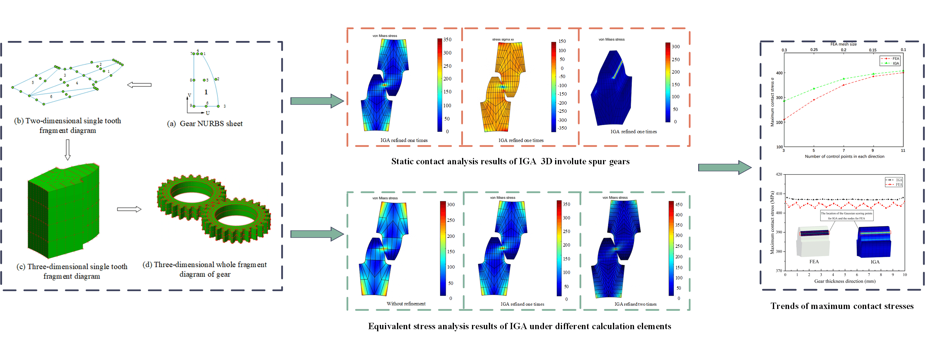
Gears are pivotal in mechanical drives, and gear contact analysis is a typically difficult problem to solve. Emerging isogeometric analysis (IGA) methods have developed new ideas to solve this problem. In this paper, a three-dimensional body parametric gear model of IGA is established, and a theoretical formula is derived to realize single-tooth contact analysis. Results were benchmarked against those obtained from commercial software utilizing the finite element analysis (FEA) method to validate the accuracy of our approach. Our findings indicate that the IGA-based contact algorithm successfully met the Hertz contact test. When juxtaposed with the FEA approach, the IGA method demonstrated fewer node degrees of freedom and reduced computational units, all while maintaining comparable accuracy. Notably, the IGA method appeared to exhibit consistency in analysis accuracy irrespective of computational unit density, and also significantly mitigated non-physical oscillations in contact stress across the tooth width. This underscores the prowess of IGA in contact analysis. In conclusion, IGA emerges as a potent tool for addressing contact analysis challenges and holds significant promise for 3D gear modeling, simulation, and optimization of various mechanical components.Graphic Abstract
Keywords
The gear contact analysis is a complicated nonlinear problem. The classical Hertz formula, first formulated by Hertz [1] in 1881, utilized mathematical and elastic methods to address a variety of contact issues associated with basic shapes and uniform contact surfaces. However, several conditions must be met for the classical Hertz contact method to address certain engineering challenges. Firstly, the traditional finite element analysis (FEA) method for the gear contact problem is to use the
In 2004, isogeometric analysis (IGA) was first proposed by Hughes et al. [2] as an analysis method based on the Non-Uniform Rational B-Splines (NURBS) parametric model to unify the design model and the analysis model and then achieve a seamless connection between design and analysis. The model for IGA is composed of NURBS surfaces or volumes, so the entire model remains smooth, avoiding the problem of inaccurate model representation produced by the standard finite elements’ discrete computational unit densities. By leveraging the NURBS basis, the IGA method avoids the error of the FEA method from the geometric source.
However, despite nearly two decades elapsing since IGA’s inception, its application to complex mechanical components like gears remains limited. Several reasons have contributed to this limitation. One reason is that the complex mechanical parts with many engineering features are very hard to construct to be suitable for IGA. Standard mechanical components, including gears, bearings, bolts, flat keys, splines, and springs, are characterized by specific curves or surfaces. Representing these components as volume parametric solids is far from straightforward. The other reason is that IGA cannot yet work on the analysis tasks under complex work conditions. As a new and promising analysis method to replace the current FEA method, IGA has its gaps. What is more, in using the existing methods of analysis methods some analysis problems remain unsolved. Just as with the problem of gear contact analysis, although there are many analysis methods, including the FEA methods, finding a precise, efficient, economical, and fast analysis method remains to be solved and has attracted many researchers’ interest for decades. The basic idea of IGA is that of using the same mathematical language to express geometric shapes and physical fields. Using a planar NURBS surface or a three-variable NURBS parameter volume as the computational domain, wherein the computational units are the surface or volume units corresponding to the node interval, the NURBS basis function is used as the shape function, and the physical properties of the control vertices are used as the invariant. Therefore, for 3D models with complex structures, the key to successful geometric analysis is to decipher how to build a volume-parameterized model that meets the continuity requirements. To achieve this, it is necessary to solve two problems: the NURBS multi-piece (block) splicing method and boundary continuity coupling. Here, we used IGA to establish the three-dimensional contact model of the gear and compared its tooth profile with that of the standard involute cylindrical gear for geometric error analysis. Then, we developed a new geometric contact analysis algorithm to deal with the frictionless contact problem of 3D gears and compared the analysis results with the results obtained from theoretical calculations and commercial software.
The paper is outlined as follows: In Section 2, an overview of gear contact analysis, isogeometric analysis, and isogeometric contact analysis is presented. In Section 3, a common isogeometric contact analysis for three-dimensional calculations is derived and realized. To study the correctness of calculation formulas and processes, a standard one-fourth semicircle contact model is established, and the results of the isogeometric contact analysis are compared with the Hertz theoretical values and the empirical values from commercial software. In Section 4, a NURBS representation of a gear contact model is analyzed, and the contact Von-Mises stress is obtained and compared with the corresponding values obtained from some commercial software. Section 5 presents the conclusions and ends this paper.
The contributions of our work can be summarized as:
1) The calculation formulas for common 3D isogeometric contact analysis were derived.
2) Based on the requirements for smoothness and continuity of gear contact boundaries, a 3D gear body parameterized model suitable for geometric analysis was constructed using the NURBS multi-block splicing and Nitsche’s method. The correctness and robustness of this method were verified by comparisons with FEA results.
3) The advantages of IGA methods in 3D contact analysis were explored, including the finding that under the same calculation accuracy, there were fewer calculation units and degrees of freedom, smoother expression of contact surfaces, smoother contact stress, and significantly reduced non-physical oscillations.
Gears are some of the most used parts in transmission equipment, so the gear contact problem has gained many researchers’ interest, including other problems such as the fatigue life analysis of gears [3], transmission error analysis of gears [4], and stress analysis of gears [5]. The FEA method has been widely used for the analysis of gears. Li [6] performed a finite element frictionless contact analysis on a three-dimensional gear. Mao [7] used the micro-geometric correction method to reduce the fatigue wear of gear tooth surfaces and calculated the contact stress of gear tooth surfaces with the finite element method. Gonzalez-Perez et al. [8] proposed a method to reduce the calculation cost of the gear meshing by using multi-point constraints at different sections of the gear geometry. Tamarozzi et al. [9] analyzed two gears meshing in an ad-hoc flexible multibody model and proposed an online selection of residual attachment modes for accurate local deformation prediction. Chang et al. [10] calculated the overall deformation of the tooth body by the analytical method and calculated the local deformation in the contact area by the finite element method, which greatly shortened the calculation time. Li [11,12] studied the meshing stiffness and stresses of the straight cylindrical gears by using the finite element method, which considered tooth profile modification, manufacturing errors, and other factors. Wang [13] proposed a method that could correct the tooth profile by using tooth surface contact and established a dynamic model of helical gears. Litvin et al. [14,15] used a gear geometric contact analysis technology to modify the tooth surface of helical gears in three dimensions and reduce the amplitude of transmission error, and also developed a six-degree-of-freedom helical gear dynamic model to study the time-varying meshing stiffness (TVMS) calculation method by considering axial deformation. Lin et al. [16] proposed a transmission error analysis method for helical gear systems that considered machining assembly and correction errors, and established a bent-twist shaft coupling dynamic model for the analysis and control of gear system vibration and noise.
Since Hughes et al. [17] proposed the IGA method, many researchers have further developed it. Currently, this method has been applied in many fields, such as heat conduction problems [18], fluid flow problems [19,20], acoustic problems [21], electromagnetic problems [22], and fluid structure coupling problems [23–28]. IGA has also been applied in the medical domain [29–30].
IGA has been deeply and widely verified in the field of mechanical engineering. The most obvious advantage of the IGA method is its geometric accuracy, which can accurately express the geometric model. By bonding complex models with multiple NURBS surfaces, Kiendl et al. [31,32] solved the continuity problem between multiple NURBS surfaces. Based on the advantages of IGA, it has been applied to plate and shell analysis by many researchers. To study the vibration of thin-walled beams, Carminelli et al. [33] used B-splines as elements in establishing the thin-walled shell elements of multi-layer composite materials. Uhm et al. [34] used T-splines to establish a plate and shell model for IGA, and effectively solved the problem of the degree of freedom that could not be rotated at the control points. Hirschler et al. [35] proposed a dual-domain decomposition algorithm to accurately analyze the unqualified polyhedral Kirchhoff-Love shells. Jamires et al. [36] proposed an IGA-based method to study the stability of laminates and shallow shells. The proposed method was applied to the stability analysis of various examples and obtained excellent results. Norouzzadeh et al. [37] applied the IGA method to the dynamic analysis of the shell and used the method to generate the geometry of the surface area and the approximate displacement field in the shell.
The IGA method has also been combined with other research methods to solve broader problems. Chen et al. [38] realized a parametric optimization for complex structural shapes by using IGA and verified the effectiveness of this method with several complex planar shapes. Xia et al. [39] proposed a coupling model based on IGA and bond-ed peridynamics (PD) (IGA-PD) and proved that in the IGA-PD coupling model, the PD node could be constructed by the control network of IGA, which improved the calculation accuracy and efficiency of crack problems and provided a solution method for crack problems with an accurate geometric model. Aung et al. [40] combined shape optimization with IGA and applied this method to the analysis and optimization of welds. The analysis and optimization results showed that the stress concentration of welds was greatly reduced by using this method.
Since the gear is a typical part in mechanical engineering, here, we give a detailed overview. Yusuf et al. established a three-dimensional gear model with NURBS to study the strength and deformation of a gear tooth under load. By comparing the results of IGA with the corresponding values of the Lewis equation and FEA, it was proved that the IGA model could obtain more accurate gear analysis results. However, the authors only gave the result of stress analysis of a single tooth, instead of the teeth that kept contact. In addition, the established IGA gear model was not compared with the standard gear model for the geometric error of the tooth profile. As there is no specific derivation formula for the analysis of isogeometric gears [41]. Considering the mesh interference and profile modification under loads, Beinstingel et al. used NURBS to design an accurate tooth profile to explore the influence of mesh density on gear meshing stiffness matrix, then proved that the analysis established by IGA had good applicability and stability. However, the influence of the stiffness matrix derived under the quasi-static state on the gear force was not discussed [42].
For the contact analysis between mechanical parts, some researchers have also conducted relevant research with IGA. To quickly search for the control points on isogeometric models, Stadler et al. [43] proposed an efficient search algorithm for adaptive fine mesh on adjacent elements search. Temizer et al. [44] used the NURBS contact discretization node-to-surface (KTS) algorithm to study frictionless contact problems. It qualitatively showed that the application of this algorithm could improve the analysis accuracy and convergence, which focused on the effect of the proposed new algorithm on mesh discretization without analyzing its stress results. Lu [45] was the first to develop the IGA algorithm framework for contact problems. Two contact algorithms were used to analyze Hertz and interference contact examples, and the analytical solutions were compared. Mathisen et al. [46] simulated the large deformation contact problem between pipeline and trawl gear based on the IGA of mortar, and the numerical example demonstrated that isogeometric surface discretization delivered more accurate and robust predictions of the response compared to Lagrange discretization. Based on the local maximum entropy (LME) approximation, Greco et al. [47] explored the simulation of small deformation contact problems with a coupled isogeometric meshless formulation. Kamensky et al. [48] used IGA to derive the contact equation based on volume potential energy and used the structural mechanics of the atrioventricular valve to illustrate the validity of this equation. Emad et al. [49] proposed an adaptive method to deal with contact problems. The effectiveness of this method was verified by the Hertz problem and three hyperelastic contact problems, and the results showed that IGA had good convergence not only for contact pressure, but also for the limit of contact area.
In summary, although isogeometric analysis has obvious advantages in geometric accuracy, more work is needed to effectively utilize IGA in solving the problems of gears:
1) There is no specific mechanical formula for the meshing contact of two cylindrical gears combined with the theory of isogeometry.
2) Compared with the FEA method, the advantages of the IGA method in modeling and analyzing two cylindrical gears are not clear.
3 Realization of Isogeometric Contact Analysis
The process of IGA is similar to FEA, but there are also differences. For instance, while FEA uses the Lagrangian Function as its basis function, and the boundary of the model can only reach
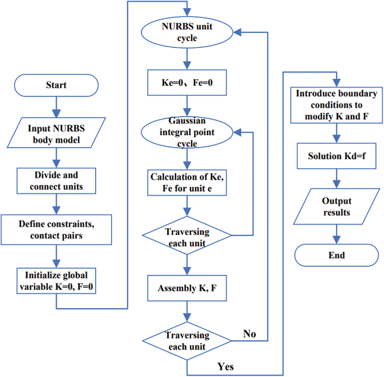
Figure 1: Process of isogeometric contact analysis
3.1 Search of the Contact Areas
Since the isogeometric model was presented with NURBS, searching the contact areas meant searching the control points. So, the searching operation was divided into two steps. The first step, called a global search, was to determine which elements would be contacted, and the second step called local search was to determine the contact control points on the contacted units. The difficulty lay in the local search step. As shown in Fig. 2, the spatial distance function S required the shortest distance from the spatial point to the surface.
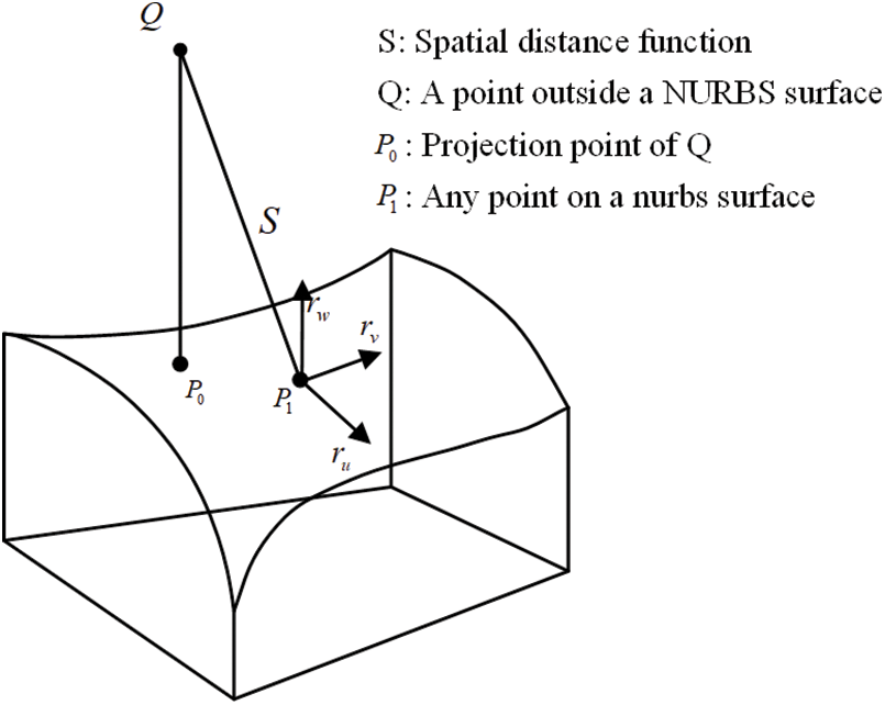
Figure 2: Distance from a space point to a surface
As shown in Fig. 2, given a point
where,
The equation was solved as:
After calculation, the node vector was updated for calculation by:
Finally, the calculation error
When the given conditions were met, the point
From the given conditions it was obtained that:
Newton’s method was used to solve Eq. (7), and the corresponding iterative equation was:
where,
3.2 Treatment of Constraints and Loads
When dealing with contact constraints, numerical solutions should be carried out. The widely used penalty function method is used to calculate the contact force [52], however, this method does not increase the degree of freedom in the numerical solution and does not change the scale of the matrix [53]. The penalty factor introduced by the penalty function was multiplied by the penetration of the contact interface to calculate the contact force. In fact, the contact problem was transformed into a material problem to solve, and the specific calculation formula was expressed as:
where,
The equation was rewritten by variation:
According to Eq. (6), Eq. (13) was rewritten as:
Since the contact surfaces of A and B were composed of NURBS surfaces, we could set:
where,
Assuming that the set of Gauss points on the contact area was defined as
where,
In this way, the projection of the contact force at the control point was obtained as:
The three-dimensional contact stiffness matrix was expressed as:
where,
Suppose that:
Newton’s method was used to solve the differential equation, and the iterative formula was:
where
The variation of Eq. (23) was obtained as:
To obtain the stiffness matrix [54], it was necessary to further deduce and perform first-order Taylor expansion on
Eq. (27) was obtained by variation as:
Substituting Eq. (28) into Eq. (26), we obtained:
Combined with the Jacobian matrix
The NURBS discretization of the above formula was obtained:
So, the terms in Eq. (21) were gotten as:
Then, the contact matrix
where,
After obtaining the stiffness matrix, the equilibrium equations of the contact system were obtained, which can be expressed in matrix form as:
where,
Then, the element stiffness matrix was written as:
After the element stiffness matrix was obtained, the overall stiffness matrix
where,
where,
Although isoparametric elements are used in isoparametric geometry, the mapping relationships among parent elements coordinate, physical coordinate, and parameter coordinate need to be carried out in IGA [55]. The parent element refers to the Gaussian integral domain. As shown in Fig. 3,
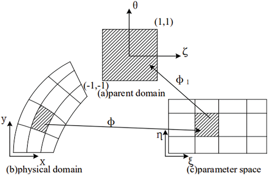
Figure 3: Mapping among domains
The determinant of Jacobian transformation corresponding to the transformation from parameter coordinate to parent unit coordinate is:
The Jacobian transformation matrix corresponding to the transformation from physical unit coordinate to parameter space coordinate is:
Therefore, the Jacobian determinant of the mapping from the parent unit to the physical unit was obtained as:
The expression of the element stiffness matrix was:
where,
3.3 Hertz Contact Example Validation
For the Hertz contact problem, this subsection gives the geometric settings and boundary conditions of the Hertz contact model, calculates the analytical expression of the Hertz contact problem, and compares it with the FEA models with different mesh densities to verify the correctness of the equivalent geometric contact algorithm.
3.3.1 Theoretical Value of the Hertz Contact Model
In 1881, Hertz obtained the formulas required for calculating the contact problem according to the mathematical linear elasticity method and gave the following assumptions: Each object is regarded as an elastic, uniform and isotropic half space, which is loaded on a small elliptical region of its smooth surface. Assuming that the surface has no friction, its contact area must be smaller than the surface radius and object size, and the geometry of the contact interface is described by quadratic polynomial. The Hertz contact model is shown in Fig. 4.
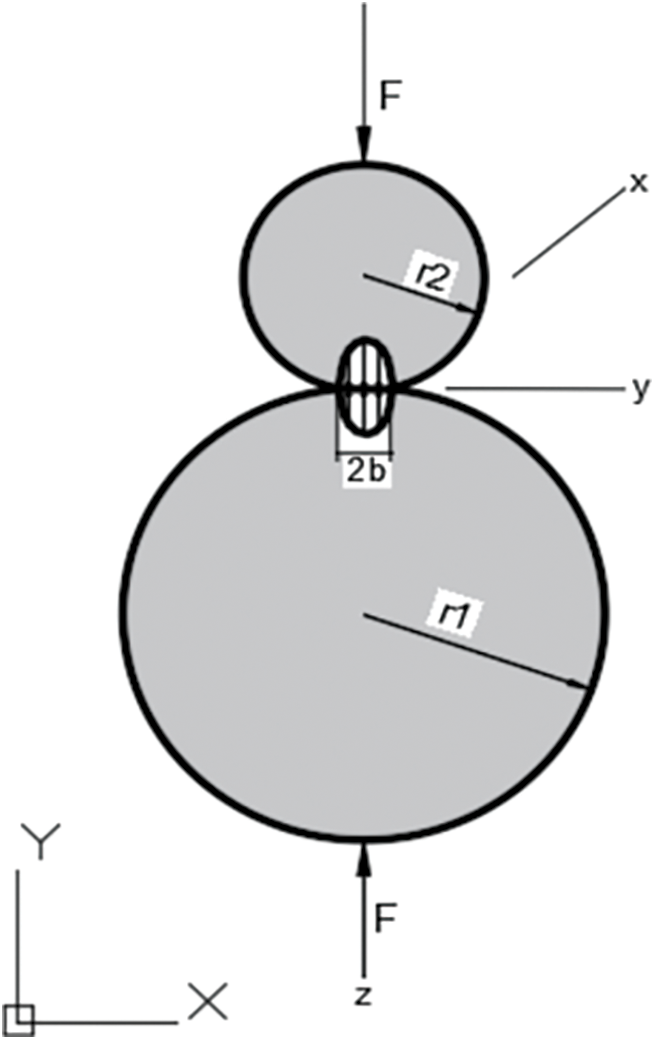
Figure 4: Hertz contact model
The analytical solution of the half width b of the contact area was obtained from Eq. (46).
As evident from Eq. (46), the value of half width
Considering the symmetry of the model, a quarter model could be established to save on calculation costs. The radius of the two cylinders was 2 mm, the thickness was 5 mm, and the Neumann boundary condition F was 1000 N. To reduce the influence of simplifying the mechanical model, the constant Dirichlet boundary condition v = 0.001125 was used to replace the Neumann boundary condition F at the top of the cylinder [49]. The penalty function method was used for contact analysis, and the penalty value is 1000E. According to Eqs. (46) and (47), the Hertz contact theoretical value was calculated as: the contact half width b = 0.0237 mm and the maximum contact stress value was 735 MPa. The Hertz contact analysis model and calculation parameters are shown in Fig. 5.
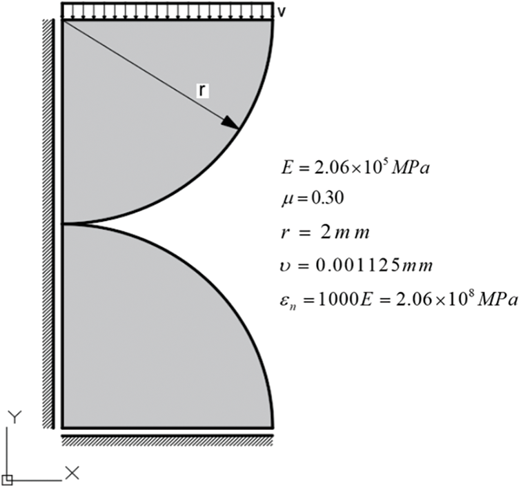
Figure 5: Hertz contact analysis model
3.3.2 Hertzian Contact Values Calculated by IGA and FEA
To fully verify the accuracy of the isogeometric contact analysis, the isogeometric Hertz contact analysis and FEA were carried out concurrently. The advantages of the concurrent analysis were mainly reflected in that it allowed a visual determination of whether the 3D isogeometric contact theory and procedure could pass the Hertz contact test, and additionally, by adjusting the computational unit densities and comparing it with FEA, the differences or advantages between the results of IGA and FEA under different computational unit densities were explored. The isogeometric Hertz contact model used NURBS body with order 2 in
The selection of FEA contact settings and solvers had a significant impact on the analysis results. The commercial finite element software selected in this article was Ansys Workbench. For contact settings, the contact surfaces of the upper and lower half cylinders were selected for contact and target surfaces, respectively; select Contact Type as Frictionless. The penetration tolerance was set to 0.001, the penalty function value was 10E, and the contact offset value was 0 mm. The “Contact Geometry Correction” and “Target Geometry Correction” options were disabled. The rest were default settings. At the Solver setup, the Iteration method selection was the Newton-Raphson method; the residual value was 10E-6, and the rest were default settings.
Generally, the more accurate calculation results were due to the large number of calculation units. Therefore, the IGA results with the node vector {0 0 0 0 0.0625 0.125 0.1875 0.25 0.3125 0.375 0.4375 0.5 0.5 0.5625 0.625 0.6875 0.75 0.8125 0.875 0.9375 1 1 1} were compared with the FEA results with the mesh size of 0.05 mm. The results are shown in Fig. 6, where Fig. 6a shows the results of equivalent stress distribution, Fig. 6b shows the results of stress distribution in Y–direction, and Fig. 6c shows the results of contact stress distribution.
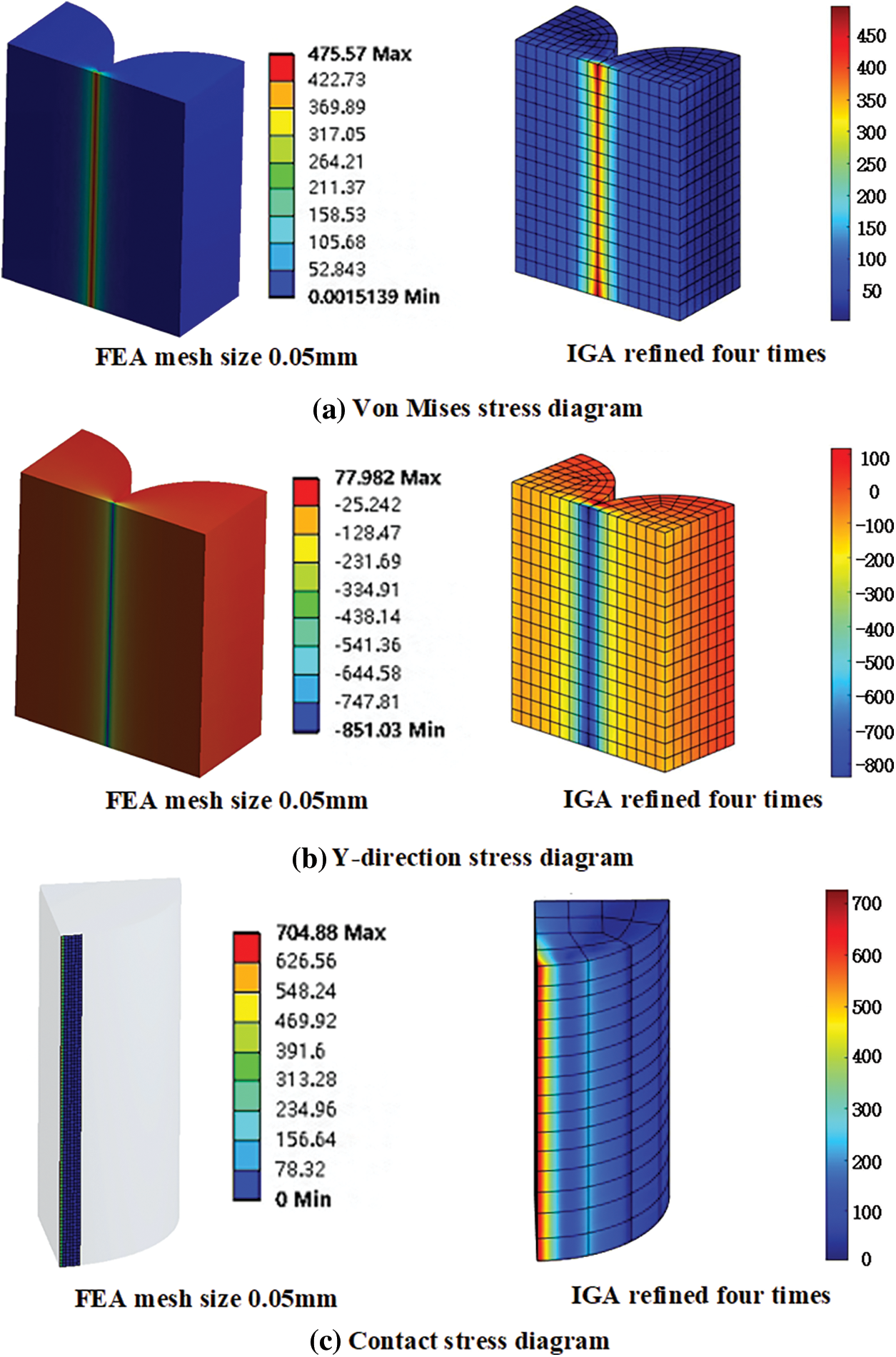
Figure 6: Comparison of IGA and FEA Hertz contact model analysis results
According to the Hertz contact theory value, the maximum contact stress of the two columns was 735 MPa. From the analysis results in Fig. 6c, the maximum contact stress calculated by FEA was 704.88 MPa, and the maximum contact stress calculated by IGA was 719.27 MPa. The results of IGA and FEA were close to the theoretical value in the case of dense calculation elements. Figs. 6a and 6b show that the maximum equivalent force and maximum Y-directional stress in the FEA results were 475.57 MPa and −857.03 MPa, while the maximum equivalent force and maximum Y-directional stress in the IGA results were 482.43 and −866.32 MPa, respectively. In terms of stress distribution, the results of IGA and FEA had approximately the same trend of stress distribution.
To compare the effect of computational unit densities on the analysis results, the contact stresses of isogeometric and finite element models with different mesh densities were studied, the boundary effect on the contact stress was also eliminated, and the contact stress at the contact position of the cross-section in the half thickness direction was selected and compared with the Hertz contact theory value. Fig. 7 shows the maximum contact stress values calculated by IGA and FEA at different computational unit densities and compares the maximum contact stress value with the maximum Hertz contact theoretical value.
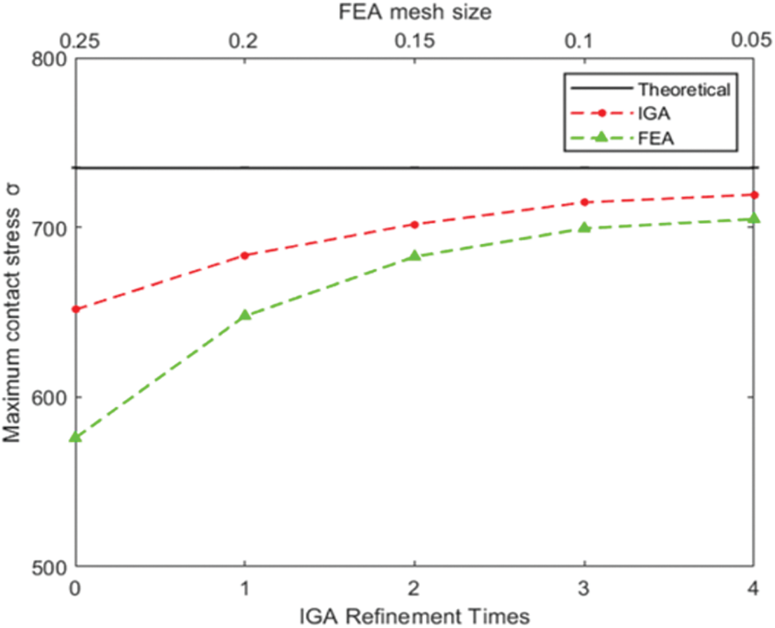
Figure 7: Convergence of maximum contact pressure between FEA and IGA
As shown in Fig. 7, with the increase in calculation elements, the IGA and FEA results converged to the theoretical value. Compared with the FEA, the isogeometric contact analysis program obtained higher calculation accuracy with fewer calculation elements, and the increase of calculation elements seemed to have less impact on the results of IGA. The isogeometric models with five computational unit densities were compared with the element and node data of the finite element model, as presented in Table 1.
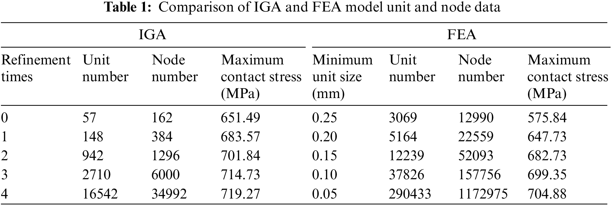
Under the same calculation accuracy, the number of elements used in the isogeometric contact analysis was less. Taking the 4× refinements as an example, the number of IGA units was only 34,992, while the number of FEA units was 290,433, which was eight times the number of IGA units. The accuracy of IGA was less affected by the density of computational units and converged more easily than the finite element method. Fig. 8 shows the comparison between the results of the geometric contact stress distribution of the refined 2, 3, and 4 contact width areas and the Hertz contact theoretical value, which also showed that the accuracy of the geometric analysis was less affected by the element density.
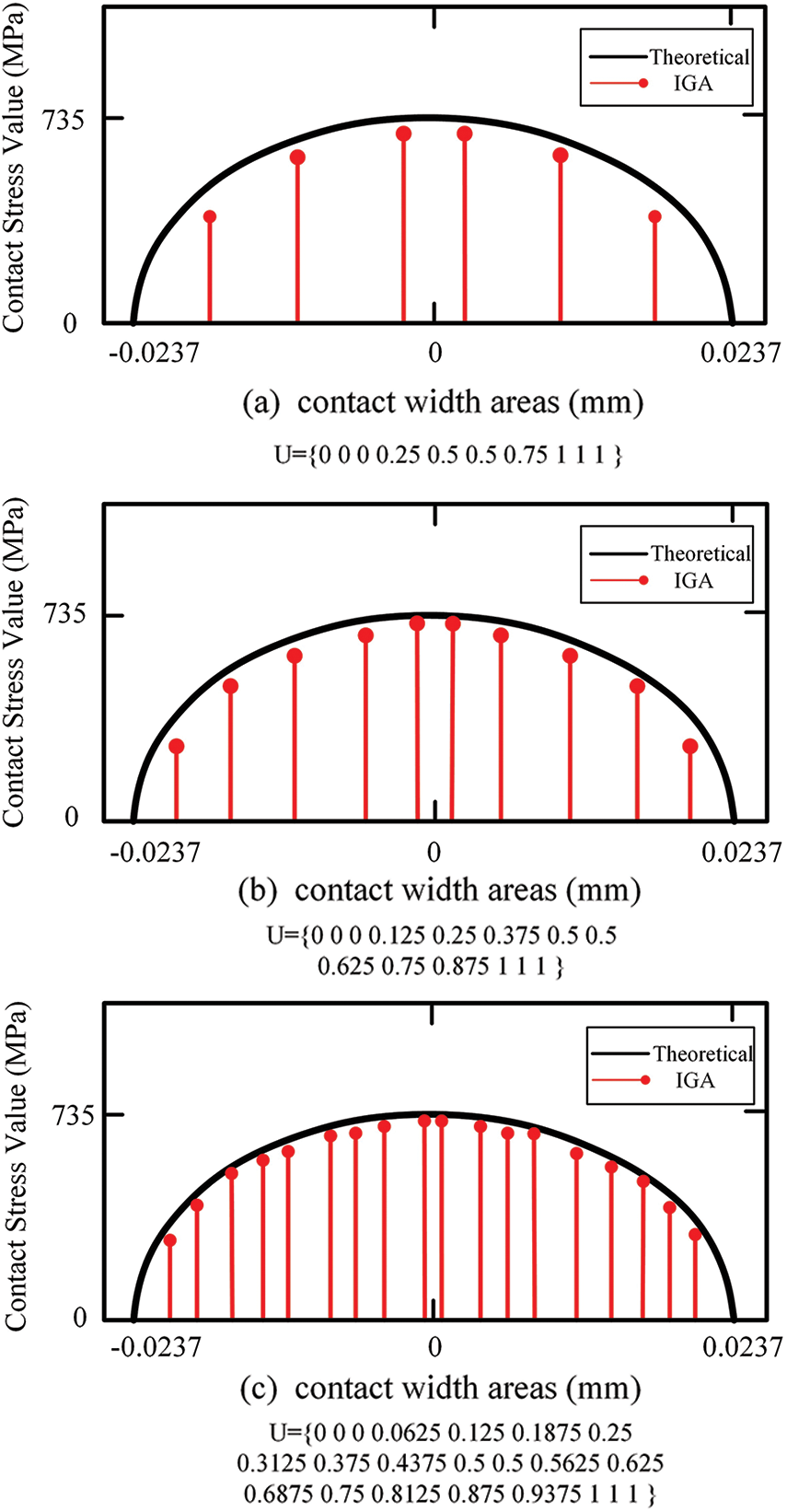
Figure 8: Contact stress distribution in contact width region
In summary, the IGA contact algorithm in this paper passed the Hertz contact test. Compared with the FEA method, under global refinement, the IGA contact algorithm had fewer nodal degrees of freedom and computational units with the same computational accuracy, and the analytical accuracy was less affected by the computational unit density, which was easier to converge.
4 Isogeometric Contact Analysis for Gears
Compared with the traditional FEA method, the IGA method has the greatest advantage of using the same geometric model representation in modeling and analysis, which can eliminate the discrete error and effectively avoid the discrete approximation problem of the finite element model. Additionally, the boundary of the IGA model can be at least
where,
4.1 3D Involute Spur Gear Parametric Multi Piece Modeling
The main design parameters of the gear in this paper were module
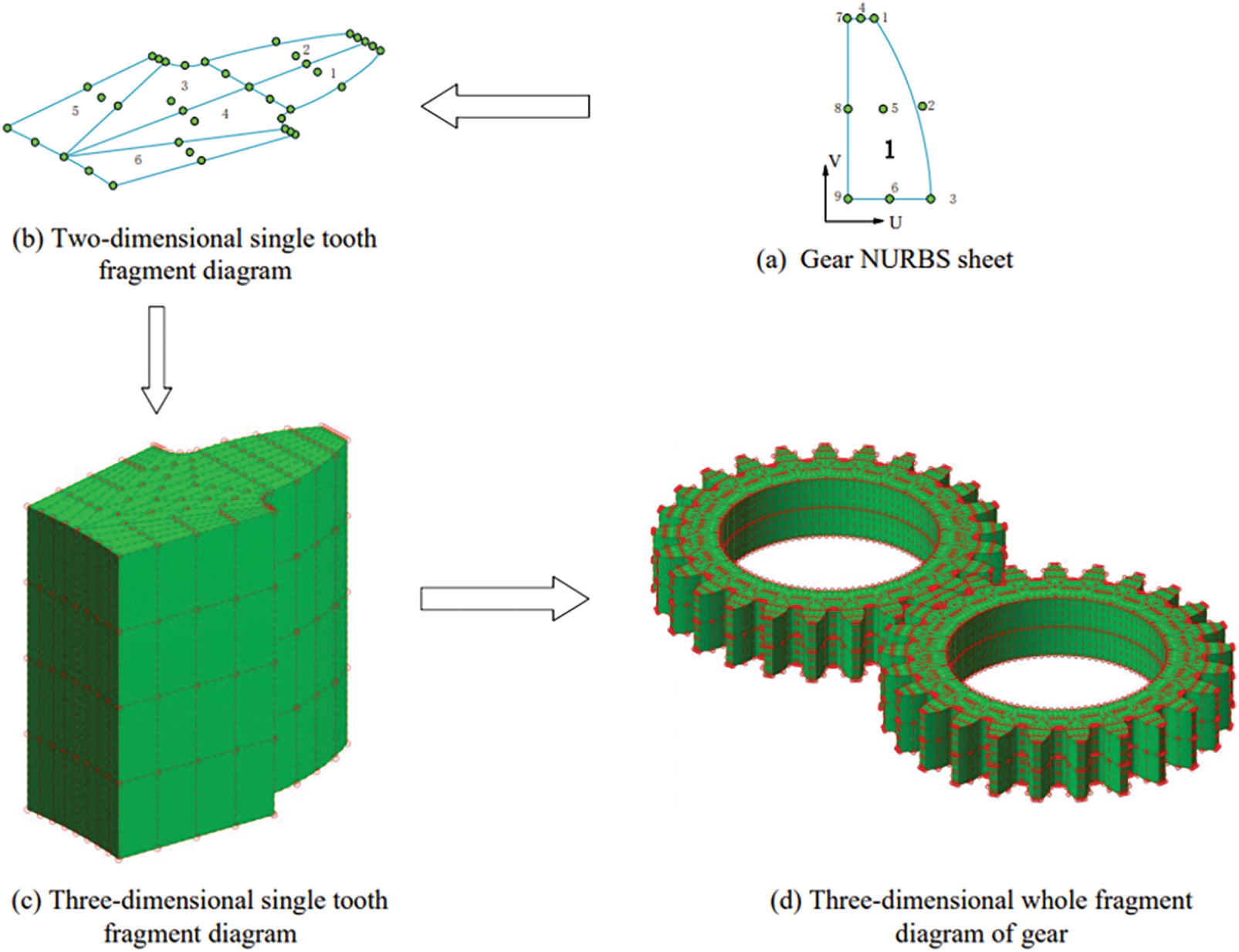
Figure 9: 3D involute straight tooth body parametric multi-piece modeling process
As shown in Fig. 9, the 3D involute spur gear adopted the multi-piece suture modeling method [56], and a pair of gears with the same size were meshed with each other. To ensure continuous and smooth contact areas, it was required that the contact surface of the gear be composed of a single NURBS block. With single tooth contact, the second patch could be obtained by the mirror operation of the first patch, and the two adjacent patches shared the control points on the coincident edges. Each tooth was stitched by six NURBS surface patches. According to the design calculation method, all six patches of a tooth were constructed. Then the plane single tooth model was stretched along the vertical direction, with the stretching length of 10 mm, as shown in Fig. 9c. The parameters corresponding to NURBS were set as follows: the node vector
In the process of 3D gear modeling, this paper used the Nitsche’s method to deal with the continuity problem between the NURBS multi-sheets (blocks), achieving consistent parameterization of patch interfaces between multi-sheets (blocks) to ensure that the established multi-sheets (blocks) gear model could be used for IGA. The implementation process was:
1. Solve the stiffness matrix of a single NURBS patch (block).
2. Use Gaussian scoring point mapping on discontinuous boundaries.
3. Use Nitsche’s method to calculate the coupling stiffness matrix of discontinuous boundaries.
4. Combine the coupling stiffness matrix and the stiffness matrix of a single NURBS patch (block) into the global stiffness matrix.
Nitsche’s method weak form:
Define
The standard application of Nitsche’s method for the coupling was: Find
For all
Fig. 10 shows the local boundary comparison between the IGA model and FEA gear. Obviously, the boundary of IGA model could be fully expressed with fewer calculation units, the boundary was more continuous and smooth, and the calculation units were at least
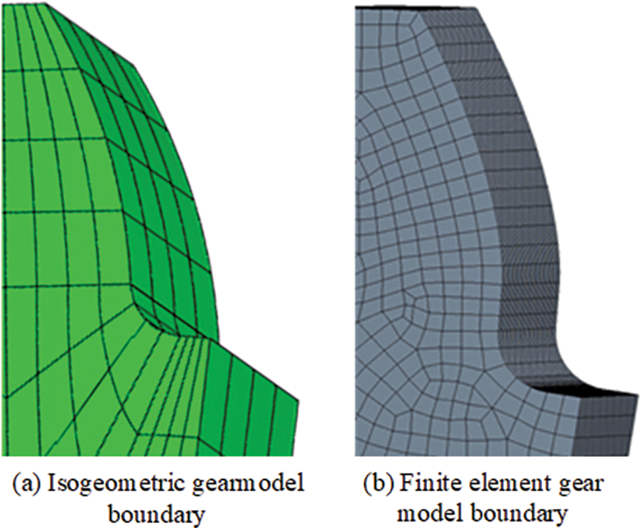
Figure 10: NURBS gear body model boundary and finite element discrete boundary
4.2 Mechanical Model Equivalence
Similar to the FEA, in the process of applying boundary conditions, in the IGA it is difficult to directly apply mechanical boundary conditions and displacement boundary conditions such as torque and rotation angle, which need to be equivalent to control point force and displacement. Fig. 11 shows the equivalent principle of the mechanical model for static contact analysis of 3D involute spur gears.
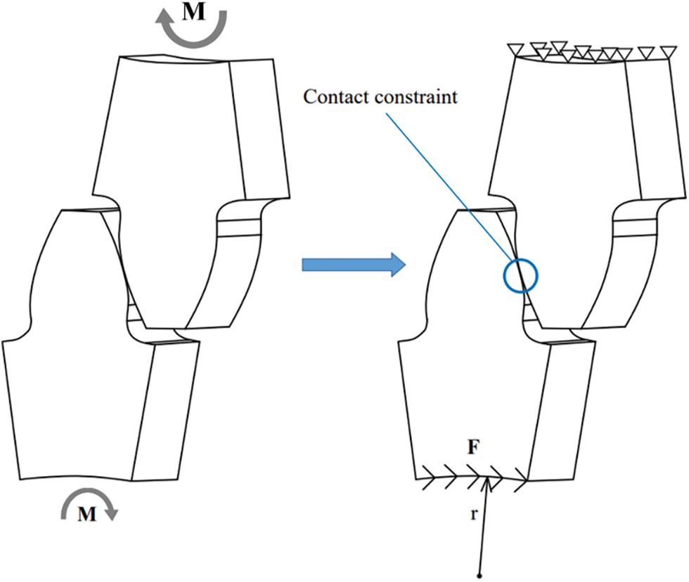
Figure 11: 3D involute straight tooth static contact analysis mechanical model equivalent
In the original working condition, the two meshing gears are meshed under the action of torque
That is, regardless of the displacement of the lower gear, the distance from the contact surface between the gear and the shaft to the centerline of the gear shaft was constant. The penalty function method was used to solve the coupling boundary condition problem, and the penalty value was 1000E. Secondly, the torque
Thirdly, the surface force
Finally, the mechanical model equivalence of the 3D involute single tooth static contact analysis was completed.
To verify the accuracy of static contact analysis of 3D involute spur gears, two different methods, IGA and FEA, were used to analyze the mechanical model. Fig. 12 shows the finite element calculation results of two times equal geometric refinements (i.e., the node vector in one direction is {0 0 0 0.25 0.5 0.5 0.75 1 1 1} and the element size was 0.2 mm under global refinements. Among them, Fig. 12a shows the equivalent stress distribution, Fig. 12b shows the
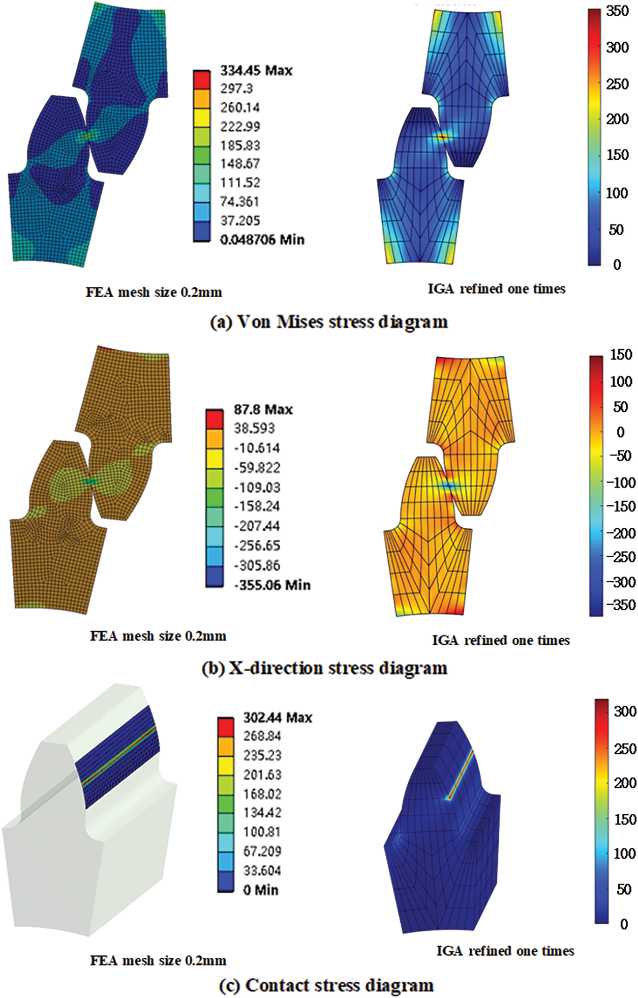
Figure 12: Static contact analysis results of IGA and FEA 3D involute spur gears
As evident from Fig. 12, under a certain calculation unit density, the results of IGA were highly similar to those of FEA in terms of numerical size, physical field distribution, stress concentration area, etc. The maximum equivalent force in IGA was 347.82 MPa while the maximum equivalent force in FEA was 334.45 MPa. The maximum contact stress in IGA was 318.61 MPa, and the maximum contact stress in FEA was 302.44 MPa. The IGA obtained numerical results close to FEA with fewer nodes and elements, and its stress distribution was also roughly the same, which verified the feasibility of equal geometric contact analysis.
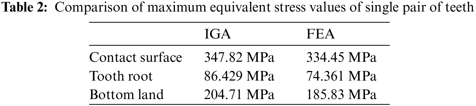
The analysis results showed that the equivalent force of a single pair of teeth was mainly concentrated at the meshing surface, tooth root, and tooth groove bottom surface, and the maximum value was located at the meshing point. The distribution of the maximum equivalent force at different locations is shown in Table 2.
In order to consider the influence of unit density on the calculation accuracy, three types of NURBS volume models with different unit density were obtained by adjusting the refinement times, and the
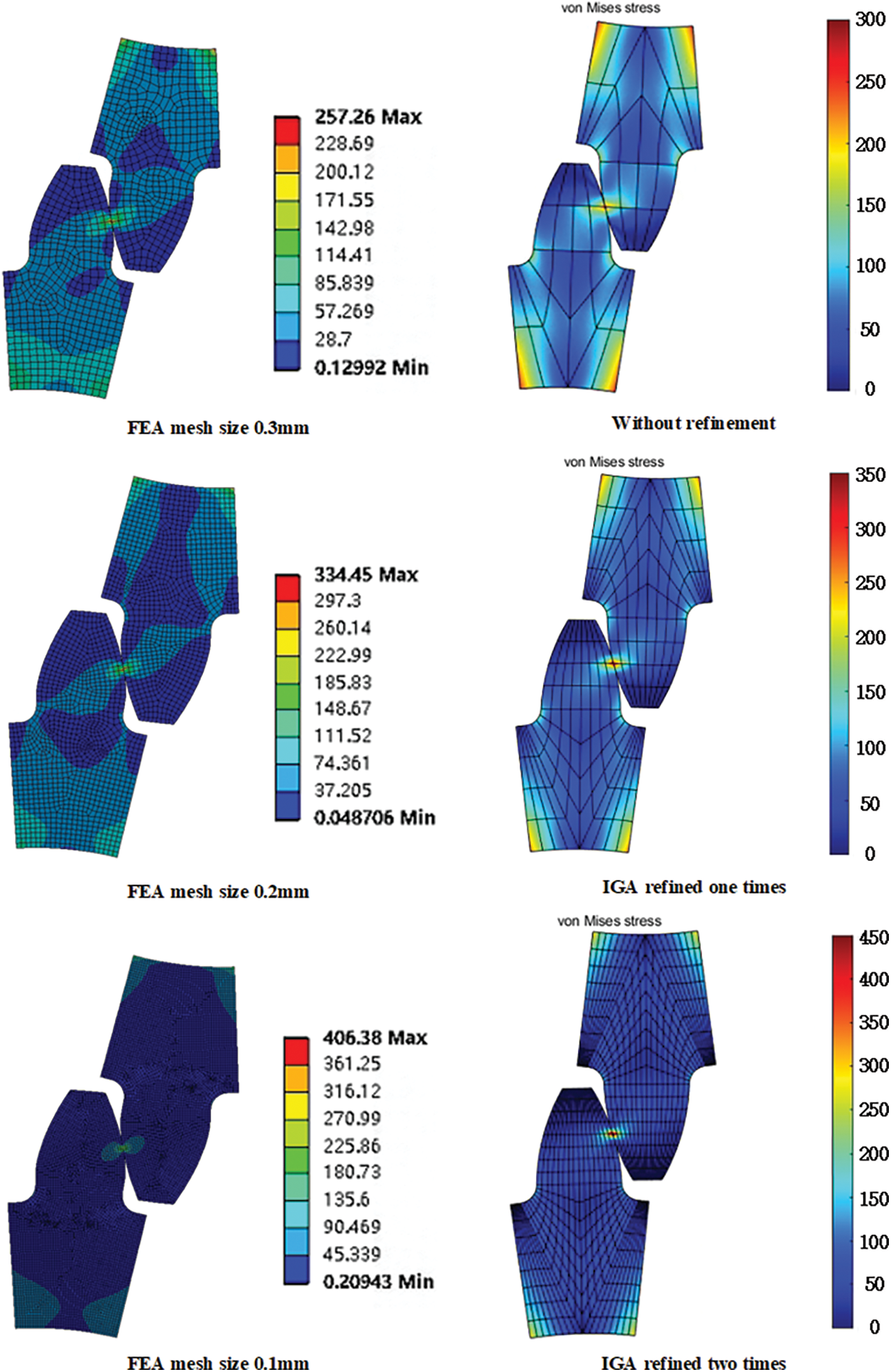
Figure 13: Equivalent stress analysis results of isogeometric and finite element under different element densities
As shown in Fig. 13, the equivalent stress results and distribution of IGA showed the same law as that of FEA, and with the gradual increase of calculation element density, the peak area of equivalent stress gradually concentrated on the gear meshing point and the bottom surface of the tooth groove. From the numerical change analysis of the maximum equivalent stress, the FEA results increased from 257.25 to 406.38 MPa, while the IGA results increased from 300 to 450 MPa. Although it was difficult to judge the analysis accuracy from the maximum equivalent stress increase after refinement of the calculation elements, it was evident that even with sparse calculation elements, the IGA results still had high accuracy.
The maximum contact stress of IGA with different numbers of refinements and the maximum contact stress of FEA with different unit sizes were extracted for trend fitting to compare and analyze the variation of the maximum contact stress with the density of calculated units. Fig. 14 shows the trend of the maximum contact stress of IGA and FEA under different unit densities.
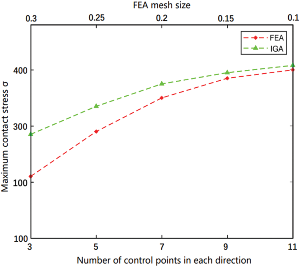
Figure 14: Trends of maximum contact stresses in IGA and FEA at different calculated unit densities
As evident from Fig. 14, from the perspective of the development trend of the maximum contact stress of a single tooth, the IGA and FEA both showed the same law; with the increase of the calculation unit density, the maximum contact stress gradually increased and tended to converge. Compared with the FEA, the IGA was observed to have relatively high calculation accuracy with fewer calculation units, which is the advantage of IGA.
Fig. 15 shows the distribution of maximum contact stress in the direction of single tooth width of IGA with two times refinements, unidirectional node vector {0 0 0 0.25 0.5 0.75 1 1 1}, and FEA with element mesh size of 0.1 mm. Compared with FEA, the distribution of the maximum contact stress in the width direction of an IGA single tooth was more stable with less fluctuation, indicating that the false vibration of the contact stress in the width direction of IGA was less and the contact search was unique. In contrast, during the FEA, the contact stress obviously oscillated in the direction of tooth width, which was due to the influence of the Lagrange interpolation function. The elements were
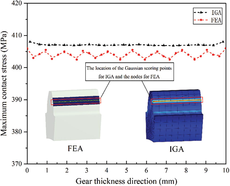
Figure 15: Distribution of maximum contact stress of IGA and FEA along gear thickness
In this paper, the 3D isogeometric contact theoretical analysis formula was derived, with the algorithm subsequently applied to the involute spur gear meshing contact analysis. Upon comparison with the FEA results, the validity of the isogeometric contact analysis outcomes was confirmed, leading to the following conclusions:
1. At a certain density of calculation units, the results of IGA were highly similar to those of FEA in numerical size, physical field distribution, and stress concentration area.
2. As the density of calculation units increased, the FEA results (such as equivalent force and contact stress) changed markedly, while the IGA results had a smaller amplitude of change.
3. Although it was difficult to judge the analysis’ accuracy from the increases in the analysis results (such as equivalent force and contact stress) after the increase of the calculation unit density, we have to admit that even if the calculation unit density was sparse, the IGA results still had high accuracy.
4. By comparing the distribution of the maximum contact stress in gear width direction, the results of the IGA fluctuated less, and were more uniform, indicating that in the IGA, the calculation units were high-order continuous, the contact normal was unique, and the non-physical vibration of the contact stress was not substantial, which are the advantages of the IGA.
Nonetheless, it is acknowledged that there is room for optimization in the employed code because of its longer calculation time than that of some commercial software. Addressing this optimization challenge is a forthcoming endeavor.
Acknowledgement: This research was supported by the National Natural Science Foundation of China and the Shanghai Municipal Commission of Science and Technology. Additionally, the authors express their sincere gratitude to the reviewers for their valuable comments, which have greatly improved this paper.
Funding Statement: The authors gratefully acknowledge the support provided by the National Nature Science Foundation of China (Grant Nos. 52075340, 51875360) and Project of Science and Technology Commission of Shanghai Municipality (No. 19060502300).
Author Contributions: The authors confirm contribution to the paper as follows: study conception and design: Long Chen, Zhonghou Wang; data collection: Long Chen, Yan Yu, Yanpeng Shang; analysis and interpretation of results: Yanpeng Shang, Yan Yu; draft manuscript preparation: Zhonghou Wang, Long Chen, Yan Yu; supervision: Long Chen, Zhonghou Wang, Jing Zhang. All authors reviewed the results and approved the final version of the manuscript.
Availability of Data and Materials: The data underlying this article will be shared on reasonable request from the corresponding author.
Conflicts of Interest: The authors declare that they have no conflicts of interest to report regarding the present study.
References
1. Hertz, H. (1882). Ueber die Berührung fester elastischer Körper. Journal für die Reine und Angewandte Mathematik, 1882(92), 156–171. [Google Scholar]
2. Hughes, T. J. R., Cottrell, J. A., Bazilevs, Y. (2005). Isogeometric analysis: CAD, finite elements, nurbs, exact geometry and mesh refinement. Computer Methods in Applied Mechanics & Engineering, 194(39–41), 4135–4195. [Google Scholar]
3. Deng, X. (2019). Analysis and prediction of gear fatigue life. IOP Conference Series: Earth and Environmental Science, 252, 22–24. [Google Scholar]
4. Tak, S. H., Hwang, G. S., Son, Y. S., Bae, H. J., Lyu, S. K. (2007). A study on the transmission error of the gear on contact load. Journal of the Korean Society of Tribologists and Lubrication Engineers, 23(3), 117–122. [Google Scholar]
5. Li, Z., Chen, Y. (2013). The stress analysis on spur gear meshing simulation. Applied Mechanics and Materials, 392, 151–155. [Google Scholar]
6. Li, S. (2002). Gear contact model and loaded tooth contact analysis of a three-dimensional, thin-rimmed gear. Journal of Mechanical Design, 124(3), 511–517. [Google Scholar]
7. Mao, K. (2007). Gear tooth contact analysis and its application in the reduction of fatigue wear. Wear, 262(11–12), 1281–1288. [Google Scholar]
8. Gonzalez-Perez, I., Fuentes-Aznar, A. (2017). Implementation of a finite element model for stress analysis of gear drives based on multi-point constraints. Mechanism and Machine Theory, 117, 35–47. [Google Scholar]
9. Tamarozzi, T., Ziegler, P., Eberhard, P., Desmet, W. (2013). Static modes switching in gear contact simulation. Mechanism and Machine Theory, 63, 89–106. [Google Scholar]
10. Chang, L., Liu, G., Wu, L. (2015). A robust model for determining the mesh stiffness of cylindrical gears. Mechanism and Machine Theory, 87, 93–114. [Google Scholar]
11. Li, S. (2015). Effects of misalignment error, tooth modifications and transmitted torque on tooth engagements of a pair of spur gears. Mechanism and Machine Theory, 83, 125–136. [Google Scholar]
12. Li, S. (2007). Effects of machining errors, assembly errors and tooth modifications on loading capacity, load-sharing ratio and transmission error of a pair of spur gears. Mechanism and Machine Theory, 42(6), 698–726. [Google Scholar]
13. Wang, C. (2019). Optimization of tooth profile modification based on dynamic characteristics of helical gear pair. Iranian Journal of Science and Technology, Transactions of Mechanical Engineering, 43(Suppl 1), 631–639. [Google Scholar]
14. Litvin, F. L., Gonzalez-Perez, I., Fuentes, A., Hayasaka, K., Yukishima, K. (2005). Topology of modified surfaces of involute helical gears with line contact developed for improvement of bearing contact, reduction of transmission errors, and stress analysis. Mathematical and Computer Modelling, 42(9–10), 1063–1078. [Google Scholar]
15. Litvin, F. L., Fuentes, A., Gonzalez-Perez, I., Carvenali, L., Kawasaki, K. et al. (2003). Modified involute helical gears: Computerized design, simulation of meshing and stress analysis. Computer Methods in Applied Mechanics and Engineering, 192(33–34), 3619–3655. [Google Scholar]
16. Lin, T., He, Z. (2017). Analytical method for coupled transmission error of helical gear system with machining errors, assembly errors and tooth modifications. Mechanical Systems and Signal Processing, 91, 167–182. [Google Scholar]
17. Bazilevs, Y., Beirao da Veiga, L., Cottrell, J. A., Hughes, T. J., Sangalli, G. (2006). Isogeometric analysis: Approximation, stability and error estimates for h-refined meshes. Mathematical Models and Methods in Applied Sciences, 16(7), 1031–1090. [Google Scholar]
18. Chen, X., Yin, X., Li, K., Cheng, R., Xu, Y. et al. (2021). Subdivision surface-based isogeometric boundary element method for steady heat conduction problems with variable coefficient. Computer Modeling in Engineering & Sciences, 129(1), 323–339. https://doi.org/10.32604/cmes.2021.016794 [Google Scholar] [CrossRef]
19. Rodrigues, J. A. (2020). Isogeometric analysis for fluid shear stress in cancer cells. Mathematical and Computational Applications, 25(2), 19. [Google Scholar]
20. Rasool, R., Corbett, C. J., Sauer, R. A. (2016). A strategy to interface isogeometric analysis with Lagrangian finite elements-Application to incompressible flow problems. Computers & Fluids, 127, 182–193. [Google Scholar]
21. Lee, W., He, J., Guo, J. (2011). The collocation multipole method for acoustic problems with elliptical boundaries. The International Conference on Computational & Experimental Engineering and Sciences, 18(3), 65–66. [Google Scholar]
22. Garcia, D., Pardo, D., Calo, V. M. (2019). Refined isogeometric analysis for fluid mechanics and electromagnetics. Computer Methods in Applied Mechanics and Engineering, 356, 598–628. [Google Scholar]
23. Heltai, L., Kiendl, J., DeSimone, A., Reali, A. (2017). A natural framework for isogeometric fluid-structure interaction based on BEM-shell coupling. Computer Methods in Applied Mechanics and Engineering, 316, 522–546. [Google Scholar]
24. Bazilevs, Y., Hughes, T. (2008). NURBS-based isogeometric analysis for the computation of flows about rotating components. Computational Mechanics, 43, 143–150. [Google Scholar]
25. Akkerman, I., Bazilevs, Y., Calo, V. M., Hughes, T. J. R., Hulshoff, S. (2008). The role of continuity in residual-based variational multiscale modeling of turbulence. Computational Mechanics, 41, 371–378. [Google Scholar]
26. Bazilevs, Y., Akkerman, I. (2010). Large eddy simulation of turbulent Taylor-Couette flow using isogeometric analysis and the residual-based variational multiscale method. Journal of Computational Physics, 229(9), 3402–3414. [Google Scholar]
27. Van Brummelen, E. H., Demont, T. H. B., van Zwieten, G. J., (2021). An adaptive isogeometric analysis approach to elasto-capillary fluid-solid interaction. International Journal for Numerical Methods in Engineering, 122(19), 5331–5352. [Google Scholar]
28. Bazilevs, Y., Calo, V. M., Hughes, T. J., Zhang, Y. (2008). Isogeometric fluid-structure interaction: Theory, algorithms, and computations. Computational Mechanics, 43, 3–37. [Google Scholar]
29. Bazilevs, Y., Gohean, J. R., Hughes, T. J. R., Moser, R. D., Zhang, Y. (2009). Patient-specific isogeometric fluid-structure interaction analysis of thoracic aortic blood flow due to implantation of the Jarvik 2000 left ventricular assist device. Computer Methods in Applied Mechanics and Engineering, 198(45–46), 3534–3550. [Google Scholar]
30. de Lucio, M., Bures, M., Ardekani, A. M., Vlachos, P. P., Gomez, H. (2021). Isogeometric analysis of subcutaneous injection of monoclonal antibodies. Computer Methods in Applied Mechanics and Engineering, 373, 113550. [Google Scholar]
31. Kiendl, J., Bletzinger, K. U., Linhard, J., Wüchner, R. (2009). Isogeometric shell analysis with Kirchhoff-Love elements. Computer Methods in Applied Mechanics and Engineering, 198(49–52), 3902–3914. [Google Scholar]
32. Kiendl, J., Bazilevs, Y., Hsu, M. C., Wüchner, R., Bletzinger, K. U. (2010). The bending strip method for isogeometric analysis of Kirchhoff-Love shell structures comprised of multiple patches. Computer Methods in Applied Mechanics and Engineering, 199(37–40), 2403–2416. [Google Scholar]
33. Carminelli, A., Catania, G. (2007). Free vibration analysis of double curvature thin walled structures by a B-spline finite element approach. ASME International Mechanical Engineering Congress and Exposition, 43068, 139–145. [Google Scholar]
34. Uhm, T. K., Youn, S. K. (2009). T-spline finite element method for the analysis of shell structures. International Journal for Numerical Methods in Engineering, 80(4), 507–536. [Google Scholar]
35. Hirschler, T., Bouclier, R., Dureisseix, D., Duval, A., Elguedj, T. et al. (2019). A dual domain decomposition algorithm for the analysis of non-conforming isogeometric Kirchhoff-Love shells. Computer Methods in Applied Mechanics and Engineering, 357, 112578. [Google Scholar]
36. Praciano, J. S. C., Barros, P. S. B., Barroso, E. S., Junior, E. P., de Holanda, Á. S. et al. (2019). An isogeometric formulation for stability analysis of laminated plates and shallow shells. Thin-Walled Structures, 143, 106224. [Google Scholar]
37. Norouzzadeh, A., Ansari, R., Darvizeh, M. (2021). Isogeometric dynamic analysis of shells based on the nonlinear micropolar theory. International Journal of Non-Linear Mechanics, 135, 103750. [Google Scholar]
38. Chen, L., Xu, L., Wang, K., Li, B., Hong, J. (2020). Parametric structural optimization of 2D complex shape based on isogeometric analysis. Computer Modeling in Engineering & Sciences, 124(1), 203–225. https://doi.org/10.32604/cmes.2020.09896 [Google Scholar] [CrossRef]
39. Xia, Y., Meng, X., Shen, G., Zheng, G., Hu, P. (2021). Isogeometric analysis of cracks with peridynamics. Computer Methods in Applied Mechanics and Engineering, 377, 113700. [Google Scholar]
40. Aung, T. L., Ma, N. (2021). Isogeometric analysis and bayesian optimization on efficient weld geometry design for remarkable stress concentration reduction. Computer-Aided Design, 139, 103074. [Google Scholar]
41. Yusuf, O. T., Zhao, G., Wang, W., Onuh, S. O. (2015). Simulation based on trivariate nurbs and isogeometric analysis of a spur gear. Strength of Materials, 47, 19–28. [Google Scholar]
42. Beinstingel, A., Keller, M., Heider, M., Pinnekamp, B., Marburg, S. (2021). A hybrid analytical-numerical method based on isogeometric analysis for determination of time varying gear mesh stiffness. Mechanism and Machine Theory, 160, 104291. [Google Scholar]
43. Stadler, M., Holzapfel, G. A., Korelc, J. (2003). Cn continuous modelling of smooth contact surfaces using NURBS and application to 2D problems. International Journal for Numerical Methods in Engineering, 57(15), 2177–2203. [Google Scholar]
44. Temizer, I., Wriggers, P., Hughes, T. (2011). Contact treatment in isogeometric analysis with NURBS. Computer Methods in Applied Mechanics and Engineering, 200(9–12), 1100–1112. [Google Scholar]
45. Lu, J. (2011). Isogeometric contact analysis: Geometric basis and formulation for frictionless contact. Computer Methods in Applied Mechanics and Engineering, 200(5–8), 726–741. [Google Scholar]
46. Mathisen, K. M., Okstad, K. M., Kvamsdal, T., Raknes, S. B. (2015). Simulation of contact between subsea pipeline and trawl gear using mortar-based isogeometric analysis. Proceedings of the VI International Conference on Computational Methods in Marine Engineering, pp. 290–305. Rome, Italy. [Google Scholar]
47. Greco, F., Rosolen, A., Coox, L., Desmet, W. (2017). Contact mechanics with maximum-entropy meshfree approximants blended with isogeometric analysis on the boundary. Computers & Structures, 182, 165–175. [Google Scholar]
48. Kamensky, D., Xu, F., Lee, C. H., Yan, J., Bazilevs, Y. et al. (2018). A contact formulation based on a volumetric potential: Application to isogeometric simulations of atrioventricular valves. Computer Methods in Applied Mechanics and Engineering, 330, 522–546. [Google Scholar] [PubMed]
49. Bidkhori, E., Hassani, B. (2022). A parametric knot adaptation approach to isogeometric analysis of contact problems. Engineering with Computers, 38(1), 609–630. [Google Scholar]
50. Piegl, L., Tiller, W. (1996). The NURBS book. Citado: Springer Science & Business Media. [Google Scholar]
51. Dyllong, E., Luther, W. (1999). Distance calculation between a point and a NURBS surface. Curve and Surface Design, 55–62. [Google Scholar]
52. Li, R., Wu, Q., Zhu, S. (2021). Isogeometric analysis with proper orthogonal decomposition for elastodynamics. Communications in Computational Physics, 30(2), 396–422. [Google Scholar]
53. Zhang, F., Xu, Y., Chen, F., Guo, R. (2015). Interior penalty discontinuous galerkin based isogeometric analysis for Allen-Cahn equations on surfaces. Communications in Computational Physics, 18(5), 1380–1416. [Google Scholar]
54. Deng, J., Zuo, B., Luo, H., Xie, W., Yang, J. (2022). A parallel computing schema based on IGA. Computer Modeling in Engineering & Sciences, 132(3), 965–990. https://doi.org/10.32604/cmes.2022.020631 [Google Scholar] [CrossRef]
55. Xu, J., Xiao, S., Xu, G., Gu, R. (2023). Parameterization transfer for a planar computational domain in isogeometric analysis. Computer Modeling in Engineering & Sciences, 137(2), 1957–1973. https://doi.org/10.32604/cmes.2023.028665 [Google Scholar] [CrossRef]
56. Xu, J., Sun, N., Xu, G. (2020). A high-accuracy single patch representation of multi-patch geometries with applications to isogeometric analysis. Computer Modeling in Engineering & Sciences, 124(2), 627–642. https://doi.org/10.32604/cmes.2020.010341 [Google Scholar] [CrossRef]
Cite This Article
 Copyright © 2024 The Author(s). Published by Tech Science Press.
This work is licensed under a Creative Commons Attribution 4.0 International License , which permits unrestricted use, distribution, and reproduction in any medium, provided the original work is properly cited.
 Downloads
 Citation Tools