An End-To-End Hyperbolic Deep Graph Convolutional Neural Network Framework

1  Introduction

Graph Convolutional Neural Networks (GCNs), as a state-of-the-art model for graph representation learning, have gained significant traction in various fields and demonstrated remarkable achievements [1–4]. GCNs enable efficient learning of graph representations by embedding the nodes in a Euclidean space and performing message passing and aggregation within this space. However, when applied to scale-free graphs characterized by tree-like structures or hierarchies [5,6], utilizing GCNs to embed such graphs in Euclidean space gives rise to severe distortion issues [7,8]. Notably, real-world graphs, including disease transmission networks, social networks, trade networks, and drug trafficking organization networks, consistently exhibit prominent tree structures. In many applications of GCN models, data from various domains exhibit hierarchical structures. For instance, in domains such as transportation, finance, social networks, and recommendation systems [9], clear hierarchical structures are prevalent, such as the main road branches in transportation, the branching structures in financial transactions, social relationships in social networks, and tree-like structures in recommendation systems. To address the challenge of embedding distortion, hyperbolic geometry arises as a promising solution. Embedding nodes in hyperbolic space allows for enhanced preservation of the hierarchical structure and relationships within the graph. Hyperbolic geometry, being non-Euclidean in nature, provides a more effective description of tree-like structures and hierarchical relationships, resulting in more accurate node embedding representations. Nevertheless, current hyperbolic embedding techniques still grapple with challenges associated with issues like over-smoothing and over-squeezing, which tend to emerge when applying multi-layer stacking.

The depth of a neural network plays a pivotal role in the performance of the model across various applications. For instance, Convolutional Neural Networks (CNNs) employed in computer vision typically consist of dozens or even hundreds of layers, whereas most Graph Convolutional Networks (GCNs) exhibit shallow structures. In the domain of computer vision, shallow CNN models effectively capture fundamental features such as edges and object shapes. However, deep models have the ability to further comprehend and grasp high-level semantic information by building upon the primary features extracted from the shallow layers. Theoretically, a deep CNN can extract more abstract and sophisticated information from an image, equipping the model with image understanding capabilities akin to those of a human observer. In various emerging industrial applications, constructing deep neural network architectures to achieve superior model performance has become paramount. For instance, in applications such as bearing fault diagnosis [10,11], it is essential to enhance the network’s depth by establishing residual networks or by increasing the depth of adversarial graph networks to obtain more accurate results in diagnosing rolling element bearing faults. Inspired by CNNs, our objective is to incorporate the depth framework of CNNs into GCNs, aiming to construct a deep GCN model for effective aggregation of distant node information, capturing non-local structural features, and acquiring high-level abstract node features. However, stacking an excessive number of graph convolution layers results in nodes continuously aggregating information from global nodes. Eventually, this leads to uniform node features, making it challenging to distinguish between nodes and causing over-smoothing or over-squeezing [1,2,12].

To extend GCNs in hyperbolic geometry and incorporate a deep network architecture to fully leverage rich node features, we encounter the following challenges: (1) Achieving end-to-end processing necessitates investigating methods for mapping Euclidean input features to the hyperbolic space. This is crucial to enable seamless transmission throughout the network. (2) Performing graph convolution operations in hyperbolic space requires the development of techniques for feature transformation, neighborhood aggregation, and nonlinear activation. These operations must be adapted to the unique properties of hyperbolic geometry. (3) Developing a deep graph convolutional neural network framework and mitigating the challenges associated with model degradation due to its depth are crucial endeavors for investigating distant dependency relationships among nodes and extracting more refined node features. This framework should be capable of capturing intricate dependencies across multiple layers to enhance the expressive power of the model. Addressing these challenges will pave the way for extending GCNs into the hyperbolic space, enabling the integration of deep learning techniques and facilitating the exploitation of rich node features in graph data.

To address the aforementioned challenges, we propose a novel end-to-end graph representation learning framework called Hyperbolic Deep Graph Convolutional Neural Network (HDGCNN). HDGCNN combines deep graph convolutional neural networks with hyperbolic geometry to overcome these problems. Firstly, HDGCNN employs a hyperbolic model to transform input features in Euclidean space into hyperbolic embeddings, leveraging the unique properties of hyperbolic space. Furthermore, HDGCNN introduces an identity mapping mechanism within the hyperbolic space for feature transformation, ensuring effective utilization of hyperbolic representations. In the process of neighborhood aggregation, HDGCNN incorporates an approach based on initial structural features and hyperbolic attention coefficients. This technique harnesses the structural information and node features, enabling comprehensive utilization of available information. To enable a deep network structure, we introduce a novel non-local message passing framework that densely connects the hyperbolic features generated by each layer, fostering feature reuse and enhancing the expressive power of the model. Experimental results demonstrate that HDGCNN outperforms GCN based on Euclidean space in node classification and link prediction tasks on scale-free graphs. Additionally, the deep architecture of HDGCNN captures more refined node features compared to shallow hyperbolic neural network models, leading to significant performance improvements in node classification tasks. The contributions of this paper can be summarized as follows:

(1)   We propose an end-to-end hyperbolic deep graph convolution neural network framework. This framework combines deep graph convolution neural network with hyperbolic geometry, defines the core operation of deep graph convolution neural network in hyperbolic space, and realizes the mapping of input graph from Euclidean space to hyperbolic space.

(2)   We propose a hyperbolic feature transformation method based on identity mapping. This method can perfectly adapt to the hyperbolic deep graph convolution neural network architecture, addressing the performance degradation issue caused by frequent feature transformations in deep network models. Consequently, the proposed method ensures that the model’s performance remains unaffected by the network’s depth.

(3)   We propose a neighborhood aggregation method based on initial structural features and hyperbolic attention coefficients. This method harnesses the structural features of the input graph and the attention coefficients calculated after updating node features during message aggregation at each layer. By fully utilizing the structural information and node features, our method enhances the model’s ability to capture important graph features.

(4)   We introduce a dense connection scheme based on a non-local messaging framework. This scheme effectively explores remote dependency relationships between nodes and extracts more refined node features in scale-free graphs or hierarchical graphs with power-law distributions. Furthermore, it facilitates feature reuse and non-local message transmission, addressing the problem of over-smoothing caused by excessively deep models.

The remainder of this paper is organized as follows: Section 2 provides a brief overview of the related work on deep graph convolutional neural networks and hyperbolic neural networks. Section 3 presents the background knowledge on hyperbolic neural networks. Section 4 presents a comprehensive description of our proposed method, HDGCNN, including its key details. Section 5 presents the experimental results, providing an evaluation of the performance of HDGCNN. Finally, Section 6 concludes the paper, summarizing the key findings and contributions.

2  Related Work

Graph Neural Networks (GNNs) represent one of the forefront techniques for graph representation learning in contemporary research. By leveraging the graph’s structural information and initial node features, GNNs adeptly acquire embedding representations for nodes [13–18], and have demonstrated outstanding performance across various domains, attaining state-of-the-art results. Notably, recent studies have integrated hyperbolic geometry into GNNs, an advancement that enables the embedding of hierarchical graphs with reduced distortion. This augmentation of hyperbolic geometry enhances the applicability of GNNs to a wider array of fields.

2.1 Deep Graph Neural Networks

Despite the strong advantages of Graph Neural Networks (GNNs) in processing graph data, most state-of-the-art GNN models are shallow structures. This limitation significantly hampers the ability of GNNs to extract high-order node features. However, deepening GNNs gives rise to several challenges, such as over-smoothing [12,19,20], graph bottleneck [21], and over-squeezing [22,23].

To address these issues, various research efforts have proposed methods for deepening GNNs. For instance, Li et al. [24] drew inspiration from Residual Neural Networks (ResNet) [25], introduced residual connections to deep GNNs, successfully training a model with a depth of 56 layers. Chen et al. [26] incorporated residual connections by adding the output of the graph convolutional layer to the previous layer, thereby reducing the strong correlation between each layer and achieving successful training with a depth of 64 layers. Xu et al. [27] adopted residual connections in the last layer of the network to combine the output of each previous layer and trained a deep GNN.

The aforementioned methods all involve architectural modifications, and a portion of the efforts is dedicated to incorporating normalization and regularization techniques. For instance, PairNorm proposed by Zhao et al. [28], NodeNorm proposed by Zhou et al. [29], MsgNorm proposed by Li et al. [30], Energetic Graph Neural Networks (EGNNs) proposed by Zhou et al. [31], and other methods utilize normalization and regularization techniques to alleviate the aforementioned problems and facilitate deepening GNNs.

Additionally, GNNs can be deepened through the random dropout technique. For instance, Rong et al. [32] proposed the DropEdge model, which addresses the over-smoothing problem caused by deep models by randomly deleting a certain number of edges during training. Huang et al. [33] introduced the DropNode model, optimizing deep models by randomly dropping a certain number of nodes during training.

2.2 Hyperbolic Graph Neural Networks

Hyperbolic spaces have garnered significant attention owing to their constant negative curvature and their capacity to capture hierarchical relationships in data structures [34,35]. Recently, hyperbolic spaces have emerged as a promising continuous approach for learning latent hierarchical representations in real-world data [36]. In the context of recommender systems, Yang et al. [37] proposed the Hyperbolic Information Collaborative Filtering (HICF) method, which tightly couples the embedding learning process with hyperbolic geometry to enhance personalized recommendations. Chen et al. [38] introduced a knowledge-aware recommendation approach based on the hyperbolic geometric Lorenz model, effectively modeling the scale-free tripartite graph after data unification.

In natural language processing, Liu et al. [39] devised a novel approach based on a multi-relational hyperbolic graph neural network, enabling pre-diagnosis through inquiries about patients’ symptoms and medical history. To achieve more accurate product search, Choudhary et al. [40] presented an innovative attention-based product search framework, representing query entities as two vector hyperboloids, learning their intersections, and employing attention mechanisms to predict product matches in the search space.

Furthermore, hyperbolic graph neural networks have found application in various fields, including molecular learning [41,42], word embedding [43], graph embedding [44], multi-label learning [45], and computer vision [46,47]. These versatile applications demonstrate the potential of hyperbolic spaces in addressing diverse challenges across different domains.

3  Background

3.1 Problem Setting

We aim to develop an end-to-end deep learning framework, wherein the primary learning objective is to acquire the function f, as defined in Eq. (1), which maps input nodes to embedding vectors. These learned node embeddings can serve as inputs for various downstream tasks. Let G=(V,ع) represent a single graph, where V denotes the set of nodes with |V|=N nodes, and ع denotes the set of edges. We employ (xi0,E)i∈V∈Rn to denote the n-dimensional input node features, where the superscripts 0 and E correspond to the node features of the initial layer and the node features in Euclidean space, respectively.

f(V,ع, (xi0,E)i∈V)=(xil,ℋ/E)i∈V(1)

In the above Eq. (1), xil,ℋ/E∈Rn′ signifies the n′-dimensional output feature vector of node i, where the superscript l denotes the output of the l-th layer of the model. The ℋ/E in the superscript offers the flexibility to opt for either the l-th layer’s node embeddings on hyperbolic space or the node embeddings on Euclidean space.

While Zhang et al. [48] proposed that the input node features can be pre-trained embedding features, we are specifically interested in studying an end-to-end deep learning framework. Consequently, we directly employ the original node features of the dataset as input. In the following, we use superscripts ℐo and ℋ to denote tangent features located in the tangent space at o and hyperbolic features located in hyperbolic space, respectively.

3.2 Riemannian Manifolds and Tangent Spaces

The Riemannian manifold [49] can be denoted as (ℳ,gℳ), where ℳ represents a smooth and differentiable n-dimensional manifold equipped with a Riemannian metric gℳ. In this context, (ℳ,gℳ) is a topological space, extending the concept of a 2-dimensional plane to n dimensions, and each point within the manifold can be locally approximated by Euclidean space. Since ℳ is differentiable at every point, the tangent space ℐxℳ of a point x in ℳ can be defined as the first-order linear approximation of the local space around x, which is isomorphic to Rn. The Riemannian metric gℳ on ℳ can be represented as {gpℳ}p∈ℳ, defining a positive definite inner product ⟨⋅,⋅⟩:ℐxℳ×ℐxℳ→R over the tangent space ℐxℳ, smoothly varying with x. This enables the definition of geometric properties and local information, such as angle, geodesic distance, and curvature of the tangent vectors in ℐxℳ.

3.3 Geodesic and Induced Distance Function

The shortest path γ:[α, β]→ℳ, connecting a curve between any two points on the manifold ℳ with constant velocity, is referred to as a geodesic. The length of the curve on the manifold ℳ can be obtained through integration. For two connected points u and v on the manifold ℳ, where γ(α)=u and γ(β)=v, we consider the segmented curve 𝓟 comprising all connected points from u to v. Here, inf(⋅) denotes the minimum value under the limit. Consequently, the induced distance function between point u and point v on ℳ is expressed as Eq. (2):

dℳ(u,v)=infγ∈𝓟∫αβ||γ′(t)||gdt(2)

3.4 Maps and Parallel Transport

The function that projects the tangent vector v∈ℐxℳ as the initial velocity vector onto ℳ is denoted as an exponential map expx:ℐxℳ→ℳ. The exponential map expx realizes the projection of the tangent vector v from the tangent space ℐxℳ at x onto the manifold ℳ, resulting in the point expx(v)∈ℳ. In general, the mapping of ℐxℳ→ℳ corresponds to moving unit length along the geodesic line uniquely defined by γ(0)=x, with the direction of movement given by γ′(0)=v.

The inverse function of the exponential map is recorded as a logarithmic map logx:ℳ→ℐxℳ, which facilitates the mapping of points on the manifold back to the tangent plane. It is important to note that different manifolds have distinct exponential and logarithmic maps. Subsequently, we will present the corresponding mapping functions for specific manifolds.

Furthermore, parallel transport PTx→y:ℐxℳ→ℐyℳ represents a linear equidistant connection between tangent spaces. This process allows tangent vectors to move along geodesics and defines a canonical method to connect tangent spaces.

3.5 Lorentz Model

A hyperbolic space is characterized as a smooth Riemannian manifold with constant negative curvature, locally resembling a Euclidean space. In hyperbolic space, several isometric models are commonly employed, including the Lorentz (Hyperboloid or Minkowski) model, Poincaré ball model, Poincaré half-space model, Klein model, hemisphere model, and others. Presently, the most frequently used models are the Lorentz model and the Poincaré model. However, Nickel et al. [50] discovered that the Lorentz model exhibits greater numerical stability during optimization. Given that our proposed hyperbolic deep graph convolutional network architecture comprises a deep model structure, the exponential mapping and logarithmic mapping will be executed repeatedly during the training process. As the numerical stability of the Lorentz model is well-suited for scenarios involving deep model architectures, we have chosen the Lorentz model to define our model.

As previously discussed regarding the Riemannian manifold, the Lorentz model ℒn of the n-dimensional hyperbolic space is a Riemannian manifold embedded in the n+1-dimensional Minkowski space. Its representation is denoted as ℒn=(ℋn,k,gℒ), where ℋn,k refers to a n-dimensional hyperbolic manifold with a constant negative curvature −1/k (where k < 0). The ℋn,k is defined as Eq. (3):

ℋn,k={x=(x0,…,xn)∈Rn+1:⟨x,x⟩ℒ=−k, x0>0}(3)

In the above Eq. (3), ⟨,⟩ℒ  denotes the Lorentz inner product. For any x,y∈Rn+1, the Lorentz inner product can be expressed as Eq. (4):

⟨x,y⟩ℒ=xTgℒy=−x0y0+∑i=1nxnyn(4)

Among these, gℒ is a diagonal matrix with all elements equal to 1 except for the first element, which is −1. In other words, the metric tensor gℒ=diag[−1, 1, 1,…, 1]. For any pair of points x,y∈ℋn,k on ℋn,k, the following Eq. (5) of distance function can be derived using the metric tensor gℒ:

dℒk(x,y)=karcosh(−⟨x,y⟩ℒk)(5)

The tangent space at the point x on the hyperbolic manifold ℋn,k is denoted as ℐxℋn,k. This n-dimensional Euclidean space, ℐxℋn,k, can be locally approximated to the neighborhood of the point x on ℋn,k. In ℐxℋn,k, the element v is referred to as a tangent vector, and it is represented as: ℐxℋn,k:={vϵRn+1:⟨v,x⟩ℒ=0}. Notably, ||v||ℒ=⟨v,v⟩ℒ denotes the norm of v∈ℐxℋn,k.

3.6 Exponential Mapping and Logarithmic Mapping in the Lorentz Model

For x∈ℋn,k and v∈ℐxℋn,k (where v≠0), the exponential mapping of the Lorentz model is given as Eq. (6):

expxk(v)=cosh(||v||ℒk)x+ksinh⁡(||v||ℒk)v||v||ℒ(6)

For x,y∈ℋn,k, and y≠x, the logarithmic mapping formula of the Lorentz model is presented in Eq. (7):

logxk(y)=karcosh(−⟨x,y⟩ℒk)y+1k⟨x,y⟩ℒx||y+1k⟨x,y⟩ℒx||ℒ(7)

4  Method

In this section, we present the specific architecture of HDGCNN. Initially, we map the input graph, which lies in Euclidean space, to a hyperbolic manifold using an inception layer. Subsequently, node embeddings situated in hyperbolic space are further mapped to the tangent space of a reference point through logarithmic mapping. Next, the graph convolution operation is performed on the Euclidean plane within the tangent space, and the resultant node embeddings obtained after the graph convolution operation are projected to the next hyperbolic manifold using an exponential map. This process is iteratively repeated, applying logarithmic mapping and exponential mapping, and eventually incorporating dense connections for the hyperbolic node embeddings produced by each layer. As a result, the architecture effectively captures long-range dependencies and finer node features between nodes in scale-free graphs or hierarchical graphs with power-law distributions. The overall architecture of HDGCNN is depicted in Fig. 1, with each component described in detail in the next subsections.

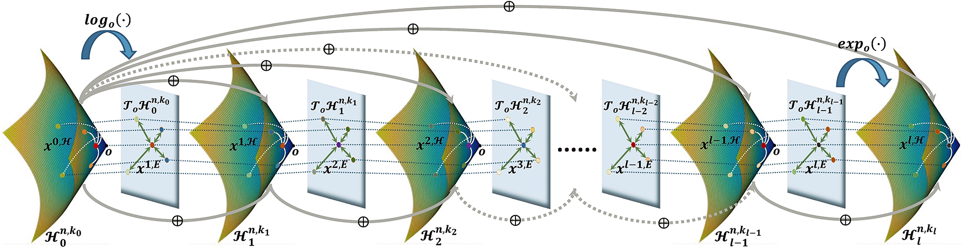
Figure 1: The overall architecture of hyperbolic deep graph convolutional neural network (HDGCNN)

As depicted in Fig. 1, we designate the origin o as the reference point for the hyperbolic space. We initiate the embedding of the initial node located in the hyperbolic space ℋ0n,k0 as x0,ℋ and then project it onto the tangent space ℐoℋ0n,k0 through the logarithmic mapping logo(⋅). Subsequently, a graph convolution operation is executed in ℐoℋ0n,k0 to aggregate neighborhood information and yield x1,E. This newly obtained node embedding x1,E is then projected into the subsequent hyperbolic space ℋ1n,k1 using the exponential mapping expo(⋅), resulting in x1,ℋ. The above operations are repeated iteratively until the final output xl,ℋ is achieved. Furthermore, HDGCNN employs a dense connection architecture to link the output of each layer of the hyperbolic space with the initial node embedding, thereby effectively encoding high-order neighborhood information.

4.1 Hyperbolic Initialization Layer of HDGCNN

As an end-to-end graph representation learning framework, HDGCNN is designed to directly process raw graph data as input. However, since the original input graph is defined in the Euclidean space, we aim to enhance feature representation and alleviate graph embedding distortion by embedding the scale-free or hierarchical graph into the hyperbolic space. To achieve this, the node features in the Euclidean space are initially mapped into the hyperbolic space through the inception layer of HDGCNN.

Let G=(V,ع) denote the input graph, and (xi0,E)i∈V∈Rn represent the input Euclidean node features. We establish the origin o:={k,0, …, 0}∈ℋn,k as a reference point for the hyperbolic space ℋn,k, which possesses a constant negative curvature of −1/k. This choice of origin facilitates the embedding of nodes from the hyperbolic space into the projection into the tangent space ℐoℋn,k.

Fig. 2 shows how to project the initial input node (xi0,E)i∈V of the Euclidean space onto the hyperboloid manifold ℋ0n,k. Here, the subscript l of ℋln,k denotes the l-th layer hyperbolic manifold. Utilizing the exponential mapping function expok(⋅) from Eq. (6), we can project xℐo=(0,x0,E) to ℋ0n,k. In this context, o represents the origin of ℋ0n,k, and (0,xE) can be represented as a point in the tangent space ℐoℋn,k, satisfying ⟨(0,xE), o⟩=0. In the initial layer, we denote the initial input nodes as (0,x0,E), and (0,x0,E) is mapped by expok(⋅) to obtain (xi0,ℋ)i∈V. To summarize, through the initial layer of HDGCNN, the initial node embeddings in Euclidean space are mapped to the first layer of hyperbolic manifold embeddings, as shown in Eq. (8):

x0,ℋ=expok((0,x0,E))(8)

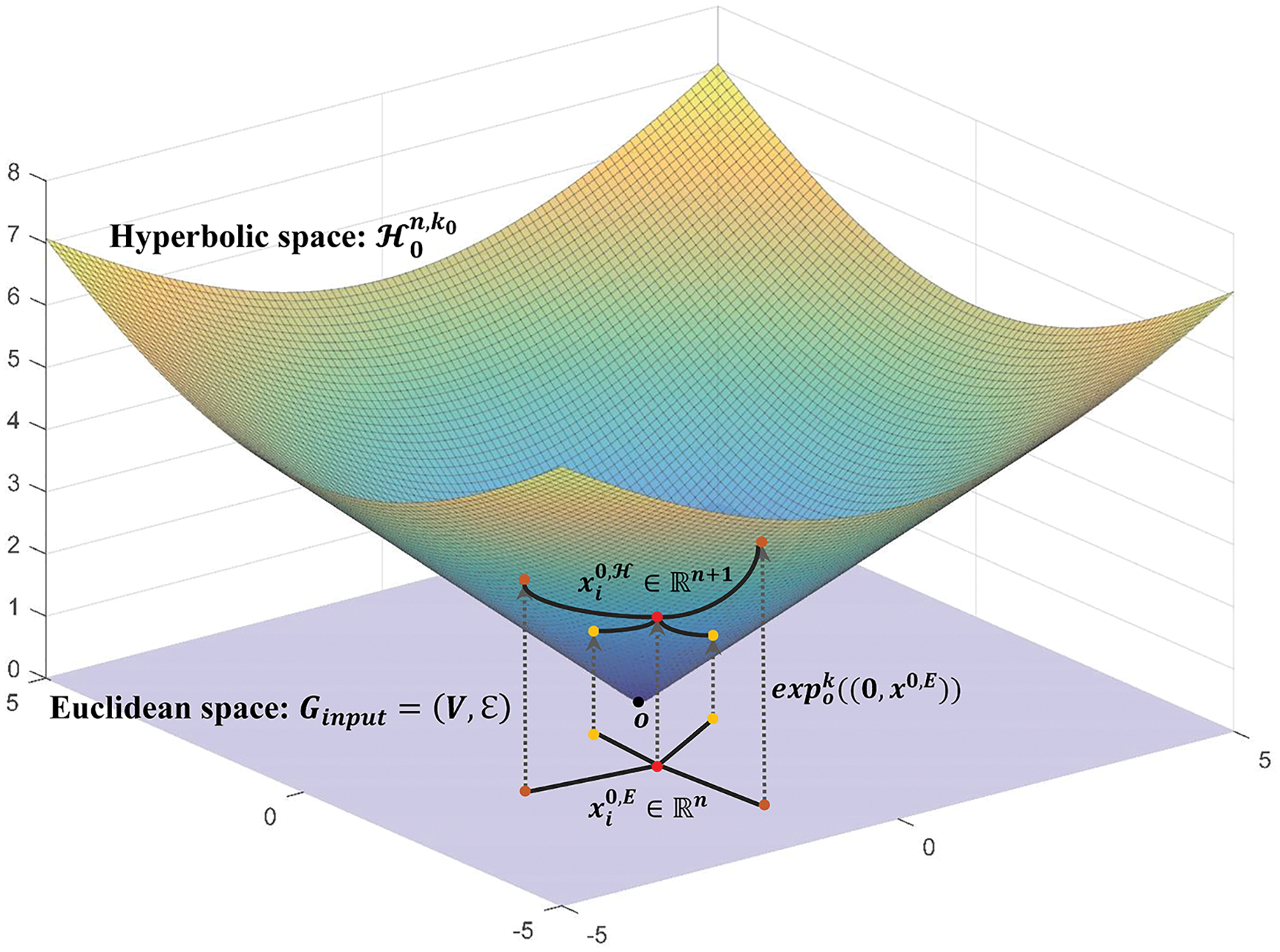
Figure 2: Projection of input nodes from euclidean space to hyperboloid manifold

4.2 Feature Transformation Based on Identity Mapping in Hyperbolic Space

Feature transformation plays a pivotal role in the graph convolution operation, serving as a crucial data enhancement technique to elevate low-dimensional node embeddings into a higher-dimensional space. By capturing inter-feature relationships, feature transformation enables the learning of more refined node features, thereby significantly enhancing graph representation learning performance. Moreover, for datasets with excessively high node feature dimensions, feature transformation can effectively reduce the computational complexity and improve overall efficiency.

The essence of feature transformation lies in mapping the node embeddings from the previous layer to the embedding space of the subsequent layer. Let Xl,E∈R|V|×nl and Xl−1,E∈R|V|×nl−1 denote the node feature matrices of the l-th and l−1-th layers of the GCN in the Euclidean space, respectively. Additionally, let W∈Rnl−1×nl be a learnable weight matrix. The feature transformation adopted by GCN can be formulated as Eq. (9):

Xl,E=Xl−1,EWl(9)

In our endeavor to conduct feature transformation operations on Xℋ∈ℋn,k within hyperbolic space, we encounter a challenge due to the absence of a vector space structure in this setting. Consequently, it becomes necessary to execute feature transformations in the tangent space ℐoℋn,k, which is situated at the reference point o within the hyperbolic space.

4.2.1 Feature Transformation Based on Identity Mapping in GCNs

To exploit remote dependencies and non-local structural features among nodes, our objective is to develop a deep graph convolution network model. The iterative aggregation and update operations of the graph convolution layer facilitate the extraction of more refined non-local node features. However, a concern arises from the work of Klicpera et al. [51], who identified that frequent interactions between feature matrices of different dimensions can lead to performance degradation in the model. To address this issue, Chen et al. [26] drew inspiration from the concept of identity mapping in ResNet and propose the incorporation of both unit and weight matrices with varying weights. Specifically, as the number of layers deepens, the weight of the unit matrix increases while the weight value of the weight matrix diminishes. This feature transformation approach using identity mapping is expressed as follows, denoted by Eq. (10):

Xl,E=Xl−1,E((1−δl)In+δlWl)(10)

δl=(λl+1.8)(11)

In the Eq. (10), In denotes the identity matrix, while δl represents the weight decay parameter, which adapts dynamically with the layer index l. As the number of layers deepens, the value of δl gradually decreases. Additionally, λ in Eq. (11) is a manually set hyperparameter, controlling the decay rate of δl. This design guarantees that the deep model can achieve performance at least on par with that of the shallow model.

4.2.2 Hyperbolic Feature Transformation Based on Identity Mapping

To perform feature transformation in the hyperbolic space ℋn,k, a two-step process is employed. Firstly, nodes in the hyperbolic space are projected to the tangent space ℐoℋn,k near the hyperbolic reference point using the logarithmic mapping function logok(⋅) from Eq. (7). Subsequently, feature transformation based on the identity mapping is carried out in the tangent space, and the resulting node features are then mapped back to the hyperbolic space using the exponential map expok(⋅) from Eq. (6).

Let Xl,ℋ∈R|V|×n and Wl∈Rn×n′ respectively represent the node feature matrix and weight matrix in the l-th layer of the hyperbolic space. We define the matrix multiplication in the hyperbolic space based on identity mapping as Eq. (12):

Xl,ℋ⊗kWl:=expok(logok(Xl,ℋ)((1−δl)In+δlWl))(12)

The functions logok:ℋk→ℐoℋk and expok:ℐoℋk→ℋk represent the logarithmic mapping and exponential mapping, respectively. The aforementioned Eq. (12) facilitates the hyperbolic transformation of Xl,ℋ∈R|V|×n to Xl,ℋ∈R|V|×n′. It is important to elucidate the significance of introducing identity mapping mechanisms in hyperbolic transformations. As pointed out by He et al. [52], the benefits of feature transformation in the graph convolution process are minimal. However, we aim to employ the feature transformation mechanism to enhance the model’s flexibility. Consequently, with our proposed hyperbolic transformation method, HDGCNN evolves towards direct neighborhood information aggregation as the number of layers deepens. This approach reduces model overfitting and accelerates training and inference processes.

4.3 Neighborhood Aggregation on Hyperbolic Manifolds

Neighborhood aggregation plays a crucial role in GCNs. It involves updating a node embedding xi by aggregating information from its first-order neighbors (xj)j∈N(i). In deep models, iterative graph convolution layers enable the aggregation of high-order neighborhood information to capture global features. For hyperbolic neighborhood aggregation, the first step is to calculate the neighborhood weight coefficients. These weights can be computed using various methods, such as structural information [13,53], node distance [54], or feature attention [55]. Next, we can aggregate neighborhood information using the computed neighborhood weight coefficients. However, these coefficients are calculated based on node features and reflect the importance between different nodes. As the number of layers increases, learned node features gradually stabilize. Continuing to use node features for calculating the weight coefficients may lead to overfitting. Therefore, we aim to primarily employ neighborhood weight coefficients for neighborhood aggregation in the shallow part of HDGCNN, and rely on the graph’s structural features for aggregation in the deeper layers. This way, HDGCNN can effectively utilize both structural and node feature information, adapting to deep model architectures. As for dynamically allocating the weight coefficients for structural and node features for neighborhood information aggregation, we will adaptively learn based on the model’s layer changes. Further details on this approach can be found in the subsequent sections.

4.3.1 Computation of Attention Coefficient between Nodes on Hyperbolic Manifold

In our approach, we update the inter-node attention coefficients based on the hyperbolic node features learned in each layer of HDGCNN. This enables us to aggregate neighbor information considering both the structural information and the significance of the first-order neighbor nodes with respect to the central node. Our attention coefficient calculation method is inspired by the Graph Attention Network (GAT) proposed by Veličković et al. [56]. However, the original GAT calculates attention coefficients based on node features in the Euclidean space. In our work, we extend this method to hyperbolic manifolds. Given the hyperbolic embeddings of two nodes at layer l, denoted as (xil,ℋ, xjl,ℋ), we utilize the following Eq. (13) to compute attention weights between nodes:

(AGATl)ij=exp(LeakyReLU((al)T[Wllogok(xil,ℋ)∥Wllogok(xjl,ℋ)]))∑u∈Niexp(LeakyReLU((al)T[Wllogok(xil,ℋ)∥Wllogok(xul,ℋ)]))(13)

Among them, logok(⋅) maps points from the hyperbolic manifold to the tangent space at the origin, “||” represents the concatenation operation, and the superscript T denotes the transpose operation. The embedding representation logok(xl,ℋ)∈Rn on the Euclidean plane undergoes a linear transformation using the weight matrix Wl∈Rn′×n, followed by a concatenation operation to obtain the concatenated vector (Wllogok(x⋅l,ℋ)∥Wllogok(x⋅l,ℋ))∈R2n′. The weight vector al∈R2n′ is then applied to project the concatenated vector onto a scalar. It is important to note that, for the adjacency matrix, if the edge does not exist between two nodes, the corresponding element in AGAT is set to 0, ensuring that the edge information is appropriately handled.

4.3.2 Neighborhood Aggregation Based on Structural Features and Hyperbolic Attention Coefficient

To fully leverage structural information and node features for neighborhood aggregation, we propose a method based on initial structural features and hyperbolic attention coefficients, and construct an adjacency matrix using skip connections. Specifically, the adjacency matrix used in the l-th layer of HDGCNN is composed of the initial adjacency matrix Aadj∈RN×N and the AGATl∈RN×N matrix.

The initial adjacency matrix Aadj contains the structural information of the input graph G=(V,ع). Each element of Aadj is either 1 or 0, indicating the presence or absence of an edge at the corresponding position, respectively. It is defined as Eq. (14):

(Aadj)ij={1, eij∈E 0, eij∉E (14)

In order to incorporate both structural information and inter-node attention coefficients during the process of aggregating neighborhood information, we propose the following method to calculate the adjacency matrix, as shown in Eq. (15).

Al=(1−δl)Aadj+δlAGATl(15)

The parameter δl in Eq. (15) represents the weight decay parameter that adapts with the number of layers l. As the number of layers deepens, δl gradually decreases. The value of δl follows the same formulation as in Eq. (11), where λ is a hyperparameter. We adopt this approach because the node features learned by the shallow model may not be as refined, so we assign more weight to the adjacency matrix AGAT, which contains node feature information, to facilitate its updates during backpropagation. Conversely, as the number of layers increases, the learned node features tend to stabilize. We aim to capture long-range dependencies and non-local structural features between nodes through the iterations of the deep model. Thus, we assign more weight to the adjacency matrix Aadj, which contains structural information, while reducing the weight of AGAT. The adjacency matrix construction method using skip connections is illustrated in Fig. 3.

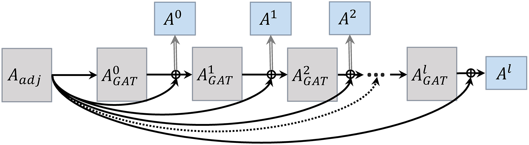
Figure 3: The adjacency matrix A is constructed using Aadj and AGAT with skip connections

4.3.3 Hyperbolic Neighborhood Aggregation

In order to effectively compute neighborhood aggregation weights by leveraging both structural information and feature attention, we introduce the adjacency matrix construction method with skip connections as described earlier. In the shallow layers, the aggregation of first-order neighbor information by central nodes is primarily influenced by the attention coefficient in AGAT. As the model goes deeper, the aggregation of neighborhood information by central nodes is predominantly influenced by the adjacency matrix Aadj, which represents the structural information. AGAT and Aadj dynamically adjust their respective weight values according to the changes in the number of layers, ultimately forming an integrated adjacency matrix A. Consequently, our proposed neighborhood aggregation method on hyperbolic manifolds can be summarized as Eq. (16):

AGGk(xℋ)i=expok(∑j∈N(i)Aijlogok(xjℋ))(16)

4.4 Non-Linear Activation

The nonlinear activation method is performed as Eq. (17). Initially, the node embeddings on the hyperbolic manifold ℋn,kl−1 with curvature −1/kl−1 are mapped to the tangent plane ℐoℋn,kl−1 at the origin o using logokl−1(⋅). Then, a nonlinear activation σ(⋅) is applied in the Euclidean space to the mapped embeddings. Finally, expokl(⋅) is used to map the results after nonlinear activation back to the hyperbolic manifold ℋn,kl:

σ⊗kl−1, kl(xℋ)=expokl(σ(logokl−1(xℋ)))(17)

Since our HDGCNN adopts learnable curvature, each layer of the hyperbolic manifold has a different curvature, and non-linear activation enables the curvature to be updated across layers. Hence hyperbolic nonlinear activations σ⊗kl−1, kl(⋅) [55] with different curvatures are introduced.

4.5 Dense Connections Based on Non-Local Message Passing Framework

To construct a hyperbolic deep graph convolutional neural network (HDGCNN) model that can effectively capture remote dependencies between nodes in scale-free graphs or hierarchical graphs with power-law distributions, as well as finer node features, and address the over-smoothing issue caused by deep models, we draw inspiration from the design principles of ResNet and DenseNet [57]. We adopt the concept of skip connections to propagate the initial node features x0,ℋ embedded in the hyperbolic space from the initial layer of HDGCNN to the output of each subsequent layer, and further pass the output of each layer to the subsequent layers. This non-local message passing framework enables us to effectively build hyperbolic deep graph convolutional neural network models, as shown in Eqs. (18) and (19):

zil,ℋ=∑j∈N(i)Ml(xil−1,ℋ,xjl−1,ℋ)(18)

xil,ℋ=Ul(zil,ℋ,xil−1,ℋ,xi0,ℋ)(19)

In the above Eq. (18), Ml represents the message function of the l-th layer. It aggregates the features of node i and its first-order neighbors in the hyperbolic space of the l−1-th layer, obtaining the hyperbolic node features zil,ℋ after neighbor information aggregation in hyperbolic space. Ul in Eq. (19) denotes the update function of the l-th layer. Leveraging dense connections, it adaptively accumulates and updates the initial node features, the output results of the previous layer, and the results of the hyperbolic graph convolution of this layer, ultimately obtaining the hyperbolic embedding of node i in the l-th layer. The specific update method is defined as shown in Eq. (20):

Ul(zil,ℋ,xil−1,ℋ,xi0,ℋ)=α1lzil,ℋ+α2lxil−1,ℋ+α3lxi0,ℋ(20)

Among them, α1l, α2l, and α3l are learnable weight coefficients, and the model automatically learns these weight coefficients during the backpropagation process to aggregate the values of zil,ℋ, xil−1,ℋ, and xi0,ℋ, respectively. Through this densely connected design, HDGCNN achieves feature reuse, ensuring that it attains at least the same level of performance as shallow models. Additionally, the deep network structure facilitates the non-local information aggregation of nodes, leading to the extraction of more refined node features.

4.6 Architecture of HDGCNN

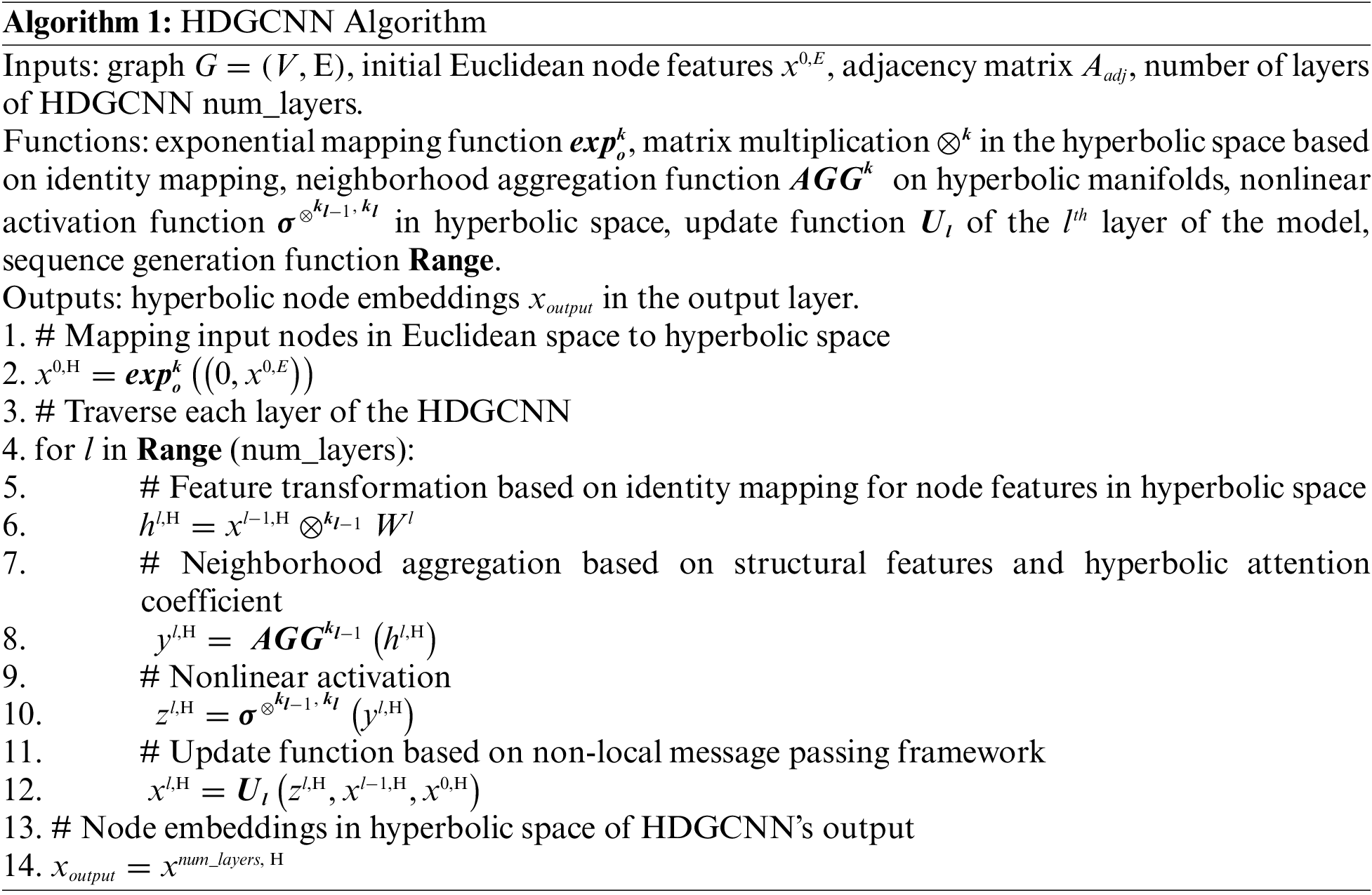
This section provides a comprehensive summary of all the modules employed in HDGCNN as mentioned earlier. Given an input graph G=(V,ع), where the input Euclidean features are denoted as (xi0,E)i∈V. Firstly, the hyperbolic input features, (xi0,ℋ)i∈V, are obtained by mapping the Euclidean features to the hyperbolic space through the initial layer, as explained in Section 4.1. These hyperbolic input features then undergo a hyperbolic transformation based on identity mapping, utilizing Eq. (21), as explained in Section 4.2.

Next, neighborhood aggregation is performed on nodes using structural features and hyperbolic attention coefficients, achieved by Eq. (22), as explained in Section 4.3. Subsequently, a nonlinear activation is applied to the neighborhood aggregation results using a learnable curvature, as presented in Eq. (23), as explained in Section 4.4. Finally, Eq. (24) is employed to create dense connections among the output results of each HDGCNN layer based on the novel non-local message passing framework, facilitating the capture of more refined high-order features of nodes, as elucidated in Section 4.5.

The aforementioned four steps constitute a hyperbolic graph convolutional layer, and HDGCNN is formed by stacking multiple hyperbolic graph convolutional layers. The algorithm description of the HDGCNN is shown in Algorithm 1.

hil,ℋ=xil−1,ℋ⊗kl−1Wl(21)

yil,ℋ=AGGkl−1(hl,ℋ)i(22)

zil,ℋ=σ⊗kl−1, kl(yil,ℋ)(23)

xil,ℋ=Ul(zil,ℋ,xil−1,ℋ,xi0,ℋ)(24)

5  Experiments

In this section, we present an extensive series of experiments to thoroughly evaluate the performance of HDGCNN on both node classification and link prediction tasks. The main objective is to showcase the effectiveness and capabilities of HDGCNN in addressing these crucial graph-related tasks. To achieve this, we conduct a comparative analysis by benchmarking HDGCNN against shallow methods, neural network-based methods, GNN-based methods, hyperbolic GNN-based methods, and other state-of-the-art approaches. Moreover, we perform ablation experiments to assess the impact and effectiveness of our proposed building blocks. Through these rigorous and diverse experiments, we aim to establish the superiority of HDGCNN over existing methods. The results of these experiments will underscore the potential and significance of HDGCNN as a powerful tool for graph representation learning.

5.1 Experiment Setup

5.1.1 Datasets

The HDGCNN proposed in this paper is specifically designed to handle scale-free or hierarchical graphs with tree structures, enabling the embedding of such graphs into hyperbolic spaces with reduced distortion. To assess the effectiveness of HDGCNN in handling tree-structured graphs, we carefully selected four datasets with varying degrees of tree-like characteristics. The details of these datasets are summarized in Table 1 for reference and comparison purposes. By conducting experiments on these datasets, we aim to demonstrate how HDGCNN performs in capturing and preserving the tree structures, and how it outperforms other methods in terms of node classification and link prediction tasks.

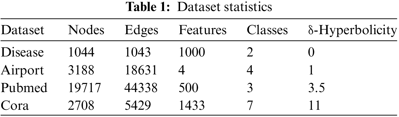
We evaluate the tree-like characteristics of the datasets using Gromov’s δ-Hyperbolicity [58]. A smaller value of δ-Hyperbolicity indicates a higher degree of treeness in the dataset. For our experiments, we carefully selected four datasets with varying δ values, namely Disease, Airport, Pubmed, and Cora, to thoroughly assess the effectiveness of our proposed method. The Disease dataset represents a disease propagation tree, simulating the SIR disease transmission model [59], with each node representing either an infection or a non-infection state. The Airport dataset consists of airports and routes, where nodes represent airports, and edges represent routes between them. Pubmed and Cora [60] are citation datasets, where nodes represent scientific papers, edges represent citation relationships, and the node labels correspond to the academic fields of the papers.

5.1.2 Baselines

To comprehensively evaluate the performance of HDGCNN, we compare it against a variety of state-of-the-art methods, which can be categorized as follows: shallow methods, neural network-based methods (NN), graph neural network-based methods (GNN), and hyperbolic graph neural network-based methods. The shallow methods we consider are Euclidean-based embedding (EUC) and Poincare sphere-based embedding (HYP) [35]. As for the NN methods, we include feature-based MLP and its hyperbolic variant (HNN) [34]. For the GNN category, we select GCN [13], GAT [56], SAGE [14], and SGC [61], as these methods have demonstrated exceptional performance in various applications by fully leveraging node features and structural characteristics. Additionally, we evaluate hyperbolic GNN methods, including HGCN [55], HGNN [53], HGAT [62], and HGCF [63], which represent hyperbolic versions of the GNN approaches mentioned earlier. By comparing HDGCNN with these state-of-the-art methods, we can thoroughly assess its performance and demonstrate its advantages in various scenarios.

5.1.3 Parameter Settings

For the sake of fairness, we adopt consistent dataset splits for all baseline methods and models. In the node classification (NC) task, we employ a 30/10/60% split for Disease, and a 70/15/15% split for Airport, which are designated for training, validation, and testing, respectively. As for the Pubmed and Cora datasets, we follow the same split strategy as proposed by Yang et al. [64]. In the link prediction task, the edges in all datasets are randomly distributed with a ratio of 85/5/10%. Across all datasets, we set the learning rate to 0.01, dropout to 0, weight decay parameter to 0, bias parameter to 1, and λ in Eq. (11) to 0.9. We configure the curvature to self-learn mode and employ the Adam optimizer [65] for model optimization. The maximum number of training epochs is set to 5000, with early stopping based on a window size of 100 epochs, where training stops if the validation loss does not decrease continuously for 100 epochs. The minimum number of training epochs is set to 100. We employ ReLU activation as the linear activation for hidden layers. The LeakyReLU activation function is used as the linear activation function in the hyperbolic attention coefficient module, with its negative slope set to 0.2. For numerical stability in optimization, we choose the Lorentz (Hyperboloid) model as the Riemannian manifold. The parameters r and t for the Fermi-Dirac decoder used in the link prediction task are set to 2 and 1, respectively.

To ensure a fair comparison between HDGCNN and the hyperbolic GNN baseline method, we represent node features using a 16-dimensional representation. In this paper, we deploy a 32-layer HDGCNN model, while the hyperbolic GNN baseline method adopts a 4-layer model structure. These choices are made to provide a comprehensive assessment of the performance of HDGCNN in comparison with the hyperbolic GNN baseline method. The detailed model configurations and parameter settings can be accessed at the following link: https://github.com/FrancisJUnderwood/hdgcnn/tree/master.

5.2 Results

We present the performance comparison of HDGCNN with other baseline methods in Table 2. For the link prediction task, we employ the area under the ROC curve (AUC) on the test set as the evaluation metric. For the node classification task, we use the F1 score to assess the performance of node classification.

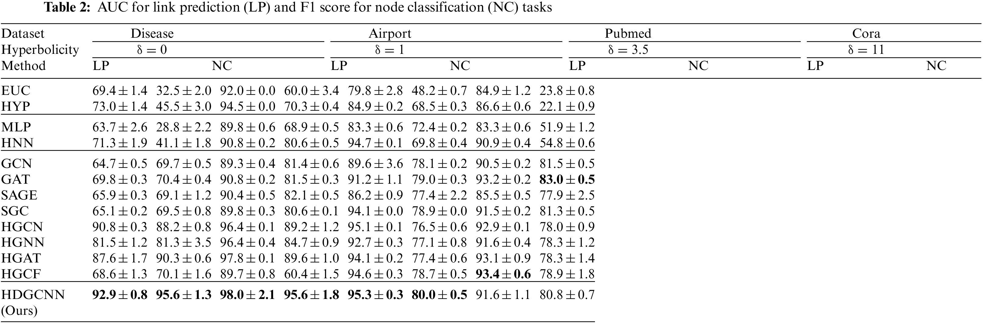
Analyzing the results in Table 2, we observe that HDGCNN outperforms a considerable number of baseline methods on datasets with evident tree structures (low δ values). In the Disease dataset with δ = 0, HDGCNN achieves an average accuracy approximately 26.5% higher in link prediction (LP) and 24.8% higher in node classification (NC) compared to the Euclidean-based GNN baseline method. Moreover, HDGCNN shows an average of about 10.8% higher accuracy in LP and 17.5% higher accuracy in NC than the hyperbolic GNN baseline method. HDGCNN also demonstrates competitive performance on the Airport and Pubmed datasets.

However, on the Cora dataset where the tree structure is less apparent (high δ value), the Euclidean-based GNN methods HGCF and GAT attain the best results in link prediction and node classification tasks, respectively. Despite this, HDGCNN still achieves notable performance on the Cora dataset, showcasing its versatility and potential in various graph-related tasks.

5.2.1 Analysis

We Analysis reveals the following key insights:

(1) By comparing the experimental results of HDGCNN with those of the Euclidean-based GNN method, we discern that graph data exhibiting a tree structure can indeed benefit from hyperbolic geometry. The experimental findings across the Disease, Airport, and Pubmed datasets substantiate this assertion. Notably, HDGCNN shines remarkably on the Disease dataset, which exhibits the highest degree of tree-like structure (δ = 0), showcasing a substantial performance advantage over the Euclidean-based GNN baseline method. As the tree-like structure weakens (δ value increases), HDGCNN maintains its significant performance lead over the GNN baseline method on the Airport and Pubmed datasets, albeit with a diminished margin compared to the Disease dataset.

(2) A comparative analysis between HDGCNN and hyperbolic GNN methods illustrates that hyperbolic GNN methods can indeed benefit from a deep model structure. This deduction is corroborated by results across the four datasets and is further validated in the subsequent node embedding visualization analysis in Section 5.4.3. Empirical findings demonstrate that HDGCNN, with its deep model architecture, surpasses all shallow hyperbolic GNN baseline methods in link prediction and node classification tasks. It is notable that HGCF and GAT achieve optimal outcomes in link prediction tasks and node classification on Cora datasets, respectively. Our analysis posits that this could be attributed to the fact that HGCF employs fewer operations on hyperbolic maps and extensively utilizes graph convolution operations within the Euclidean tangent space. Additionally, given the Cora dataset’s diminished tree-like nature, it tends to benefit more from Euclidean geometry.

(3) Furthermore, it is worth noting that MLP and its hyperbolic variant, HNN, are feature-based methods that do not leverage graph structural information and lack an information aggregation step. The discernible performance disparity observed between MLP, HNN, and HDGCNN, along with other hyperbolic GNN baseline methods, in the context of node classification tasks, demonstrates the significance and efficacy of neighborhood information aggregation in learning node feature representations. This observation reinforces the conclusions drawn by Chami et al. [55].

Collectively, these findings underscore the efficacy and versatility of HDGCNN across various graph-related tasks, reaffirming its position as a promising approach in graph representation learning.

5.3 Ablation Experiment

In this section, we conduct a series of ablation experiments aimed at systematically validating the indispensability of each proposed component within HDGCNN. We meticulously assess the contributions of the identity mapping-based feature transformation module, the neighborhood aggregation module, and the non-local message passing framework, individually. To achieve this, we progressively exclude these modules from HDGCNN and evaluate the resulting model performance. The derived variant models, denoted as HDGCNN-Trans, HDGCNN-Agg, and HDGCNN-NoneLocal, correspondingly represent models in which the feature transformation method, neighborhood aggregation method, and non-local message passing framework have been substituted. In more detail, HDGCNN-Tran substitutes the feature transformation method with a conventional linear transformation [53,55,63], while HDGCNN-Agg employs a conventional weighted aggregation [13] as a replacement for the neighborhood aggregation method. The performance of HDGCNN and the three variant models across node classification tasks on the four datasets is comprehensively summarized in Table 3.

5.3.1 Analysis

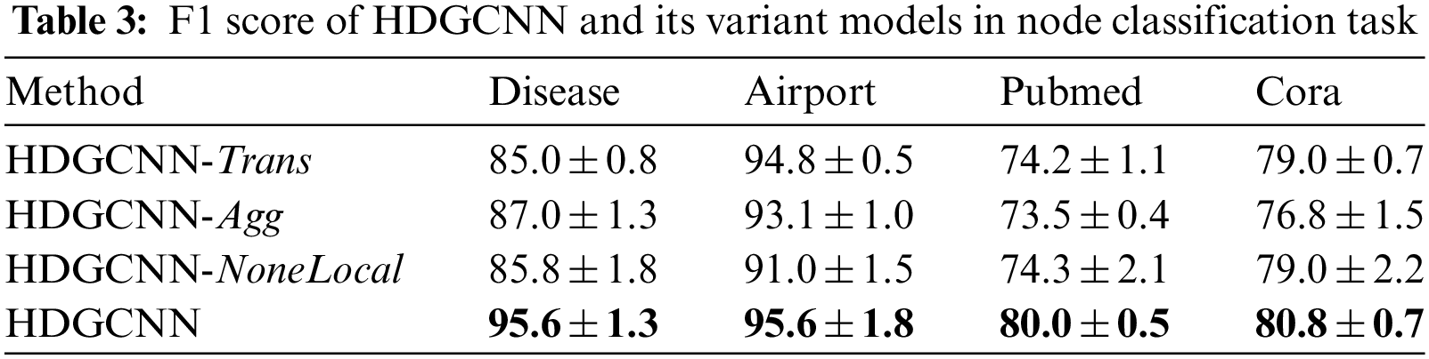
The analysis of the results presented in Table 3 reveals a consistent trend of decreased model performance upon the removal of each individual component. Notably, on datasets such as Disease and Airport, characterized by a pronounced treeness degree, the non-local message passing framework emerges as a pivotal element. The absence of this module leads to a conspicuous decline in HDGCNN’s performance. Similarly, on the Pubmed dataset, the omission of any module leads to a substantial reduction in performance. In the case of the Cora dataset, the removal of our proposed neighborhood aggregation module results in a significant performance degradation.

These observations provide further substantiation of our findings in Section 5.2.1, indicating that datasets characterized by a lower tree structure degree are more likely to benefit from Euclidean geometry. Moreover, these results underscore the essential role of neighborhood information aggregation in the effective acquisition of node feature representations. Concurrently, they affirm the superior performance of our proposed neighborhood aggregation approach in contrast to conventional methods.

5.4 Quantitative and Qualitative Analysis of Over-Smoothing

In this section, we will conduct a quantitative analysis of HDGCNN’s capacity to alleviate over-smoothing, while also undertaking a qualitative assessment of its aptitude in capturing distant high-order node features through node embedding visualization. Initially, we introduce a smoothness evaluation metric to quantify the smoothness of each layer’s output in the model—smoothness, in this context, refers to the similarity among nodes within the graph. By comparing the smoothness across various layers of three hyperbolic graph neural network models—namely HDGCNN, HGCN, and HGCF—we substantiate HDGCNN’s suitability for constructing hyperbolic deep graph neural network architectures. These architectures excel in extracting refined node features from graph data characterized by tree-like structures, thereby mitigating issues related to over-smoothing. Subsequently, we proceed to visualize the node embeddings generated by the aforementioned hyperbolic graph neural network models. By discerning clustering patterns among different categories of nodes in the visualization space, we qualitatively underscore HDGCNN’s proficiency in capturing intricate node features.

5.4.1 Evaluation Metric of Smoothness

The over-smoothing problem caused by deep graph neural network models originates from the fact that each node in the graph aggregates information from almost the entire graph due to the multi-layer graph convolution operation. This ultimately leads to the convergence of all node features, resulting in closely embedded nodes spatially. To address this, we employ the Mean Average Distance (MAD), as proposed by Chen et al. [66], as a quantitative measure. MAD assesses smoothness by calculating the average distance between nodes. Smoothness is utilized to represent the similarity of node embeddings: a larger MAD value signifies lower embedding similarity, while a smaller MAD value indicates higher similarity. The calculation method for the MAD value is presented in Eqs. (25) to (28).

MADtgt=∑i=0nD¯itgt∑i=0n1(D¯itgt)(25)

D¯itgt=∑j=0nDijtgt∑j=0n1(Dijtgt)(26)

Dtgt=D∘Mtgt(27)

Dij=1−xiℋ⋅xjℋ|xiℋ|⋅|xjℋ| i,j∈[1,2,…,n](28)

Eq. (25) delineates the procedure for computing the MAD value of a given pair of target nodes, where 1(x) equals 1 if x > 0, and 0 otherwise. Eq. (26) is utilized to determine the average of non-zero elements within each row of matrix Dtgt. Within Eq. (27), Mtgt symbolizes an N×N mask matrix, while ○ denotes the element-wise multiplication operation that filters information from the N×N distance matrix D using the mask matrix Mtgt. The calculation of the distance matrix D is presented in Eq. (28). Here, xiℋ and xjℋ denote the hyperbolic feature vectors of nodes i and j, respectively, and the distance matrix D is computed by evaluating the cosine values between all pairs of nodes. It is important to highlight that the node feature matrix xℋ represents the hyperbolic output from the final layer of HDGCNN.

5.4.2 Quantitative Analysis of Over-Smoothing

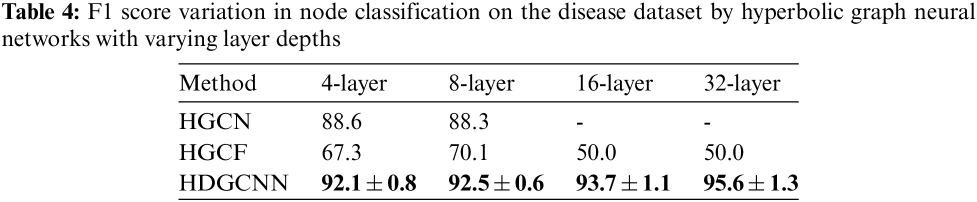
Ordinary GCN models typically exhibit a shallow architecture comprising 3 to 4 layers. To enhance the depth of the graph convolutional network and effectively capture non-local structural features and long-range interdependencies among nodes, we seek to extend the network’s depth. However, deeper networks often encounter the challenge of excessive smoothing. To address this concern, we present HDGCNN, a solution that facilitates the creation of deep network architectures without succumbing to the issue of excessive smoothing, thereby enhancing node feature extraction.

In Table 4, we present the F1 scores of three hyperbolic graph neural network models—namely, HGCN, HGCF, and HDGCNN—across varying layer model structures during node classification tasks on the Disease dataset. Our observations reveal that HGCN fails to yield performance improvements upon increasing the number of network layers. Notably, as the network depth reaches 16 layers, the model encounters a gradient disappearance issue, rendering it untrainable. Similarly, while HGCF’s performance deteriorates significantly with deeper network architectures, HDGCNN’s performance remains stable and even exhibits improvement. These findings underscore that hyperbolic graph neural networks are susceptible to over-smoothing, a challenge effectively addressed by HDGCNN.

Subsequently, we embark on a quantitative analysis of the smoothness exhibited by distinct hyperbolic neural network models across varying depths. Depicted in Fig. 4 are the Mean Average Distance (MAD) values of three models–HGCN, HGCF, and HDGCNN–across different layers while performing node classification tasks on the Disease dataset. Lighter colors indicate smaller MAD values, signifying more pronounced node over-smoothing. The outcomes observed in the analysis indicate a pivotal trend. Specifically, as the depth of HGCN reaches 16 layers, the MAD value converges to 0, indicating that the nodes in the graph have become indistinguishable. Notably, the MAD value of HGCF progressively diminishes with increasing network depth, with a particularly substantial decline by the time the depth reaches 16 layers. Conversely, HDGCNN’s MAD value remains consistently within a stable range as the network depth increases, exhibiting even a propensity to rise. This conspicuous trend reaffirms the efficacy of our proposed HDGCNN in seamlessly amalgamating a deep graph neural network architecture with hyperbolic geometry. More remarkably, it adeptly circumvents the over-smoothing conundrum characteristic of hyperbolic graph neural networks.

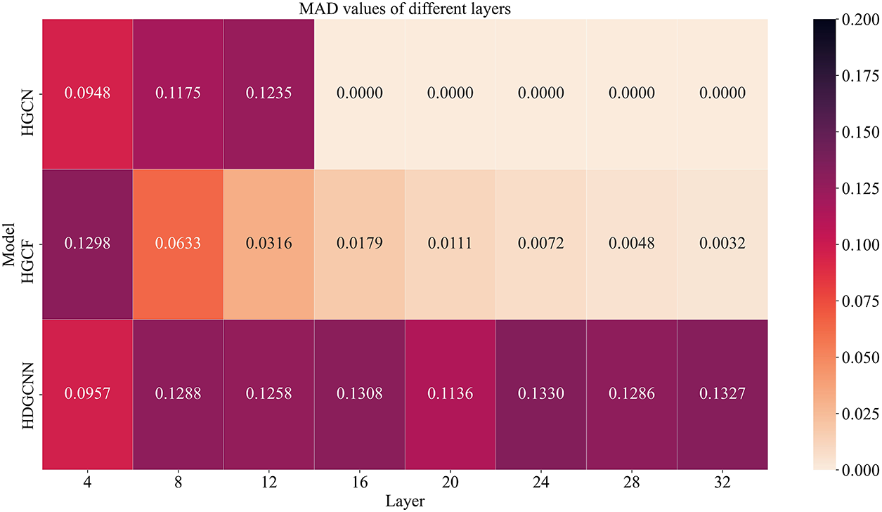
Figure 4: MAD values for HGCN, HGCF, and HDGCNN across layers in the disease dataset

5.4.3 Node Embedding Visualization

In order to visualize the node classification results, we project the node embeddings generated by the three hyperbolic graph neural network models into a 3-dimensional space. As depicted in Fig. 5, each row illustrates the visualization outcomes of node embeddings produced by HGCN, HGCF, and HDGCNN across the four datasets. Correspondingly, each column corresponds to the node embeddings of the Disease, Airport, Pubmed, and Cora datasets from left to right.

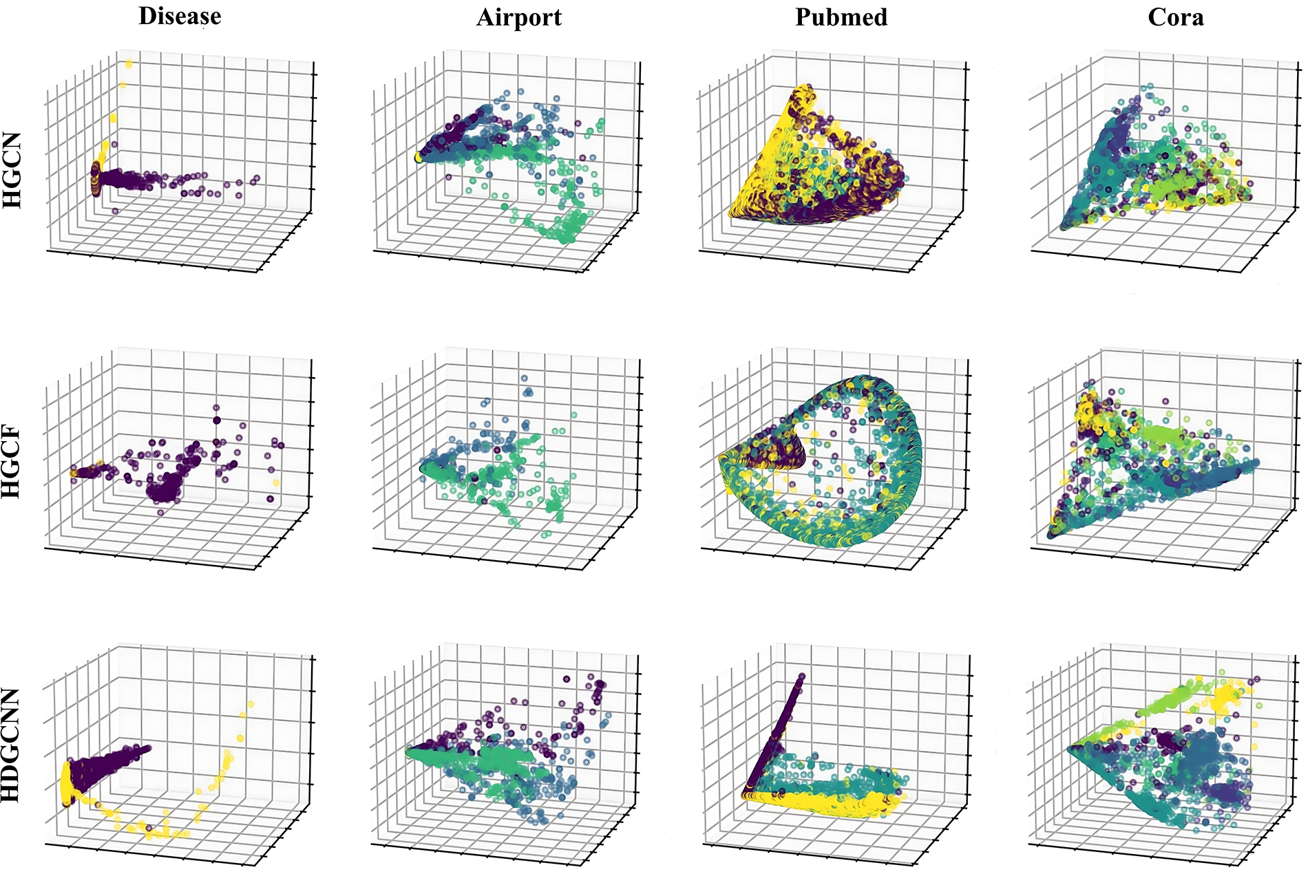
Figure 5: Visualization of node embeddings

The visualization in the Fig. 5 reveals that HDGCNN consistently attains superior classification performance on all datasets. Within the hyperbolic space, nodes of each class exhibit distinct clustering, with minimal confusion in node embedding representations. It is noteworthy that nodes closer to the hyperboloid’s origin generally occupy higher hierarchy levels within the tree structure. These outcomes underscore HDGCNN’s capability to seamlessly transform Euclidean-based node embeddings into hyperbolic embeddings, effectively preserving the hierarchical structure.

By comparing HDGCNN with HGCN and HGCF, we further confirm that deep model structures confer an advantage to hyperbolic graph neural networks.

5.5 Attention Distribution and Parameter Sensitivity Analysis

5.5.1 Attention Distribution

In this section, we will delve into an analysis of the attention coefficients acquired by three models: HGCN, HGCF, and HDGCNN. The aim is to ascertain whether HDGCNN effectively employs the hyperbolic neighborhood aggregation method, grounded in structural features and hyperbolic attention coefficients, to learn attention weights. To initiate this examination, we introduce a disparity metric on the attention coefficient matrix A pertaining to node i, denoted as Δi=A[i,:]−Uidegree(vi) [67], where Ui signifies the uniform distribution score of node i. The metric Δi serves to gauge the degree of deviation between the acquired attention coefficient and the uninformative uniform distribution. Notably, a larger Δi value indicates a more meaningful learned attention coefficient. By contrasting the discrepancy metric distributions across the attention coefficient matrix (as given by Eq. (15)) obtained from HDGCNN’s output layer with those yielded by HGCN and HGCF, we present the specific outcomes in Fig. 6a. Illustrated in Fig. 6a are the disparity metric distributions of attention matrices learned by the aforementioned models on the Airport dataset. The figure distinctly reveals that the attention coefficients learned by HDGCNN exhibit larger variance. Conversely, the attention coefficients acquired by HGCN and HGCF primarily distributed in the range of small values of Δi. This compellingly signifies HDGCNN’s proficiency in differentiating significant nodes, thus providing further substantiation for the augmented performance capabilities conferred by the hyperbolic neighborhood aggregation method grounded in structural features and hyperbolic attention coefficients.

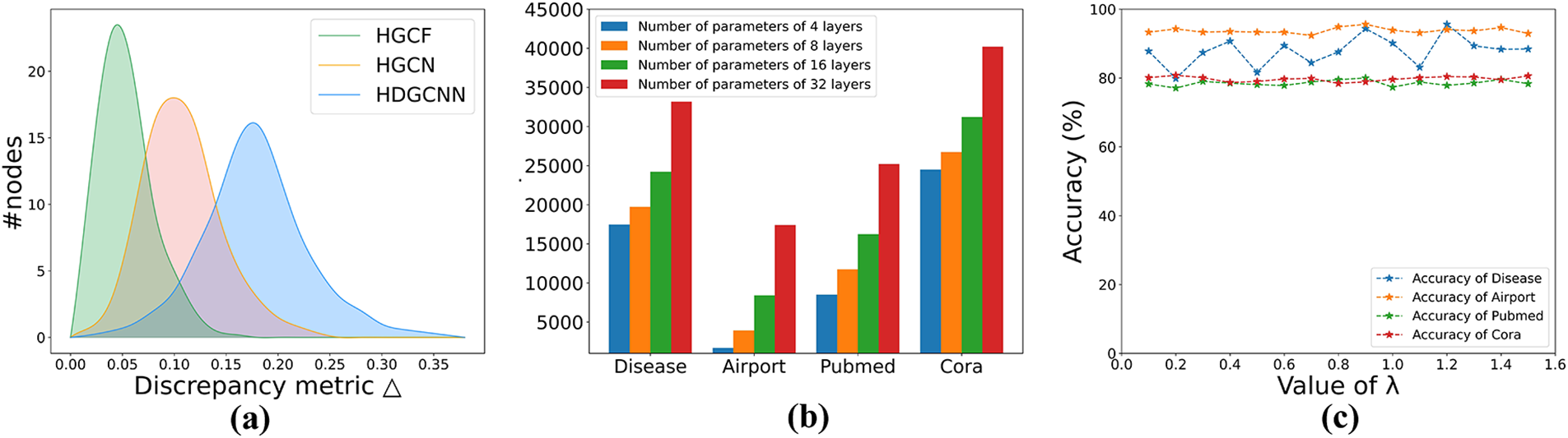
Figure 6: (a) Attention weight distribution on Airport; (b) The number of model parameters varies with the number of layers of the model; (c) Influence of hyperparameter λ on HDGCNN performance

5.5.2 Parameter Sensitivity Analysis

In this section, we will conduct a comprehensive sensitivity analysis to investigate the impact of the number of layers in HDGCNN on the total model parameters, as well as the influence of the adaptive decay parameter δl (as described in Eq. (11)) on the overall model performance. Fig. 6b depicts the variation in HDGCNN’s model parameters as the 4-layer model structure doubles to a 32-layer model across four datasets. Notably, the model parameters for the Disease, Pubmed, and Cora datasets do not exhibit a doubling pattern with the increase in the number of layers. Meanwhile, Fig. 6c depicts the fluctuations in node classification accuracy for the 32-layer HDGCNN across the four datasets as the hyperparameter λ within δl is adjusted. By manipulating the value of λ, the extent of information decay during the feature transformation stage can be controlled. It is evident from Fig. 6c that the performance of HDGCNN remains consistently stable within the λ range of 0.1 to 1.5. This resilience indicates the robustness and reliability of the model.

6  Conclusion

In this study, we introduced an end-to-end hyperbolic deep graph convolutional neural network model named HDGCNN for enhancing graph representation learning. This model was designed to effectively harness the structural insights of scale-free graphs featuring hierarchical arrangements, capturing extensive node dependencies, and extracting nuanced node features. Initially, we facilitated the seamless transition of input features from Euclidean space to hyperbolic space, thereby conserving the graph’s hierarchical structure with minimal distortion. This amalgamation of hyperbolic geometry and GCN yielded a potent framework for capturing both structural and node-specific attributes more efficiently. Subsequently, our proposed methodologies spanning feature transformation, neighborhood aggregation, and message passing stages contribute to the creation of a robust deep network architecture that circumvents over-smoothing issues. By capitalizing on the inherent strengths of this deep network structure, we adeptly grasp long-range dependencies among nodes and extract more intricate node features. Ultimately, our empirical findings underscore the remarkable superiority of HDGCNN over Euclidean GCN approaches and shallow hyperbolic graph neural networks, particularly when applied to graph datasets characterized by pronounced tree-like structures.

In the future, we intend to further investigate the effective integration of multi-dimensional edge feature learning within the framework of HDGCNN. This is driven by the realization that, in real-world graphs, aside from the potential manifestation of scale-free or hierarchical structural characteristics, edges also encompass a plethora of valuable features. Our aim in the forthcoming research is to explore how to concurrently embed scale-free or hierarchical graphs into hyperbolic space while efficiently acquiring multi-dimensional edge features, in order to enhance the precision of node feature learning.

Acknowledgement: We would like to express our sincere gratitude to Fanliang Bu for his valuable advice during the writing of our paper. In particular, we are thankful to Hongtao Huo for his guidance and assistance in preparing the manuscript. Furthermore, we appreciate the reviewers for their helpful suggestions, which have greatly improved the presentation of this paper.

Funding Statement: This work was supported by the National Natural Science Foundation of China-China State Railway Group Co., Ltd. Railway Basic Research Joint Fund (Grant No. U2268217) and the Scientific Funding for China Academy of Railway Sciences Corporation Limited (No. 2021YJ183).

Author Contributions: The authors confirm contribution to the paper as follows: study conception and design: Y.Z., F.B.; data collection: Z.H., H.H., X.L.; analysis and interpretation of results: L.B., Y.W., J.M.; draft manuscript preparation: Y.Z. All authors reviewed the results and approved the final version of the manuscript.

Availability of Data and Materials: The data that support the findings of this study are available from the first and corresponding authors upon reasonable request.

Conflicts of Interest: The authors declare that they have no conflicts of interest to report regarding the present study.

References

1. Zhou, J., Cui, G., Hu, S., Zhang, Z., Yang, C. et al. (2020). Graph neural networks: Review of methods and applications. AI Open, 1, 57–81. https://doi.org/10.1016/j.aiopen.2021.01.001 [Google Scholar] [CrossRef]

2. Wu, Z., Pan, S., Chen, F., Long, G., Zhang, C. et al. (2021). A comprehensive survey on graph neural networks. IEEE Transactions on Neural Networks and Learning Systems, 32(1), 4–24. https://doi.org/10.1109/TNNLS.2020.2978386 [Google Scholar] [PubMed] [CrossRef]

3. Chen, G., Guo, Y., Zeng, Q., Zhang, Y. (2023). A novel cellular network traffic prediction algorithm based on graph convolution neural networks and long short-term memory through extraction of spatial-temporal characteristics. Processes, 11(8), 2257. https://doi.org/10.3390/pr11082257 [Google Scholar] [CrossRef]

4. Zhang, Y. D., Satapathy, S. C., Guttery, D. S., Górriz, J. M., Wang, S. H. (2021). Improved breast cancer classification through combining graph convolutional network and convolutional neural network. Information Processing & Management, 58(2), 102439. https://doi.org/10.1016/j.ipm.2020.102439 [Google Scholar] [CrossRef]

5. Clauset, A., Moore, C., Newman, M. E. (2008). Hierarchical structure and the prediction of missing links in networks. Nature, 453(7191), 98–101. https://doi.org/10.1038/nature06830 [Google Scholar] [PubMed] [CrossRef]

6. Zitnik, M., Sosič, R., Feldman, M. W., Leskovec, J. (2019). Evolution of resilience in protein interactomes across the tree of life. Proceedings of the National Academy of Sciences, 116(10), 4426–4433. https://doi.org/10.1073/pnas.1818013116 [Google Scholar] [PubMed] [CrossRef]

7. Chen, W., Fang, W., Hu, G., Mahoney, M. W. (2013). On the hyperbolicity of small-world and tree-like random graphs. Internet Mathematics, 9(4), 434–491. https://doi.org/10.1080/15427951.2013.828336 [Google Scholar] [CrossRef]

8. Sala, F., De Sa, C., Gu, A., Ré, C., (2018). Representation tradeoffs for hyperbolic embeddings. International Conference on Machine Learning, pp. 4457–4466. Stockholm, Sweden. [Google Scholar]

9. Wu, S., Sun, F., Zhang, W., Xie, X., Cui, B. (2022). Graph neural networks in recommender systems: A survey. ACM Computing Surveys, 55(5), 1–37. https://doi.org/10.1145/3535101 [Google Scholar] [CrossRef]

10. Ni, Q., Ji, J. C., Halkon, B., Feng, K., Nandi, A. K. (2023). Physics-informed residual network (PIResNet) for rolling element bearing fault diagnostics. Mechanical Systems and Signal Processing, 200(2023), 110544. https://doi.org/10.1016/j.ymssp.2023.110544 [Google Scholar] [CrossRef]

11. Feng, K., Xu, Y., Wang, Y., Li, S., Jiang, Q. et al. (2023). Digital twin enabled domain adversarial graph networks for bearing fault diagnosis. IEEE Transactions on Industrial Cyber-Physical Systems, 1, 113–122. https://doi.org/10.1109/TICPS.2023.3298879 [Google Scholar] [CrossRef]

12. Li, Q., Han, Z., Wu, X. M. (2018). Deeper insights into graph convolutional networks for semi-supervised learning. Proceedings of the AAAI Conference on Artificial Intelligence, pp. 3538–3545. New Orleans, USA. [Google Scholar]

13. Kipf, T. N., Welling, M. (2017). Semi-supervised classification with graph convolutional networks. 5th International Conference on Learning Representations, pp. 1–14. Toulon, France. [Google Scholar]

14. Hamilton, W., Ying, Z., Leskovec, J. (2017). Inductive representation learning on large graphs. Advances in Neural Information Processing Systems, pp. 1024–1034. Long Beach, USA. [Google Scholar]

15. Zhang, M., Cui, Z., Neumann, M., Chen, Y. (2018). An end-to-end deep learning architecture for graph classification. Proceedings of the AAAI Conference on Artificial Intelligence, pp. 4438–4445. New Orleans, USA. [Google Scholar]

16. Ying, Z., You, J., Morris, C., Ren, X., Hamilton, W. et al. (2018). Hierarchical graph representation learning with differentiable pooling. Advances in Neural Information Processing Systems, pp. 4805–4815. Montréal, Canada. [Google Scholar]

17. Xu, K., Hu, W., Leskovec, J., Jegelka, S. (2018). How powerful are graph neural networks? arXiv: 1810.00826. [Google Scholar]

18. Schlichtkrull, M., Kipf, T. N., Bloem, P., Van Den Berg, R., Titov, I. et al. (2018). Modeling relational data with graph convolutional networks. The Semantic Web: 15th International Conference, pp. 593–607. Heraklion, Greece. [Google Scholar]

19. Nt, H., Maehara, T. (2019). Revisiting graph neural networks: All we have is low-pass filters. arXiv: 1905.09550. [Google Scholar]

20. Oono, K., Suzuki, T. (2020). Graph neural networks exponentially lose expressive power for node classification. 8th International Conference on Learning Representations, pp. 1–37. Addis Ababa, Ethiopia. [Google Scholar]

21. Alon, U., Yahav, E. (2021). On the bottleneck of graph neural networks and its practical implications. 9th International Conference on Learning Representations, pp. 1–37. Virtual Event. [Google Scholar]

22. Topping, J., di Giovanni, F., Chamberlain, B. P., Dong, X., Bronstein, M. M. (2021). Understanding over-squashing and bottlenecks on graphs via curvature. arXiv:2111.14522. [Google Scholar]

23. Deac, A., Lackenby, M., Veličković, P. (2022). Expander graph propagation. Learning on Graphs Conference, Virtual Event. [Google Scholar]

24. Li, G., Müller, M., Thabet, A. K., Ghanem, B. (2019). DeepGCNs: Can GCNs Go as deep as CNNs? Proceedings of the IEEE/CVF International Conference on Computer Vision, pp. 9266–9275. Seoul, South Korea. [Google Scholar]

25. He, K., Zhang, X., Ren, S., Sun, J. (2016). Deep residual learning for image recognition. Proceedings of the IEEE Conference on Computer Vision and Pattern Recognition, pp. 770–778. Las Vegas, USA. [Google Scholar]

26. Chen, M., Wei, Z., Huang, Z., Ding, B., Li, Y. (2020). Simple and deep graph convolutional networks. International Conference on Machine Learning, pp. 1725–1735. Virtual Event. [Google Scholar]

27. Xu, K., Li, C., Tian, Y., Sonobe, T., Kawarabayashi, K. I. et al. (2018). Representation learning on graphs with jumping knowledge networks. International Conference on Machine Learning, pp. 5453–5462. Stock, Sweden. [Google Scholar]

28. Zhao, L., Akoglu, L. (2020). PairNorm: Tackling over-smoothing in GNNs. 8th International Conference on Learning Representations, pp. 1–17. Addis Ababa, Ethiopia. [Google Scholar]

29. Zhou, K., Dong, Y., Wang, K., Lee, W. S., Hooi, B. et al. (2021). Understanding and resolving performance degradation in deep graph convolutional networks. Proceedings of the 30th ACM International Conference on Information & Knowledge Management, pp. 2728–2737. Queensland, Australia. [Google Scholar]

30. Li, G., Xiong, C., Thabet, A. K., Ghanem, B. (2020). DeeperGCN: All you need to train deeper GCNs. arXiv:2006.07739. [Google Scholar]

31. Zhou, K., Huang, X., Zha, D., Chen, R., Li, L. et al. (2021). Dirichlet energy constrained learning for deep graph neural networks. Advances in Neural Information Processing Systems, pp. 21834–21846. Virtual Event. [Google Scholar]

32. Rong, Y., Huang, W., Xu, T., Huang, J. (2020). DropEdge: Towards deep graph convolutional networks on node classification. 8th International Conference on Learning Representations, pp. 1–18. Addis Ababa, Ethiopia. [Google Scholar]

33. Huang, W., Rong, Y., Xu, T., Sun, F., Huang, J. (2020). Tackling over-smoothing for general graph convolutional networks. arXiv:2008.09864. [Google Scholar]

34. Ganea, O., Bécigneul, G., Hofmann, T. (2018). Hyperbolic neural networks. Advances in Neural Information Processing Systems, pp. 5350–5360. Montreal, Canada. [Google Scholar]

35. Nickel, M., Kiela, D. (2017). Poincaré embeddings for learning hierarchical representations. Advances in Neural Information Processing Systems, pp. 6338–6347. Long Beach, USA. [Google Scholar]

36. Katayama, K., Maina, E. W. (2015). Indexing method for hierarchical graphs based on relation among interlacing sequences of eigenvalues. Journal of Information Processing, 23(2), 210–220. https://doi.org/10.2197/ipsjjip.23.210 [Google Scholar] [CrossRef]

37. Yang, M., Li, Z., Zhou, M., Liu, J., King, I. (2022). HICF: Hyperbolic informative collaborative filtering. Proceedings of the 28th ACM SIGKDD Conference on Knowledge Discovery and Data Mining, pp. 2212–2221. Washington, USA. [Google Scholar]

38. Chen, Y., Yang, M., Zhang, Y., Zhao, M., Meng, Z. et al. (2022). Modeling scale-free graphs with hyperbolic geometry for knowledge-aware recommendation. Proceedings of the Fifteenth ACM International Conference on Web Search and Data Mining, pp. 94–102. Virtual Event. [Google Scholar]

39. Liu, Z., Li, X., You, Z., Yang, T., Fan, W. et al. (2021). Medical triage chatbot diagnosis improvement via multi-relational hyperbolic graph neural network. Proceedings of the 44th International ACM SIGIR Conference on Research and Development in Information Retrieval, pp. 1965–1969. Virtual Event. [Google Scholar]

40. Choudhary, N., Rao, N., Katariya, S., Subbian, K., Reddy, C. K. (2022). ANTHEM: Attentive hyperbolic entity model for product search. Proceedings of the Fifteenth ACM International Conference on Web Search and Data Mining, pp. 161–171. Virtual Event. [Google Scholar]

41. Wu, Z., Jiang, D., Hsieh, C. Y., Chen, G., Liao, B. et al. (2021). Hyperbolic relational graph convolution networks plus: A simple but highly efficient QSAR-modeling method. Briefings in Bioinformatics, 22(5), bbab112. https://doi.org/10.1093/bib/bbab112 [Google Scholar] [PubMed] [CrossRef]

42. Yu, K., Visweswaran, S., Batmanghelich, K. (2020). Semi-supervised hierarchical drug embedding in hyperbolic space. Journal of Chemical Information and Modeling, 60(12), 5647–5657. https://doi.org/10.1021/acs.jcim.0c00681 [Google Scholar] [PubMed] [CrossRef]

43. Tifrea, A., Bécigneul, G., Ganea, O. E. (2018). Poincaré glove: Hyperbolic word embeddings. arXiv:1810.06546. [Google Scholar]

44. Zhang, Y., Wang, X., Liu, N., Shi, C. (2022). Embedding heterogeneous information network in hyperbolic spaces. ACM Transactions on Knowledge Discovery from Data (TKDD), 16(2), 1–23. https://doi.org/10.1145/3468674 [Google Scholar] [CrossRef]

45. Chatterjee, S., Maheshwari, A., Ramakrishnan, G., Jagaralpudi, S. N. (2021). Joint learning of hyperbolic label embeddings for hierarchical multi-label classification. arXiv:2101.04997. [Google Scholar]

46. Wang, S., Kang, Q., She, R., Wang, W., Zhao, K. et al. (2023). HypLiLoc: Towards effective LiDAR pose regression with hyperbolic fusion. Proceedings of the IEEE/CVF Conference on Computer Vision and Pattern Recognition, pp. 5176–5185. Vancouver, Canada. [Google Scholar]

47. Ermolov, A., Mirvakhabova, L., Khrulkov, V., Sebe, N., Oseledets, I. (2022). Hyperbolic vision transformers: Combining improvements in metric learning. Proceedings of the IEEE/CVF Conference on Computer Vision and Pattern Recognition, pp. 7409–7419. New Orleans, USA. [Google Scholar]

48. Zhang, C., Gao, J., (2021). Hype-HAN: Hyperbolic hierarchical attention network for semantic embedding. Proceedings of the Twenty-Ninth International Conference on International Joint Conferences on Artificial Intelligence, pp. 3990–3996. Yokohama, Japan. [Google Scholar]

49. Do Carmo, M. P., Flaherty Francis, J. (1992). Riemannian geometry. Boston: Birkhäuser. [Google Scholar]

50. Nickel, M., Kiela, D. (2018). Learning continuous hierarchies in the lorentz model of hyperbolic geometry. Proceedings of the 35th International Conference on Machine Learning, pp. 3776–3785. Stockholm, Sweden. [Google Scholar]

51. Klicpera, J., Bojchevski, A., Günnemann, S. (2019). Predict then propagate: Graph neural networks meet personalized PageRank. 7th International Conference on Learning Representations, pp. 1–15. New Orleans, USA. [Google Scholar]

52. He, X., Deng, K., Wang, X., Li, Y., Zhang, Y. et al. (2020). LightGCN: Simplifying and powering graph convolution network for recommendation. Proceedings of the International ACM SIGIR Conference on Research and Development in Information Retrieval, pp. 639–648. Virtual Event. [Google Scholar]

53. Liu, Q., Nickel, M., Kiela, D. (2019). Hyperbolic graph neural networks. Advances in Neural Information Processing Systems, pp. 8230–8241. Vancouver, Canada. [Google Scholar]

54. Zhang, Y., Wang, X., Shi, C., Jiang, X., Ye, Y. (2021). Hyperbolic graph attention network. IEEE Transactions on Big Data, 8(6), 1690–1701. https://doi.org/10.1109/TBDATA.2021.3081431 [Google Scholar] [CrossRef]

55. Chami, I., Ying, Z., Ré, C., Leskovec, J. (2019). Hyperbolic graph convolutional neural networks. Advances in Neural Information Processing Systems, pp. 4868–4879. Vancouver, Canada. [Google Scholar]

56. Veličković, P., Cucurull, G., Casanova, A., Romero, A., Lio, P. et al. (2018). Graph attention networks. 6th International Conference on Learning Representations, pp. 1–12. Vancouver, Canada. [Google Scholar]

57. Huang, G., Liu, Z., van der Maaten, L., Weinberger, K. Q. (2017). Densely connected convolutional networks. Proceedings of the IEEE Conference on Computer Vision and Pattern Recognition, pp. 4700–4708. Honolulu, USA. [Google Scholar]

58. Adcock, A. B., Sullivan, B. D., Mahoney, M. W. (2013). Tree-like structure in large social and information networks. 2013 IEEE 13th International Conference on Data Mining, pp. 1–10. Dallas, USA. [Google Scholar]

59. Anderson, R. M., May, R. M. (1991). Infectious diseases of humans: Dynamics and Control. Oxford: Oxford University Press. [Google Scholar]

60. Sen, P., Namata, G., Bilgic, M., Getoor, L., Galligher, B. et al. (2008). Collective classification in network data. AI Magazine, 29(3), 93–106. https://doi.org/10.1609/aimag.v29i3.2157 [Google Scholar] [CrossRef]

61. Wu, F., Souza, A., Zhang, T., Fifty, C., Yu, T. et al. (2019). Simplifying graph convolutional networks. International Conference on Machine Learning, pp. 6861–6871. California, USA. [Google Scholar]

62. Gulcehre, C., Denil, M., Malinowski, M., Razavi, A., Pascanu, R. et al. (2019). Hyperbolic attention networks. Proceedings of the 7th International Conference on Learning Representations, pp. 1–15. New Orleans, USA. [Google Scholar]

63. Sun, J., Cheng, Z., Zuberi, S., Pérez, F., Volkovs, M. (2021). HGCF: Hyperbolic graph convolution networks for collaborative filtering. Proceedings of the Web Conference 2021, pp. 593–601. Virtual Event. [Google Scholar]

64. Yang, Z., Cohen, W., Salakhudinov, R. (2016). Revisiting semi-supervised learning with graph embeddings. International Conference on Machine Learning, pp. 40–48. New York, USA. [Google Scholar]

65. Kingma, D. P., Ba, J. (2015). Adam: Method for stochastic optimization. 3rd International Conference on Learning Representations, pp. 1–15. San Diego, USA. [Google Scholar]

66. Chen, D., Lin, Y., Li, W., Li, P., Zhou, J. et al. (2020). Measuring and relieving the over-smoothing problem for graph neural networks from the topological view. Proceedings of the AAAI Conference on Artificial Intelligence, pp. 3438–3445. New York, USA. [Google Scholar]

67. Shanthamallu, U. S., Thiagarajan, J. J., Spanias, A. (2020). A regularized attention mechanism for graph attention networks. 2020 IEEE International Conference on Acoustics, Speech and Signal Processing (ICASSP), pp. 3372–3376. Barcelona, Spain. [Google Scholar]