
 Submit a Paper
 Propose a Special lssue
 Open Access
ARTICLE

Fast and Accurate Predictor-Corrector Methods Using Feedback-Accelerated Picard Iteration for Strongly Nonlinear Problems
1 School of Astronautics, Northwestern Polytechnical University, Xi’an, 710072, China
2 Department of Mechanical Engineering, Texas Tech University, Lubbock, 79409, USA
* Corresponding Author: Wei He. Email:
Computer Modeling in Engineering & Sciences 2024, 139(2), 1263-1294. https://doi.org/10.32604/cmes.2023.043068
Received 20 June 2023; Accepted 27 October 2023; Issue published 29 January 2024
 View Full Text
 Download PDF
Abstract
Although predictor-corrector methods have been extensively applied, they might not meet the requirements of practical applications and engineering tasks, particularly when high accuracy and efficiency are necessary. A novel class of correctors based on feedback-accelerated Picard iteration (FAPI) is proposed to further enhance computational performance. With optimal feedback terms that do not require inversion of matrices, significantly faster convergence speed and higher numerical accuracy are achieved by these correctors compared with their counterparts; however, the computational complexities are comparably low. These advantages enable nonlinear engineering problems to be solved quickly and accurately, even with rough initial guesses from elementary predictors. The proposed method offers flexibility, enabling the use of the generated correctors for either bulk processing of collocation nodes in a domain or successive corrections of a single node in a finite difference approach. In our method, the functional formulas of FAPI are discretized into numerical forms using the collocation approach. These collocated iteration formulas can directly solve nonlinear problems, but they may require significant computational resources because of the manipulation of high-dimensional matrices. To address this, the collocated iteration formulas are further converted into finite difference forms, enabling the design of lightweight predictor-corrector algorithms for real-time computation. The generality of the proposed method is illustrated by deriving new correctors for three commonly employed finite-difference approaches: the modified Euler approach, the Adams-Bashforth-Moulton approach, and the implicit Runge-Kutta approach. Subsequently, the updated approaches are tested in solving strongly nonlinear problems, including the Matthieu equation, the Duffing equation, and the low-earth-orbit tracking problem. The numerical findings confirm the computational accuracy and efficiency of the derived predictor-corrector algorithms.Graphic Abstract
Keywords
In real-world engineering tasks and scientific research, predictor-corrector methods are fundamental to numerically solving nonlinear differential equations [1–3]. Currently, there are hundreds of variants of these methods, which often involve the use of explicit formulas to obtain rough predictions and implicit formulas for further corrections. In general, the predictor-corrector method is widely used in asymptotic and weighted residual methods. This study focuses on finite difference approaches, in which correctors are typically employed once per step. Although multiple corrections can enhance computational accuracy, this approach significantly slows down the algorithm. Therefore, the preference is to reduce the step size rather than repeat corrections. Conventional correctors are often derived from Picard iteration (PI) to solve nonlinear algebraic equations (NAEs) associated with implicit formulas [4,5]. Despite their ease of implementation, these correctors may be insufficient in generating accurate results and ensuring the reliability of long-term simulations for strongly nonlinear dynamical systems. In practical applications, it can result in destructive time delays in tasks that aim for highly accurate results, or it can fail to achieve highly accurate results in real-time computation. Such instances are found in large-scale dynamics simulations [6], autonomous navigation [7], and path-tracking control [8].
This study presents three main contributions. First, an approach to derive fast and accurate correctors to enhance the performance of predictor-corrector methods for more advanced tasks in real life is proposed. This is achieved by replacing PI with feedback-accelerated Picard iteration (FAPI) [9]. These two iteration approaches are categorized as asymptotic approaches that iteratively solve analytical solutions of nonlinear systems starting from an initial guess [10]. The authors in [11] have demonstrated that PI can be considered a special case of FAPI. The latter approach is based on the concept of correcting an approximated solution through the integration of an optimally weighted residual function. FAPI degenerates into PI if the optimal weighting function is specified as a unit matrix instead of being derived from the optimal condition [12]. Therefore, FAPI converges faster and is more stable. Second, since FAPI cannot be employed directly to solve NAEs, the iterative formula is further discretized with appropriate basis functions and collocation nodes [13] to obtain numerical correctors corresponding to PI and FAPI. The PI correctors obtained in this method are equivalent to conventional correctors that directly employ PI to solve implicit finite difference formulas. Third, the proposed approach can be directly applied to other existing predictor-corrector approaches to enhance performance.
The applications of the enhanced predictor-corrector methods and FAPI span various domains, including simulations of n-body problems in celestial mechanics [6], molecular dynamics [14], high-dimensional nonlinear structural dynamics [15], and other problems in fluid mechanics, solid mechanics, heat transfer, and related areas. Particularly, these methods can offer straightforward applications in aerospace engineering for the accurate on-board prediction of spacecraft flight trajectories to achieve autonomous precision navigation [7].
This study is structured as follows. In Section 2, the relationship between PI and FAPI is revealed, and the methodology is introduced by constructing numerical correctors from the discretized collocation formulas of FAPI, which are derived for a general nonlinear dynamical system. Section 3 briefly reviews the underlying relationship between finite difference and collocation, followed by the derivation of FAPI correctors corresponding to three classical finite difference approaches: the modified Euler approach [16], the Adams-Bashforth-Moulton approach [17], and the implicit Runge-Kutta approach [18]. In Section 4, three nonlinear problems (the Matthieu equation [19], the Duffing equation [20], and the low-earth-orbit (LEO) tracking problem [21]) are used as numerical examples to verify the effectiveness of the proposed FAPI correctors.
Consider a nonlinear dynamical system in the form of
Without loss of generality, we suppose
It can be rewritten as
where
Suppose
Let
Now we want to make all the components of the function
Then we collect the terms including
Note that the boundary value of
from which we can derive the first order appoximation of
where J is the Jacobian matrix of
which means the error caused will not exceed
By substituting Eq. (10) into Eq. (4), the correctional formula becomes
where
Previously, the formula of FAPI takes the form of Eq. (12). In this work, we propose another form of it. By differentiating Eq. (4), we have
with Eqs. (9), (13) can be rewritten as
Simply approximating
By integrating both sides of Eq. (15), we have
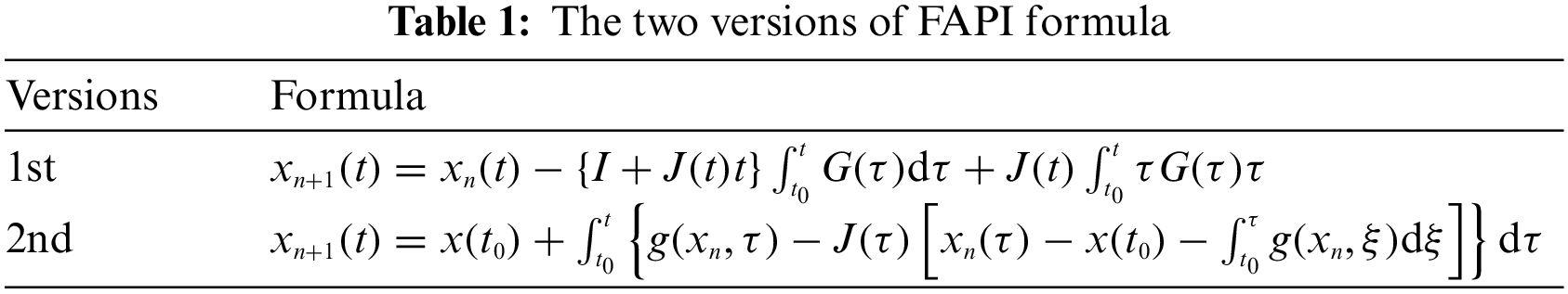
For clarity, the two versions of FAPI fomulae are listed in Table 1.
2.2.1 The 1st Version of Collocated FAPI
By collocating M nodes in time domain, Eq. (12) can be discretized. It is written as
The block diagonal matrices
We suppose that
Using the approximation in Eq. (19), it is obtained that
where
Further, by making the basis functions in Eq. (19) universal, it is found that
where the integration matrix
For simplicity, we denote
However, it may cause deterioration of the numerical solution, because
where the modified integration matrix
Denoting
We further denote the constant matrix
where
2.2.2 The 2nd Version of Collocated FAPI
Further numerical discretization is made to the collocation form of Eq. (15). It is expressed as
In Eq. (30),
We suppose that
Similar approximations can be made to the components
Using the approximations in Eqs. (32), (33), it is obtained that
and
where the integration matrix
For simplicity, we denote
where
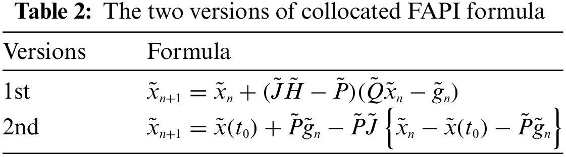
For clarity, the two versions of collocated FAPI formulae are displayed in Table 2.
2.3 FAPI as Numerical Corrector
Each row of Eqs. (29) or (37) can be used independently as a numerical corrector. For instance, the last row of Eq. (37) can be written as
where the superscript M of matrices
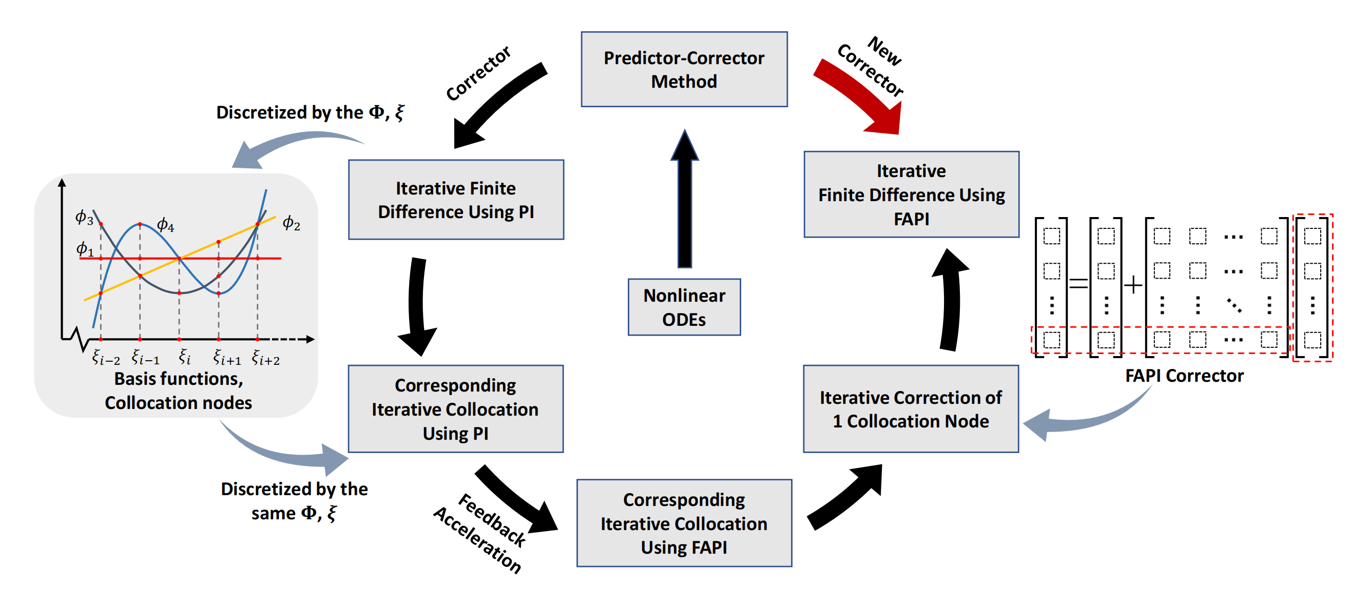
Given the values of collocation nodes
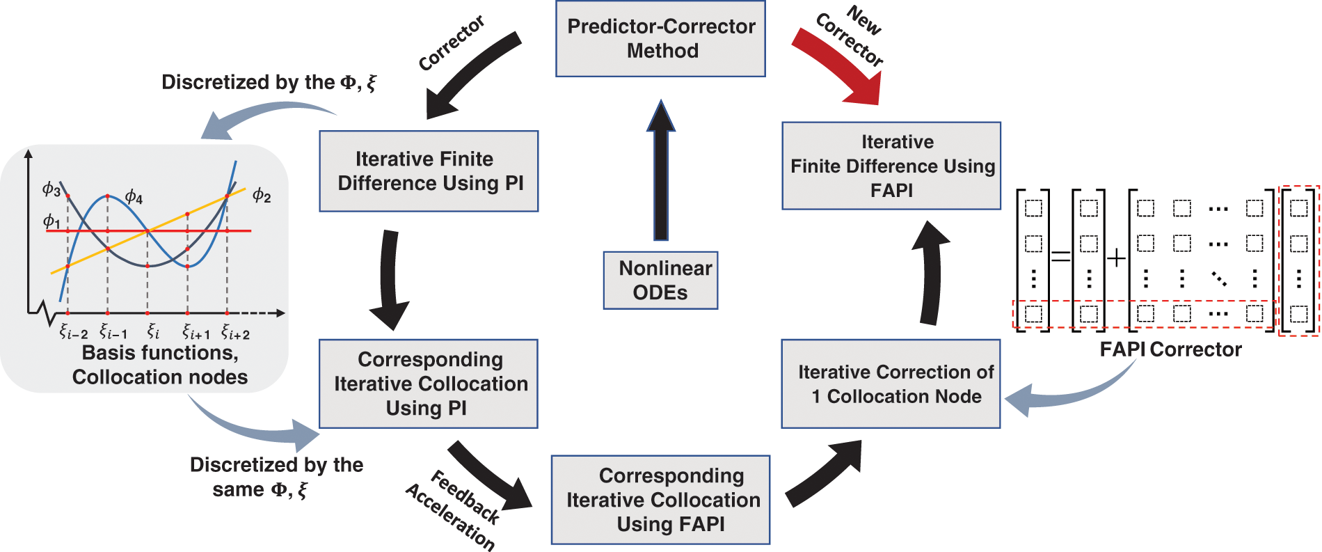
Figure 1: The process to derive FAPI corrector for predictor-corrector method when dealing general nonlinear ODEs
3 Finite Difference Integrators Featured by FAPI
To apply FAPI as numerical corrector in finite difference method, we need to use the same collocation nodes and basis functions underlying the finite difference discretization. The relationship between finite difference and collocation is briefly reviewed herein.
3.1 From Collocation to Finite Difference
The collocation form of Eq. (1) can be written as
where
Eq. (40) is a finite difference form of Eq. (1). If
Besides, Eq. (1) can be equivalently expressed as
The collocation form of Eq. (41) is
where
It is an implicit finite difference formula. Usually, we let
Since Eqs. (43) and (40) are obtained by numerical differentiation and integration, respectively, using collocation method, we can find the counterpart of a finite difference method as a collocation method by choosing proper basis functions and collocation nodes, or derive a finite difference formula from collocation method.
3.2 Modified Euler Method Using FAPI
Herein, we consider the Modified Euler method (MEM) that only uses 2 nodes, of which one is known and the other is unknown. The collocation counterpart of this method has 2 collocation nodes, and takes the Lagrange polynomials
and
By substituting Eq. (45) into Eq. (39), we have
The first row of Eq. (46) is an explicit formula of Euler method, while the second row is implicit. They can be used independently or conjointly in a predictor-corrector manner. In the later case, the explicit formula provides prediction for the implicit formula to make further correction. Usually, the correction is made by the Picard iteration method due to its low computational complexity and inversion-free property. Based on Eq. (46), a predictor-corrector formula using Picard iteration can thus be expressed as
where
However, the modified Euler method utilizes the trapezoidal formula instead of the implicit Euler formula to make correction. The trapezoidal formula can be derived from Eq. (42). By using the same collocation nodes and basis functions that lead to Eq. (46), we have
and
Note that we start the integration at
The second row of Eq. (51) is the formula of trapezoidal method. Given
Eqs. (47) and (52) constitute the modified Euler method.
3.2.1 The 1st Version of ME-FAPI Method
Now we replace Eq. (52) with the feedback-accelerated Picard iteration. The necessary matrices are derived first as following:
With Eqs. (50) and (53),
Thus
According to Eq. (29), we have
It is rewritten as
where
3.2.2 The 2nd Version of ME-FAPI Method
According to Eq. (37), we have
It is rewritten as
where
3.3 Adams-Bashforth-Moulton Method Using FAPI
Taking the 4-th order Adams-Bashforth-Moulton (ABM) method for instance, it solves Eq. (1) with the following formula:
of which Eq. (60) is a predictor using an Adams-Bashforth formula and Eq. (61) is a corrector that uses Picard iteration to solve an Adams-Moulton formula.
3.3.1 The 1st Version of ABM-FAPI Method
To replace the Picard iteration with Feedback-Accelerated Picard iteration in the Adams-Moulton corrector (Eq. (61)), we only need to determine the differentiation matrix
With Eq. (62), the differentiation matrix
To keep consistent with the Adams-Moulton formula underlying Eq. (61), we let the integration in Eq. (12) start from
and
They are further expressed as
and
Then the matrix
The matrix
By substituting Eqs. (63) and (69) into Eq. (29), we have
It is explicitly expressed as
where the terms related with
3.3.2 The 2nd Version of ABM-FAPI Method
According to Eq. (37), we have
It is rewritten as
3.4 Implicit Runge-Kutta Method Using FAPI
The equivalence between implicit Runge-Kutta (IRK) method and collocation method has been well discussed and proved [22]. For that, the collocated FAPI provides iterative formulae for implicit Runge-Kutta methods. A 4-stage implicit Runge-Kutta method is taken as an example, where its corresponding collocation method takes the first kind of Chebyshev polynomials and Chebyshev-Gauss-Lobatto (CGL) nodes as basis functions and collocation nodes, respectively.
By re-scaling the time segment as
where
From Eqs. (23) and (26), the integration matrices
The 4-stage implicit Runge-Kutta method using Picard iteration is expressed as
3.4.1 The 1st Version of IRK-FAPI Method
By substituting Eqs. (75)–(77) into the 1st collocated FAPI formula
where
3.4.2 The 2nd Version of IRK-FAPI Method
The 2nd version of the 4-stage IRK-FAPI formula can be obtained by substituting Eq. (76) into the 2nd collocated FAPI formula as following:
4 Numerical Results and Discussion
In this section, conventional predictor-corrector methods, the corresponding FAPI enhanced methods, and MATLAB-built-in ode45/ode113 were used to solve the dynamical responses of some typical nonlinear systems, such as the Mathieu equation, the forced Duffing equation, and the perturbed two-body problem. The numerical simulation was conducted in MATLAB R2017a using an ASUS laptop with an Intel Core i5-7300HQ CPU. GPU acceleration and parallel processing were not used in the following examples.
In this study, to conduct a comprehensive and rational evaluation of each approach, two approaches were employed to compare the accuracy, convergence speed, and computational efficiency of conventional approaches and the corresponding FAPI-enhanced methods. The first approach involves performing the iterative correction only once, which is the general usage of the prediction-correction algorithm. The second approach involves repeating the iterative correction until the corresponding terminal conditions are met.
The maximum computational error in the simulation time interval was selected to represent the computational accuracy when evaluating the computational accuracy of each approach. The solution of ode45 or ode113 was employed as the benchmark for calculating this computational error. The relative and absolute errors of ode45 and ode113 were set as
Mathieu Equation
The Mathieu equation is
where the parameters are set as
Forced Duffing Equation
The forced Duffing equation is
where the parameters are set as
Low-Earth-Orbit Tracking Problem
The orbital problem is considered in the following form:
where
The computational accuracy of orbital motion plays a crucial role in determining the success of space missions. In the case of LEO, the long-term trajectory of a spacecraft can be significantly affected by a very small perturbation term of gravity force. A high-order gravitational model should be used to achieve relatively high accuracy. In this case, most computational time is dedicated to assessing the gravitational force terms. The relative error of position is defined as
4.1 Modified Euler Method Using FAPI
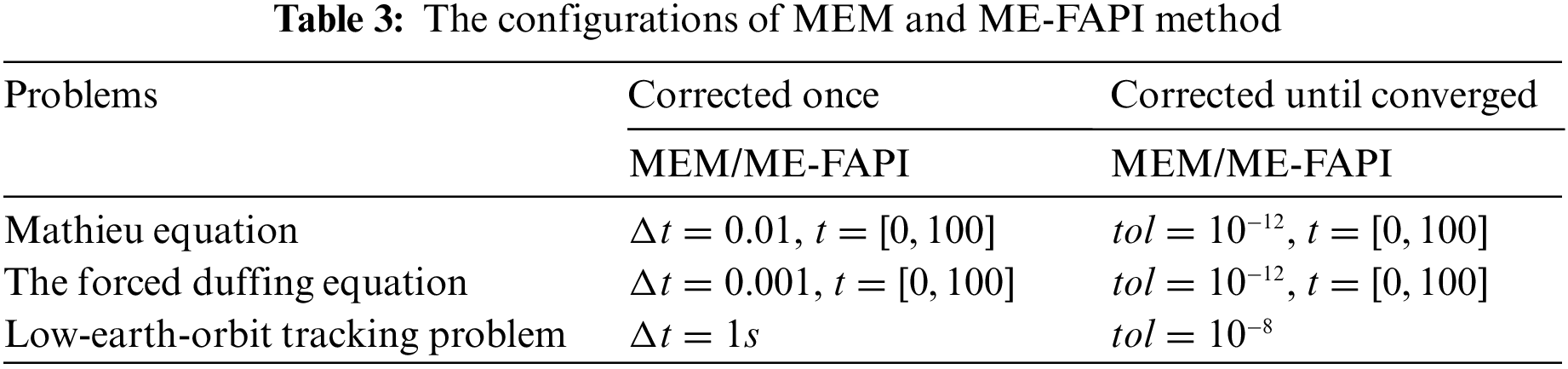
Using ode45/ode113 as the benchmark, Figs. 2 and 3 show a straightforward comparison of the phase plane portraits, time responses, and computational errors of MEM, 1st ME-FAPI, and 2nd ME-FAPI when solving the Matthieu and forced Duffing equations. Fig. 4 shows a comparison of the trajectory of LEO and the computational errors. Table 3 presents the time step size of each method.
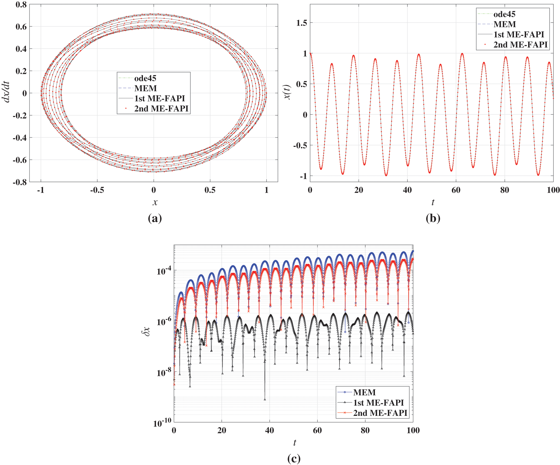
Figure 2: Results of Mathieu equation using MEM, ME-FAPI, and ode45: (a) phase plane portrait; (b) time responses; (c) computational error
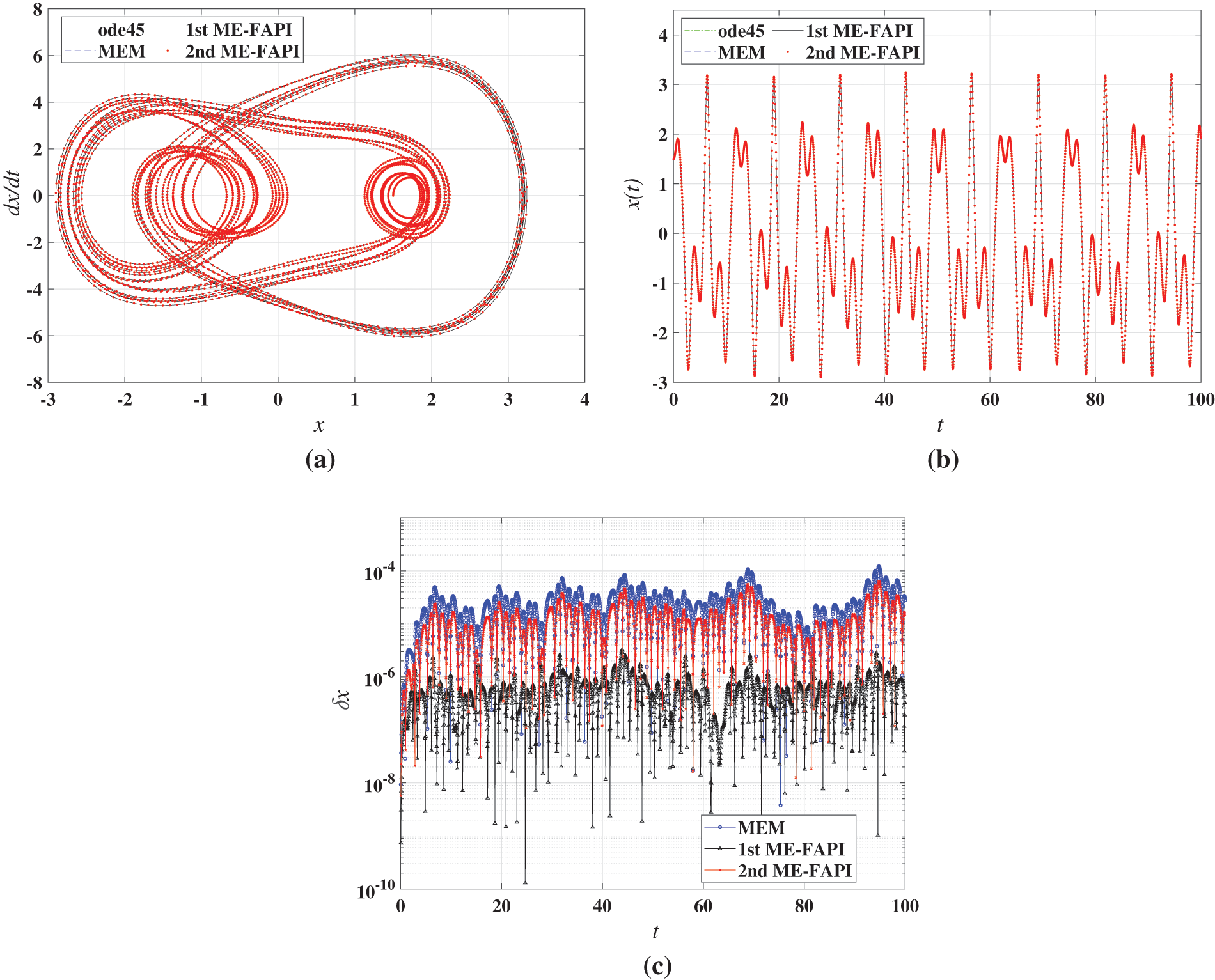
Figure 3: Results of the forced duffing equation using MEM, ME-FAPI, and ode45: (a) phase plane portrait; (b) time responses; (c) computational error
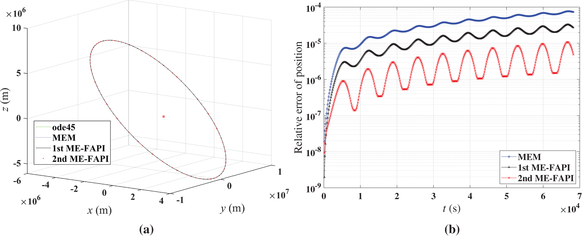
Figure 4: Results of MEM, ME-FAPI, and ode113 for LEO: (a) trajectory of LEO; (b) computational error
The MEM and ME-FAPI methods exhibited a good match with ode45/ode113. In Fig. 2c, the error curve of the 1st ME-FAPI method is relatively steady, whereas the error curves of the 2nd ME-FAPI method and MEM gradually increase with time. This indicates that the 1st ME-FAPI method has a significantly lower error accumulation rate than the 2nd ME-FAPI method and MEM when solving the Mathieu equation. In the numerical results of the Duffing equation, an improvement in computational accuracy with the 1st ME-FAPI method is also observed. The error curve of the LEO tracking problem in Fig. 4b shows a significant correlation with the current orbital position (or altitude) of the satellite, which is due to the strong association between the macroscopic gravity field and the orbital position (altitude). This observation reveals that the 2nd ME-FAPI method is more accurate in solving the orbit tracking problem.
A more comprehensive presentation of the computational accuracy and efficiency of each method is shown in Figs. 5–7 when the proposed ME-FAPI method and MEM are only corrected once. The maximum computational error of each method was recorded by sweeping the time step size
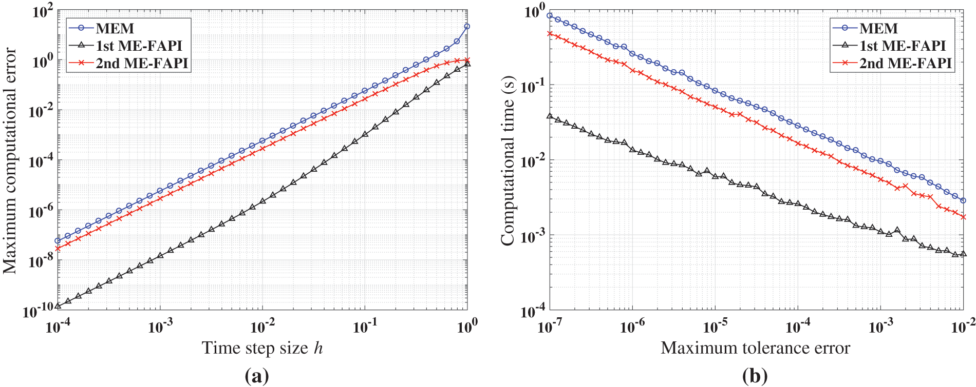
Figure 5: Performance of MEM and ME-FAPI in solving Mathieu equation when corrected only once: (a) Maximal error; (b) computational time
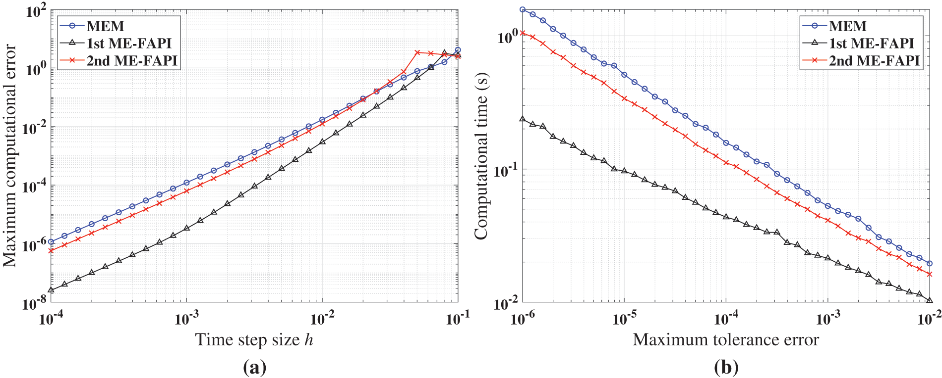
Figure 6: Performance of MEM, and ME-FAPI in solving the forced Duffing equation when corrected only once: (a) Maximal error; (b) computational time
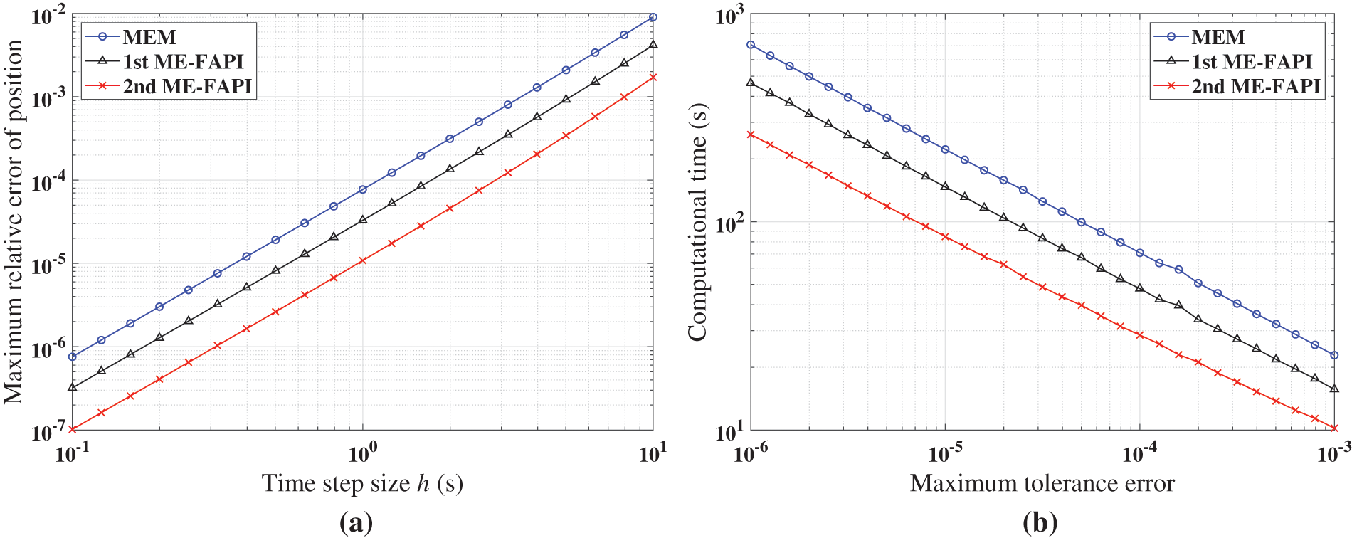
Figure 7: Performance of MEM, and ME-FAPI for LEO when corrected only once: (a) Maximal error; (b) computational time
Figs. 5–7 demonstrate that the ME-FAPI method proposed in this study outperforms MEM when corrected once in terms of accuracy and efficiency. The two versions of the ME-FAPI method have varying applicability for different nonlinear systems. For instance, the 1st ME-FAPI method is more suitable for solving the Mathieu equation, where its computational error is 1–2 magnitudes lower than that of the MEM, and its computational time is only
The following section examines the performance indices of each approach after the convergence of the iterative process, including the maximum computational error, average iteration steps, and computational efficiency. Table 3 presents the configurations of these methods, and Figs. 8–10 illustrate the simulation results. Since the convergence speed of each method shows similar rules in different cases, only the corresponding simulation results of the Mathieu equation are retained.
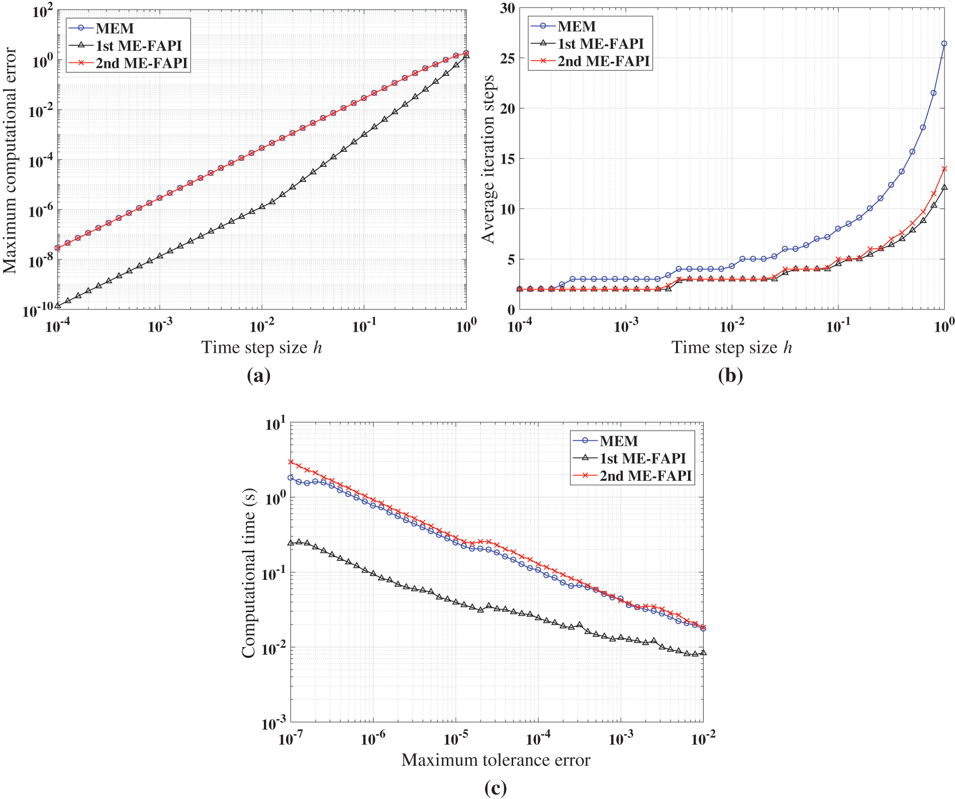
Figure 8: Performance of MEM, and ME-FAPI in solving Mathieu equation when the algorithms converge: (a) Maximal error; (b) average iteration steps; (c) computational time
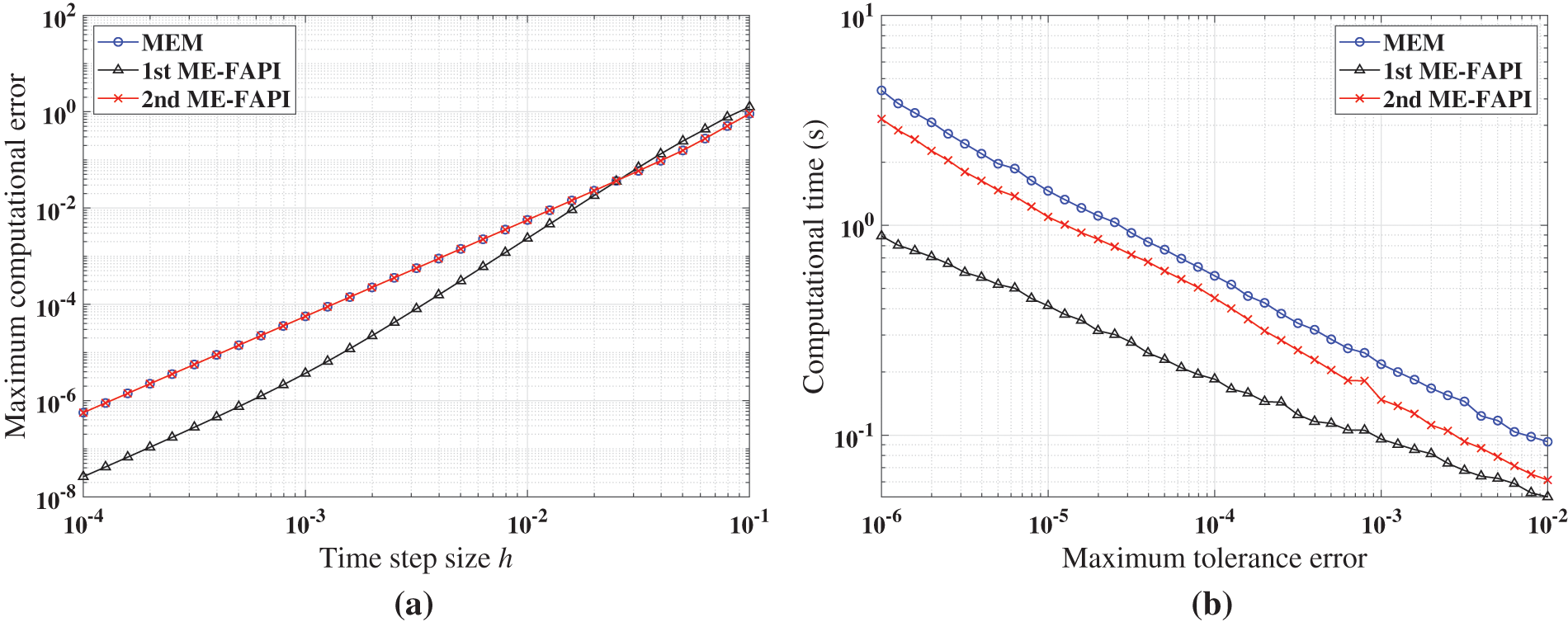
Figure 9: Performance of MEM, and ME-FAPI in solving the forced duffing equation when the algorithms converge: (a) Maximal error; (b) computational time
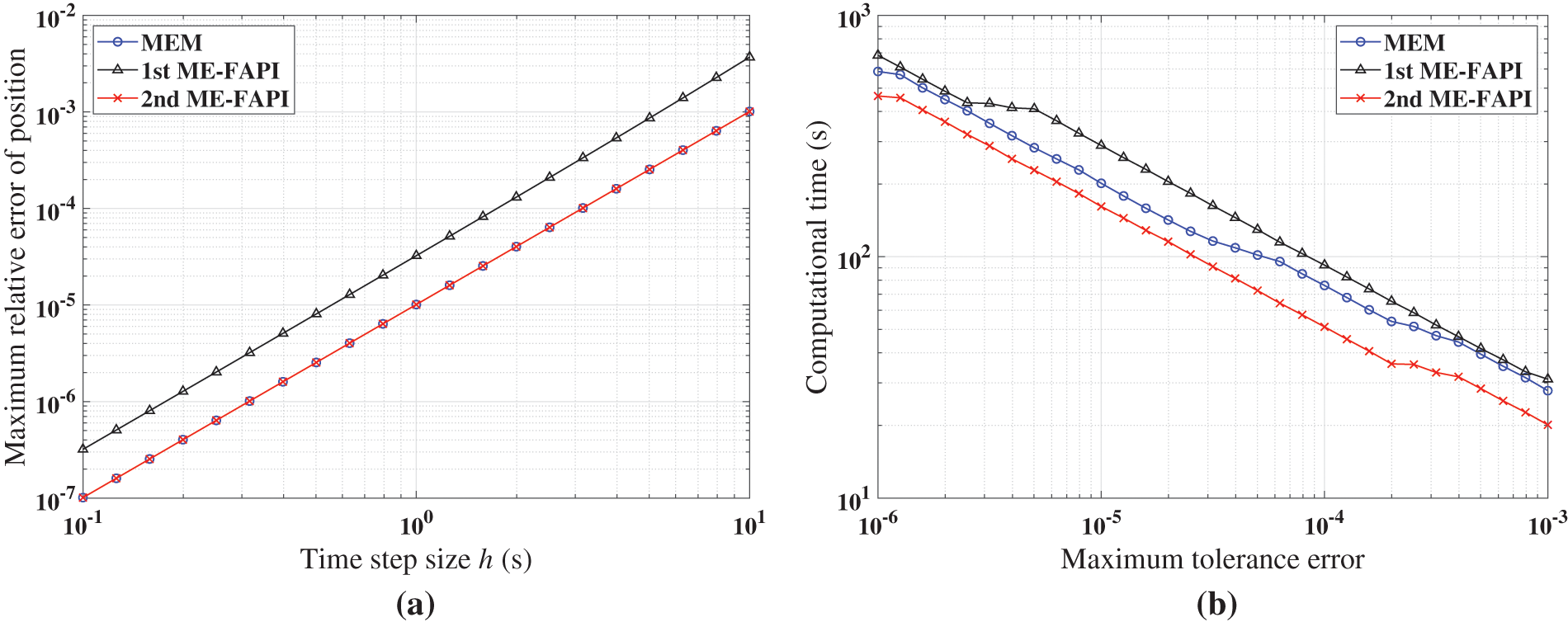
Figure 10: Performance of MEM, and ME-FAPI for LEO when the algorithms converge: (a) Maximal error; (b) computational time
Figs. 8–10 demonstrate that at least one of the two versions of the ME-FAPI method proposed in this study will have higher computational efficiency than the classical MEM. Only the 1st ME-FAPI method is more efficient than MEM when solving the Mathieu equation, as illustrated in Fig. 8. However, the 1st and 2nd ME-FAPI methods are more efficient than MEM when solving the Duffing equation. Thus, in practical applications, it is crucial to select the appropriate approach based on the specific problem to be solved.
Furthermore, Fig. 8b illustrates that the 1st ME-FAPI and 2nd ME-FAPI methods converge almost as fast, while the MEM method exhibits the slowest convergence. The advantage of convergence speed substantially enhances the efficiency of the method. For instance, the evaluations of the force model consume most of the computational time when solving the perturbed two-body problem. Therefore, a reduction in the number of iterations plays a significant role in reducing computational cost.
4.2 Adams-Bashforth-Moulton Method Using FAPI
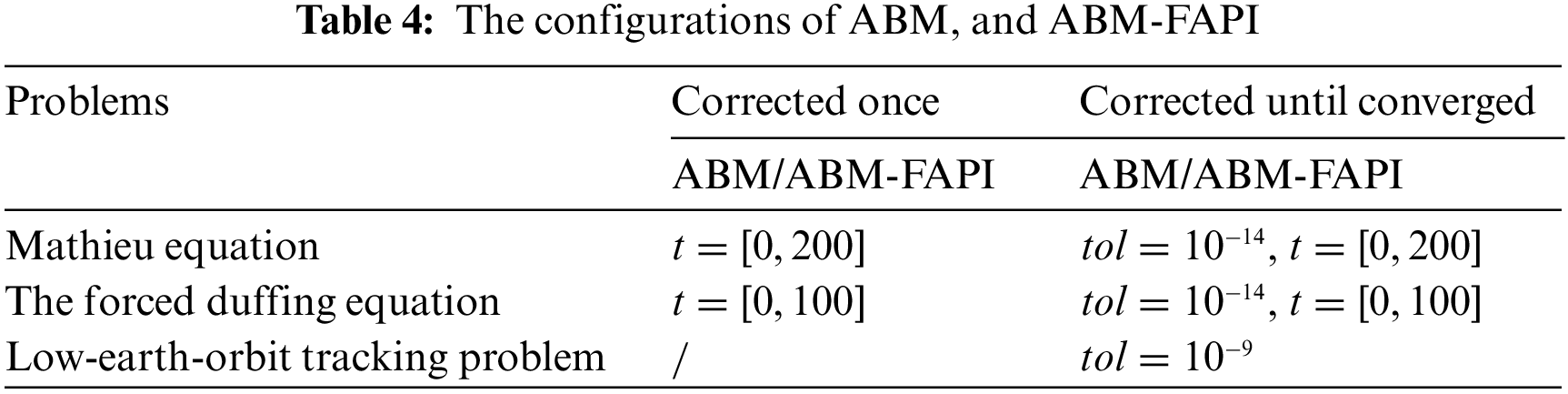
When corrected only once, the simulation results in Figs. 11–13 provide an overview of the computational accuracy and efficiency of each method. Table 4 shows the duration of the simulated dynamical response.
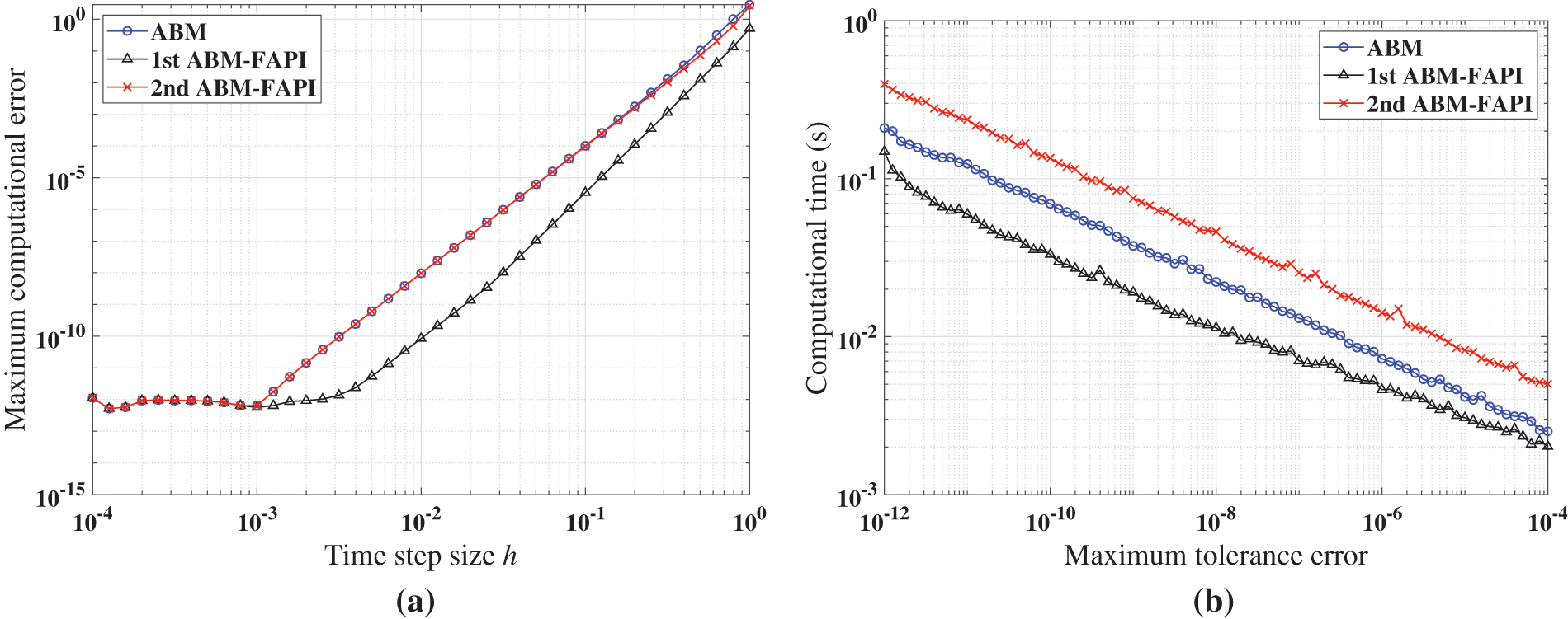
Figure 11: Performance of ABM, and ABM-FAPI in solving Mathieu equation when corrected only once: (a) Maximal error; (b) computational time
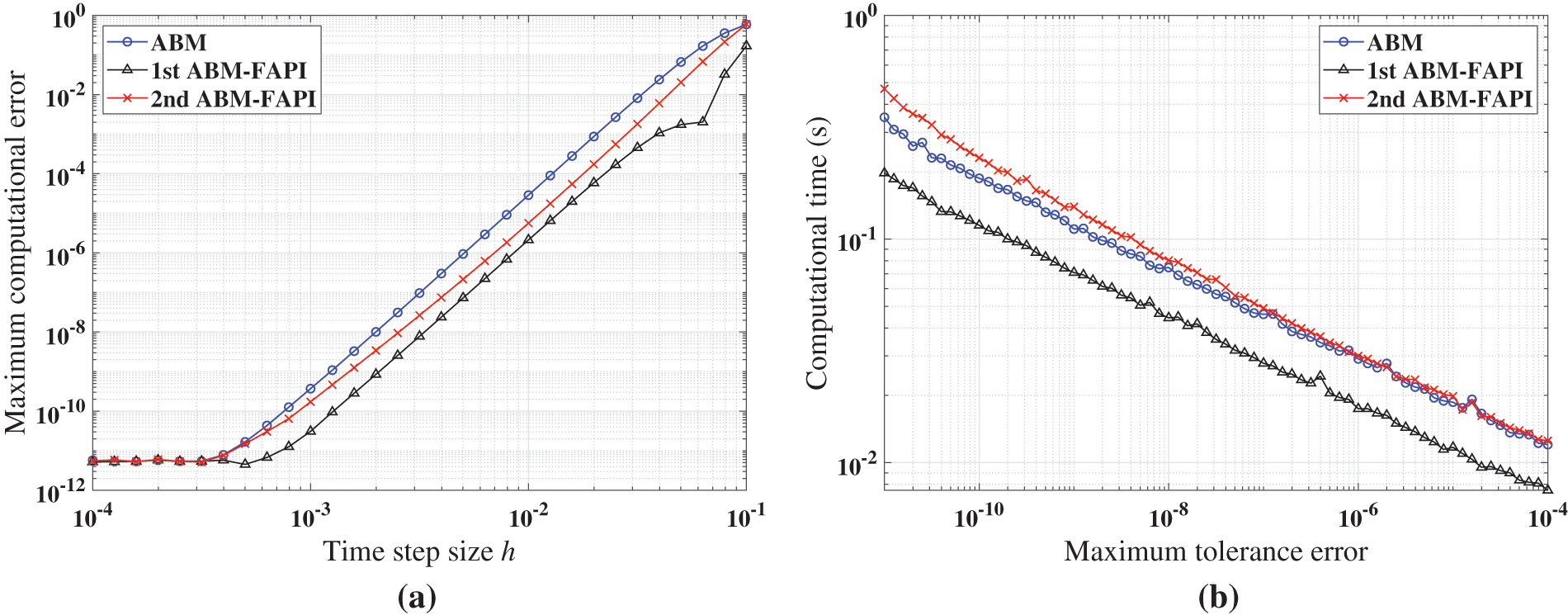
Figure 12: Performance of ABM, and ABM-FAPI in solving the forced Duffing equation when corrected only once: (a) Maximal error; (b) computational time
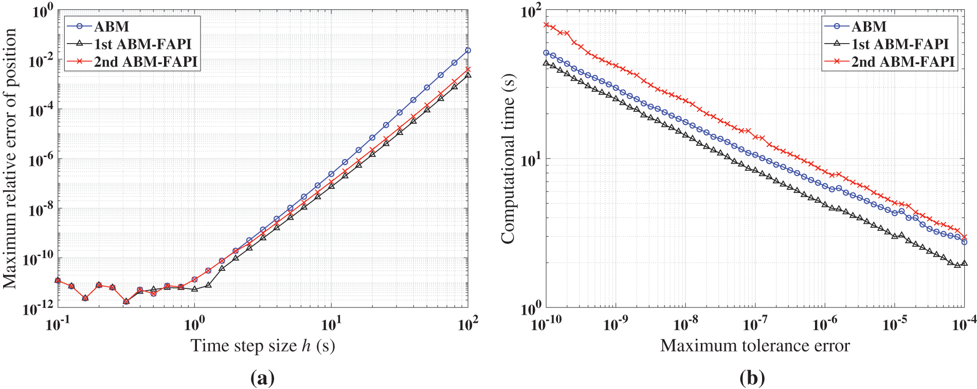
Figure 13: Performance of ABM, and ABM-FAPI for LEO when corrected only once: (a) Maximal error; (b) computational time
Figs. 11–13 demonstrate that when corrected only once, the 1st ABM-FAPI method is more accurate and efficient than the ABM method in all cases. For instance, the computational error of the 1st ABM-FAPI method is 1–2 orders of magnitude lower than that of the ABM method at the same step size when solving the Mathieu equation (Fig. 11). Furthermore, at the same computational accuracy, the former can save approximately
New results can be obtained when the algorithms converge, as shown in Figs. 14–16. Table 4 shows the configurations of these methods. For the same reason as in the previous section, only the simulation results of the Mathieu equation concerning the convergence speed are retained.
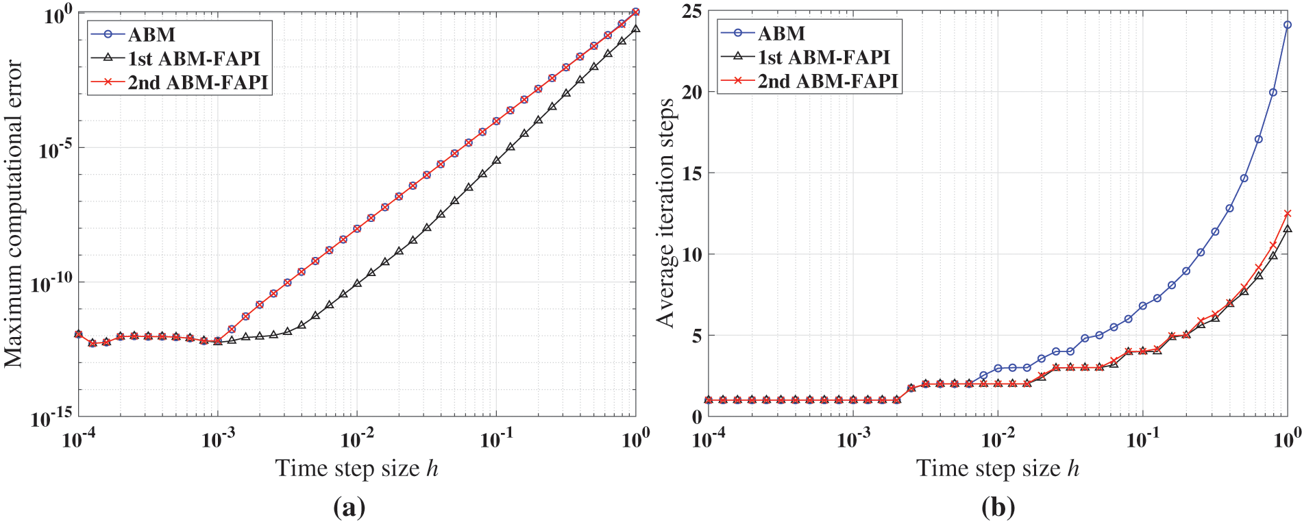
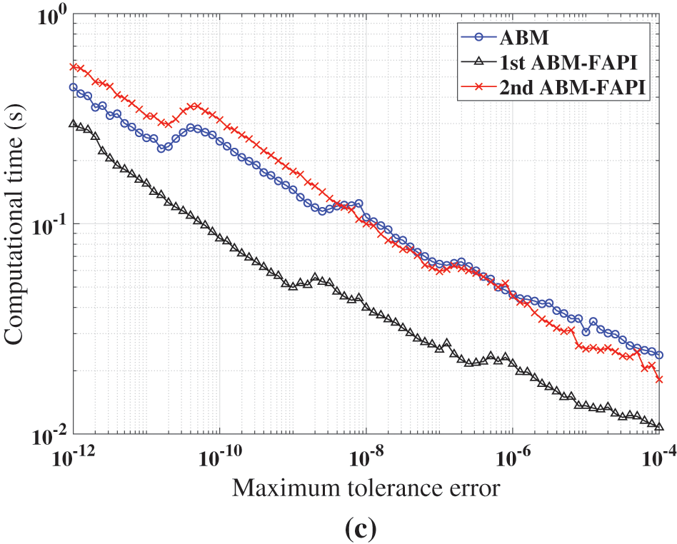
Figure 14: Performance of ABM, and ABM-FAPI in solving Mathieu equation when the algorithms converge: (a) Maximal error; (b) average iteration steps; (c) computational time
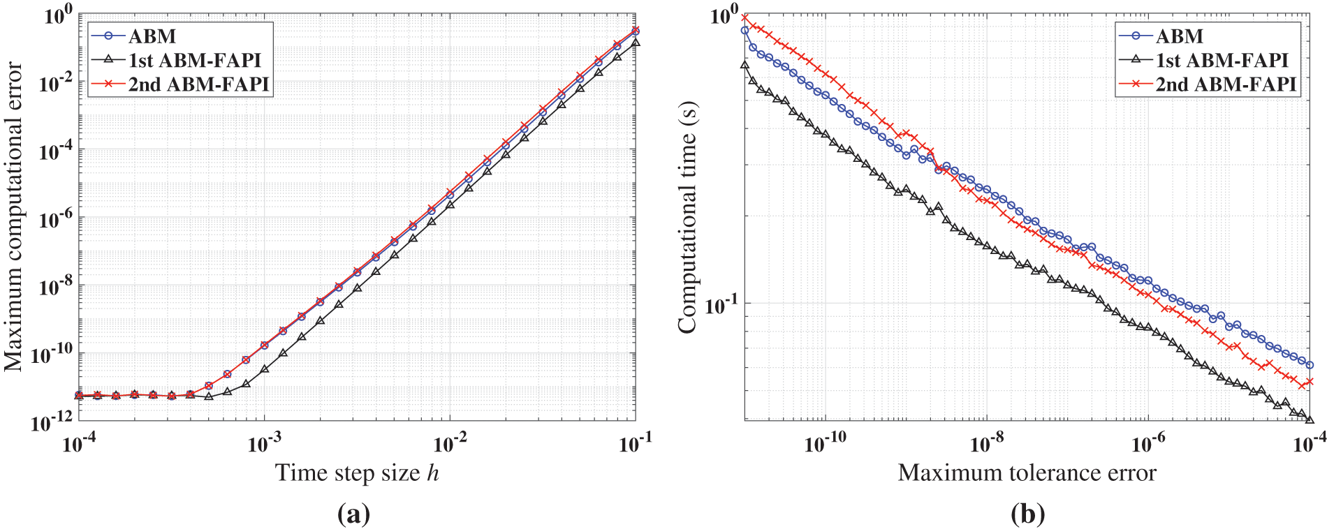
Figure 15: Performance of ABM, and ABM-FAPI in solving the forced Duffing equation when the algorithms converge: (a) Maximal error; (b) computational time
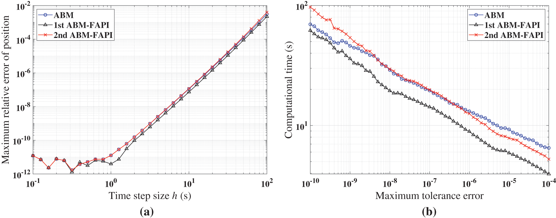
Figure 16: Performance of ABM, and ABM-FAPI for LEO when the algorithms converge: (a) Maximal error; (b) computational time
The simulation findings indicate that, in all cases, the 1st ABM-FAPI method significantly reduces computational time compared with the classical ABM method. For instance, as shown in Fig. 14c, the 1st ABM-FAPI method can save approximately
Fig. 14b demonstrates that the convergence speeds of the two versions of the ABM-FAPI method are almost the same. The ABM and ABM-FAPI methods converge at the same speed when the step size is small. However, the convergence speed of the ABM method lags behind that of the ABM-FAPI method as the step size increases.
Furthermore, the algorithm complexity of the 2nd ABM-FAPI method, which incorporates more information about the Jacobi matrix at time nodes, is significantly higher than that of the 1st ABM-FAPI method. However, as shown in Figs. 11–16, the performance of the 2nd ABM-FAPI method does not significantly outperform that of other methods, whereas the relatively “simpler” 1st ABM-FAPI method exhibits a significant advantage in computational accuracy and efficiency.
4.3 Implicit Runge-Kutta Method Using FAPI
The initial approximation in each step is selected as a straight line without additional computation of the derivatives when using the IRK method and the corresponding IRK-FAPI method to solve the nonlinear system. This initial approximation serves as a “cold start” for the methods. Generally, the “cold start” is a very rough prediction method.
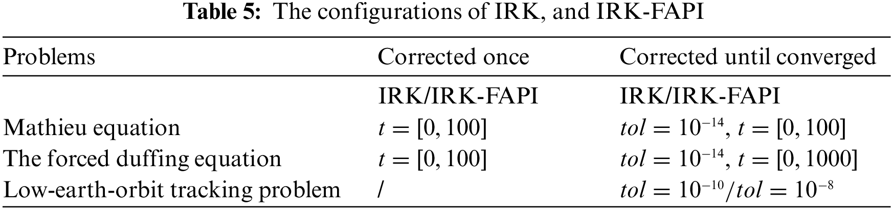
Figs. 17–19 show the simulation results when correcting once. Table 5 presents the duration of the simulated dynamical response. Due to the notably poor accuracy of the IRK method, to the extent that it can barely satisfy the corresponding accuracy requirements in some cases, its computational time is not recorded.
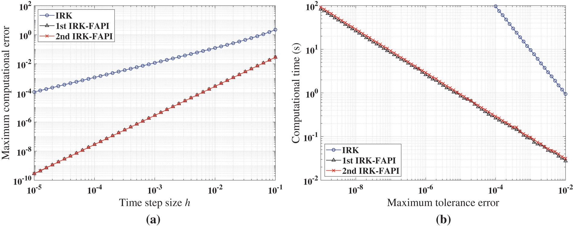
Figure 17: Performance of IRK, and IRK-FAPI in solving Mathieu equation when corrected only once: (a) Maximal error; (b) computational time
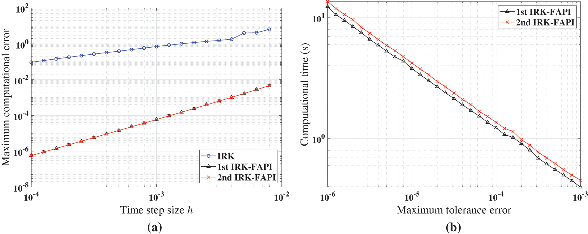
Figure 18: Performance of IRK, and IRK-FAPI in solving the forced Duffing equation when corrected only once: (a) Maximal error; (b) computational time
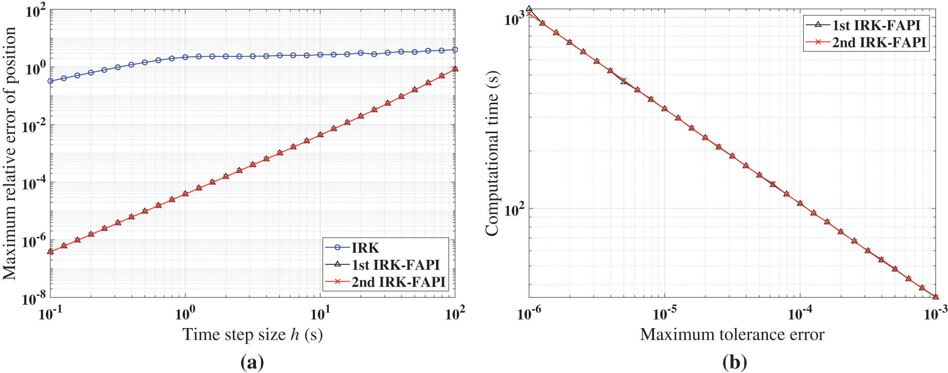
Figure 19: Performance of IRK, and IRK-FAPI for LEO when corrected only once: (a) Maximal error; (b) computational time
Figs. 17–19 demonstrate that the IRK-FAPI method outperforms the IRK method with extremely rough initial guesses in terms of accuracy and efficiency. As shown in Fig. 18, even with a very small step size, the IRK method cannot predict the long-term dynamical response of the chaotic system, whereas the IRK-FAPI method is very accurate by correcting once.
Similarly, Figs. 20–22 show the simulation results when the algorithm converges. Table 5 presents the configurations of these methods.
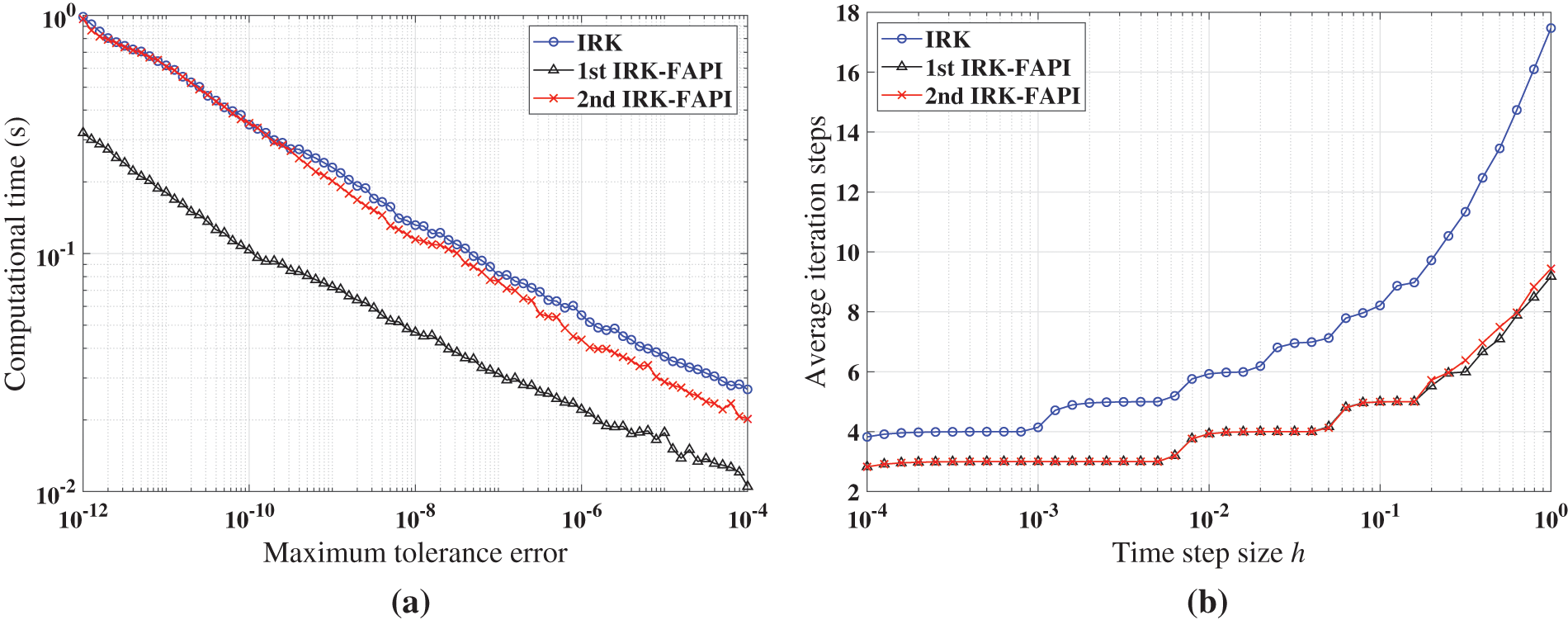
Figure 20: Performance of IRK, and IRK-FAPI in solving Mathieu equation when the algorithms converge: (a) computational time; (b) average iteration steps
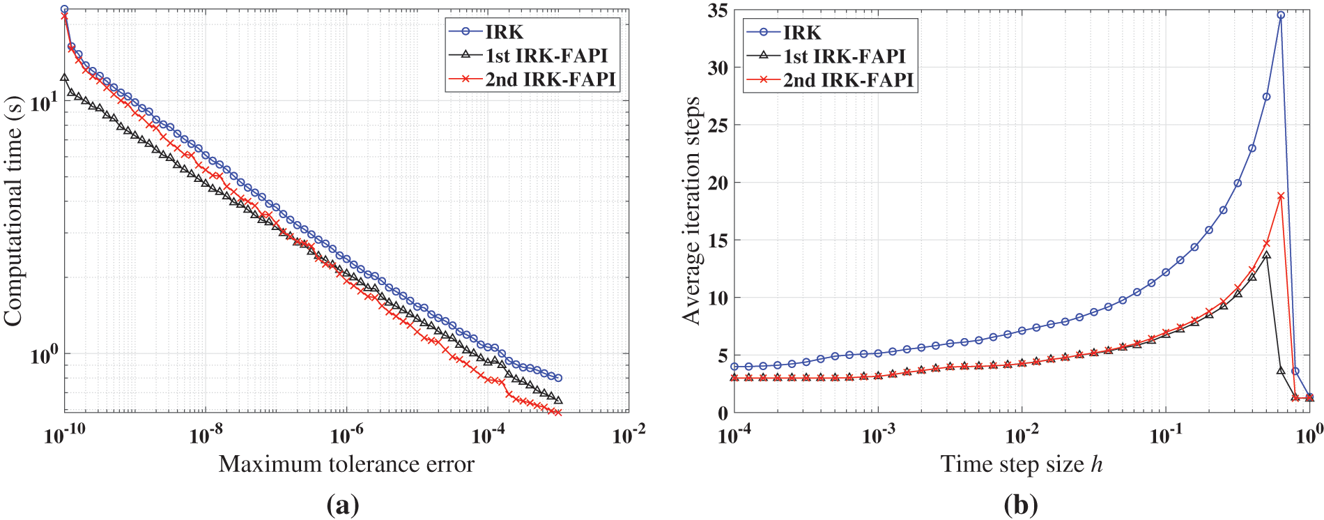
Figure 21: Performance of IRK, and IRK-FAPI in solving the forced Duffing equation when the algorithms converge: (a) computational time; (b) average iteration steps
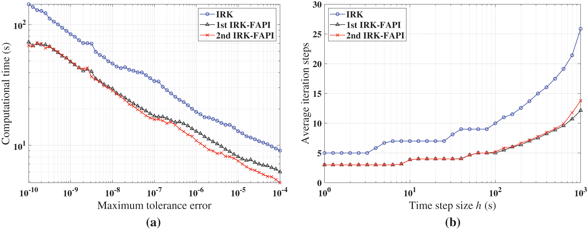
Figure 22: Performance of IRK, and IRK-FAPI for LEO when the algorithms converge: (a) computational time; (b) average iteration steps
Figs. 20–22 demonstrate that at least one of the two versions of the IRK-FAPI method will have higher computational efficiency than the IRK method, although the difference is not obvious in the case of the Duffing-Holmes’s oscillator. For instance, when solving the Mathieu equation, the 1st ABM-FAPI method can save more than half the computational time of the ABM method. Furthermore, the two versions of the IRK-FAPI method converge at almost the same speed, and both converge faster than the IRK method.
This study proposes a novel approach for deriving efficient predictor-corrector approaches based on FAPI. Three classical approaches, including the modified Euler approach, the Adams-Bashforth-Moulton approach, and the implicit Runge-Kutta approach, are used to demonstrate how FAPI can be employed to modify and improve commonly used predictor-corrector approaches. For each classical method, two versions of the FAPI correctors are derived. The resulting six FAPI-featured approaches are further used to numerically solve three different types of nonlinear dynamical systems originating from various research fields, ranging from mechanical vibration to astrodynamics. The numerical findings indicate that these enhanced correctors can effectively solve these problems with high accuracy and efficiency, with the 1st version of FAPI featured methods displaying superior performance in most cases. For instance, the 1st FAPI correctors achieve 1–2 orders of magnitude higher accuracy and efficiency than conventional correctors in solving the Mathieu equation. Furthermore, at least one version of the FAPI correctors shows superiority over the original correctors in all these problems, particularly when the correctors are used only once per step. In future studies, the application of the proposed approach to bifurcation problems and high-dimensional nonlinear structural problems will be presented.
The proposed approach offers a general framework for enhancing existing predictor-corrector methods by deriving new correctors using FAPI. Although three existing methods were retrofitted and their improvements demonstrated with three problems, it is anticipated that similar enhancements can be achieved by applying the proposed approach to various other predictor-corrector methods and nonlinear problems. For clarity, methods with low approximation orders (<5) were selected to illustrate our approach. However, methods of higher order can also be derived using the same procedure. In addition, our method can be directly combined with existing adaptive computational approaches for predictor-corrector methods to adaptively solve real-world problems.
Acknowledgement: The authors are grateful for the support by Northwestern Polytechnical University and Texas Tech University. Additionally, we would like to express our appreciation to anonymous reviewers and journal editors for assistance.
Funding Statement: This work is supported by the Fundamental Research Funds for the Central Universities (No. 3102019HTQD014) of Northwestern Polytechnical University, Funding of National Key Laboratory of Astronautical Flight Dynamics, and Young Talent Support Project of Shaanxi State.
Author Contributions: The authors confirm contribution to the paper as follows: study conception and design: Xuechuan Wang, Wei He; data collection: Wei He; analysis and interpretation of results: Xuechuan Wang, Wei He, Haoyang Feng; draft manuscript preparation: Xuechuan Wang, Wei He, Haoyang Feng, Satya N. Atluri. All authors reviewed the results and approved the final version of the manuscript.
Availability of Data and Materials: The data supporting the conclusions of this article are included within the article. Any queries regarding these data may be directed to the corresponding author.
Conflicts of Interest: The authors declare that they have no conflicts of interest to report regarding the present study.
References
1. Butcher, J. C. (2016). Numerical methods for ordinary differential equations. USA: John Wiley & Sons. [Google Scholar]
2. Smith, G. D., Smith, G. D., Smith, G. D. S. (1985). Numerical solution of partial differential equations: Finite difference methods. UK: Oxford university press. [Google Scholar]
3. Hilber, H. M., Hughes, T. J., Taylor, R. L. (1977). Improved numerical dissipation for time integration algorithms in structural dynamics. Earthquake Engineering & Structural Dynamics, 5(3), 283–292. [Google Scholar]
4. Fox, L. (1962). Numerical solution of ordinary and partial differential equations. UK: Pergamon Press. [Google Scholar]
5. Süli, E. (2010). Numerical solution of ordinary differential equations. UK: University of Oxford. [Google Scholar]
6. Meyer, K., Hall, G., Offin, D. (2008). Introduction to hamiltonian dynamical systems and the N-body problem. German: Springer Science and Business Media. [Google Scholar]
7. Turan, E., Speretta, S., Gill, E. (2022). Autonomous navigation for deep space small satellites: Scientific and technological advances. Acta Astronautica, 83, 56–74. [Google Scholar]
8. Xu, S., Peng, H. (2019). Design, analysis, and experiments of preview path tracking control for autonomous vehicles. IEEE Transactions on Intelligent Transportation Systems, 21(1), 48–58. [Google Scholar]
9. Wang, X., Yue, X., Dai, H., Atluri, S. N. (2017). Feedback-accelerated picard iteration for orbit propagation and lambert’s problem. Journal of Guidance, Control, and Dynamics, 40(10), 2442–2451. [Google Scholar]
10. Inokuti, M., Sekine, H., Mura, T. (1978). General use of the lagrange multiplier in nonlinear mathematical physics. Variational Method in the Mechanics of Solids, 33(5), 156–162. [Google Scholar]
11. Wang, X., Atluri, S. N. (2017). A novel class of highly efficient and accurate time-integrators in nonlinear computational mechanics. Computational Mechanics, 59, 861–876. [Google Scholar]
12. Wang, X., Xu, Q., Atluri, S. N. (2020). Combination of the variational iteration method and numerical algorithms for nonlinear problems. Applied Mathematical Modelling, 79, 243–259. [Google Scholar]
13. Atluri, S. N. (2005). Methods of computer modeling in engineering & the sciences, vol. 1. USA: Tech Science Press. [Google Scholar]
14. Plimpton, S. (1995). Fast parallel algorithms for short-range molecular dynamics. Journal of Computational Physics, 117(1), 1–19. [Google Scholar]
15. Noël, J. P., Kerschen, G. (2017). Nonlinear system identification in structural dynamics: 10 more years of progress. Mechanical Systems and Signal Processing, 83, 2–35. [Google Scholar]
16. Nazir, G., Zeb, A., Shah, K., Saeed, T., Khan, R. A. et al. (2021). Study of COVID-19 mathematical model of fractional order via modified euler method. Alexandria Engineering Journal, 60(6), 5287–5296. [Google Scholar]
17. Kumar, S., Kumar, R., Agarwal, R. P., Samet, B. (2020). A study of fractional lotka-volterra population model using haar wavelet and adams-bashforth-moulton methods. Mathematical Methods in the Applied Sciences, 43(8), 5564–5578. [Google Scholar]
18. Kennedy, C. A., Carpenter, M. H. (2019). Diagonally implicit runge–kutta methods for stiff odes. Applied Numerical Mathematics, 146, 221–244. [Google Scholar]
19. Kovacic, I., Rand, R., Mohamed Sah, S. (2018). Mathieu’s equation and its generalizations: Overview of stability charts and their features. Applied Mechanics Reviews, 70(2), 020802. [Google Scholar]
20. Singh, H., Srivastava, H. (2020). Numerical investigation of the fractional-order liénard and duffing equations arising in oscillating circuit theory. Frontiers in Physics, 8, 120. [Google Scholar]
21. Amato, D., Bombardelli, C., Baù, G., Morand, V., Rosengren, A. J. (2019). Non-averaged regularized formulations as an alternative to semi-analytical orbit propagation methods. Celestial Mechanics and Dynamical Astronomy, 131(5), 1–38. [Google Scholar]
22. Zennaro, M. (1986). Natural continuous extensions of runge-kutta methods. Mathematics of Computation, 46(173), 119–133. [Google Scholar]
Cite This Article
 Copyright © 2024 The Author(s). Published by Tech Science Press.
This work is licensed under a Creative Commons Attribution 4.0 International License , which permits unrestricted use, distribution, and reproduction in any medium, provided the original work is properly cited.
 Downloads
 Citation Tools