An Efficient Reliability-Based Optimization Method Utilizing High-Dimensional Model Representation and Weight-Point Estimation Method

1  Introduction

Many uncertainty factors inevitably exist in practical engineering problems and affect the performance of structural systems to some extent [1–3]. Therefore, it is critical to consider the uncertain influence of structural systems on reliability-based design optimization (RBDO) [4,5]. RBDO produce more reliable design results compared to those obtained using traditional deterministic optimization methods [6,7]. Existing RBDO methods can be roughly divided into three categories: the nested double-loop method (NDLM), single loop method (SLM), and decoupled-loop method (DLM).

NDLM is the original RBDO method and is executed with alternating inner and outer layer calculations. The outer layer performs deterministic optimization analysis for the design variables and the inner layer performs probabilistic analysis for the reliability constraints [8]. Because the inner-layer probability analysis requires a large number of computations and each outer-layer optimization iteration must invoke inner-layer probability analysis, the efficiency of RBDO based on NDLM is relatively low. Regardless, this method can be considered as a milestone in RBDO and has received extensive attention in the field of structural system design [9].

Efficient algorithms such as SLM and DLM have emerged to improve the computational efficiency of RBDO. For SLM, the processes of searching for optimal design variables and calculating the most probable failure points occur simultaneously. This process overcomes the drawbacks of NDLM to some extent and has been widely applied in practical engineering problems. Wang et al. [10] proposed a non-probabilistic reliability-based optimization method based on SLM and applied it to the optimization of a supersonic wing. Their method uses first-order interval Taylor expansion, the interval vertex theorem, and direct optimization methods to analyze the uncertainty propagation problem of a system. Additionally, the extended non-probabilistic set theory-stress strength interference model and volume ratio theory are introduced to evaluate the non-probabilistic index reasonably. Jiang et al. [11] proposed an adaptive hybrid single-loop method (AH-SLM). An iterative control strategy (ICS) with two iterative control criteria is proposed. This strategy converges rapidly, regardless of the degree of non-linearity of the performance function, and improves the accuracy of the most probable point (MPP) in highly nonlinear problems. Keshtegar et al. [12] proposed a novel RBDO based on SLM and applied it to the design of aircraft stiffened plates with complex bucking constraints. The results demonstrated that their method has enhanced computational efficiency and robustness. Additional studies on SLM include references [13–15]. One can see that SLM is not only suitable for probabilistic RBDO, but also provides a good performance for non-probabilistic RBDO. Currently, the research on this method mainly focuses on handling highly nonlinear probabilistic constraints and rapid convergence. To reduce the computational burden further, the RBDO of complex structure systems through the combination of surrogate models and SLM is an emerging trend [16].

DLM first transforms reliability constraints into general deterministic constraints. Converted RBDO problems can then be solved utilizing traditional deterministic optimization methods. In [17,18], it is replaced the MPP with a quantile-based decoupling method to overcome the drawbacks of the original method that requires solving the MPP. This is particularly important for highly nonlinear problems, multiple-MPPs and non-normally distributed variables. In this approach, quantitative metrics are obtained by sampling a surrogate model and a new sample is selected using a sample-updating strategy in the significant region [19,20]. Overall, this method yields good performance for complex structures. Shi et al. [21] utilized a two-step method to implement a novel form of decoupling. Because this method involves only a small amount of time-varying reliability analysis and deterministic optimization, the efficiency of time-varying reliability optimization is improved to some extent. Zhang et al. [22] used a Kriging surrogate model [23,24] to handle RBDO problems with independent constraint functions and then proposed a novel quantile-based sequential RBDO approach. In this method, an adaptive Kriging scheme with error control is integrated to derive the accuracy information of the surrogate model. The proposed independent training strategy reduces the number of function evaluations while maintaining the accuracy of reliability estimation. Other studies on DLM include references [25,26]. Most DLM implementations are similar to SLM. However, there is no method for completely decoupling the reliability of the inner layer and optimization analysis of the outer layer because it is difficult to determine the functional relationships between reliability constraints and design variables directly.

In this study, a fully decoupled RBDO method is developed by combining high dimensional model representation (HDMR) [27] and the weight point estimation method (WPEM) [28]. First, the reliability constraint function is decomposed using HDMR and then combined with WPEM and the first-order reliability method (FORM) [29] to decompose the reliability index into a combination of a series of univariate functions. Second, the univariate function is fitted using Lagrange interpolation [30]. Finally, a traditional deterministic optimization method is utilized to obtain optimal design variables.

The remainder of this paper is organized as follows. Section 2 briefly introduces the basic principles of RBDO and HDMR. Section 3 presents the derivation of the reliability index based on HDMR and WPEM. The proposed decoupled RBDO model is detailed in Section 4. In Section 5, two numerical examples of a planar 10-bar structure and an aviation hydraulic piping system (AHPS) with 28 design variables involving finite element analysis are presented to illustrate the performance and practicality of the proposed method. Finally, our conclusions are summarized in Section 6.

2  Brief Review of RBDO and HDMR

2.1 Reliability-Based Design Optimization

The goal of RBDO is to derive optimal design variables that meet the reliability requirements of an engineering system. Generally, RBDO is mathematically expressed as follows:

minimize f(d)subject to Rk=Pr(gk(x,d)≤εk)≥=Rkta,  k=1,…,NcdiL≤di≤diU,  i=1,…,Nd(1)

where x=(x1,x2,…,xn)T and d=(d1,d2,…,dm)T are the random parameter and design variable, respectively, and n and m are the numbers of random parameters and design variables, respectively. f is the objective function, and Rk, gk, εk and Rkta are the reliability, performance function, security threshold and target reliability levels of the kth reliability constraint, respectively. Nc is the number of reliability constraints, diL and diU are the lower and upper bounds of the ith design variable di, respectively, and Nd is the number of design variables.

2.2 High Dimensional Model Representation

Two types of HDMR are commonly used in the reliability field, namely the multiplication dimension reduction method (MDRM) [31] and conventional dimension reduction method (CDRM) [32]. In this study, MDRM is utilized to handle reliability constraints and it is formulated as follows:

g(x)=g(xc)(1−n)∏i=1ngi(x−ic)(2)

where xc=(x1c,x2c,…,xnc) represents a specific reference vector of a random vector. For a random variable that follows a normal distribution, its reference point is generally regarded as its mean value. x−ic=(x1c,x2c,…,xi−1c,xi,xi+1c,…,xnc) denotes the reference points other than xi and gi is the univariate function of xi.

3  Reliability Index Based on MDRM and WPEM

Because the relationship between the reliability level and reliability index is R=Φ(β), the reliability constraint in Eq. (1) can be transformed into

βk≥βkta,  k=1,…,Nc(3)

where Φ is the cumulative distribution function, and βk and βkta are the reliability indices of the ith event gk(x,d)≤εk and kth target reliability index, respectively. Then, Eq. (1) can be rewritten as

minimize f(d)subject to βk≥βkta,  k=1,…,NcdiL≤di≤diU,i=1,…,Nd(4)

Many methods can be used to calculate β, including FORM [27] and the second-order reliability method [33]. Because FORM is most commonly used in actual engineering structural reliability analysis, we used FORM to calculate β, which is expressed as

β=ε−μgσg(5)

where μg, σg and ε denote the mean and standard deviations of the performance function and security threshold, respectively.

According to MDRM, as shown in Eq. (2), a performance function containing both random and design variables can be decomposed into the following form in a similar manner:

g(x,d)=g(xc,dc)(1−n−m)∏i=1ngi(x−ic,dc)∏j=1mgj(xc,d−jc)(6)

where gj denotes the univariate function of the jth design variable dj and dc=(d1c,d2c,…,dmc) represents the reference vector of the design vector, which can be considered as the most valuable point among the design variables. In this study, the central point of the design variables is considered as the reference point. d−jc denotes the reference vector, excluding dj. The performance function is decomposed into two parts using Eq. (6), where one is the product of the random univariate functions gi(x−ic,dc) and the other is the product of the design univariate function gj(xc,d−jc).

Next, the relationship between the reliability index β and design variables d is deduced based on Eq. (6). The deduction process for the mean μg and variance σg2 is as follows:

μg=E[g(x,d)]=g(xc,dc)1−n−m∏j=1mgj(xc,d−jc)∏i=1n∫gi(x−ic,dc)f(xi)dxi=ξ∏j=1mgj(xc,d−jc)(7)

σg2=E[g(x,d)2]−(E[g(x,d)])2=g(xc,dc)2(1−n−m)(∏j=1mgj(xc,d−jc))2∏i=1n∫gi(x−ic,dc)2f(xi)dxi−(μg)2=g(xc,dc)2(1−n−m)(∏i=1n∫gi(x−ic,dc)2f(xi)dxi−(∏i=1n∫gi(x−ic,dc)f(xi)dxi)2)×(∏j=1mgj(xc,d−jc))2=ζ2(∏j=1mgj(xc,d−jc))2(8)

where ξ and ζ are expressed as follows:

ξ=g(xc,dc)1−n−m∏i=1n∫gi(x−ic,dc)f(xi)dxi(9)

ζ=g(xc,dc)(1−n−m)(∏i=1n∫gi(x−ic,dc)2f(xi)dxi−(∏i=1n∫gi(x−ic,dc)f(xi)dxi)2)(10)

In Eqs. (7)–(10), f(xi) denotes the cumulative distribution function of the xi. ∫gi(x−ic,dc)f(xi)dxi and ∫gi(x−ic,dc)2f(xi)dxi are the first and second origin moments of gi(x−ic,dc), respectively. If the distribution type and parameters of xi are known in advance, then the two moments can be calculated through a series of WPEM applications (e.g., sparse grid integration [34], seven-point estimation (a Gauss quadrature method), or three-point estimation [27]). Therefore, ξ and ζ are constants. In this study, a three-point estimation is adopted to solve the first- and second-order origin moments, as detailed below.

According to the principles of WPEM, the first and second moments of gi(x−ic,dc) can be approximated as

Mgi1=∫gi(x−ic,dc)f(xi)dxi≈∑j=1kwijgi(pij,x−ic,dc)(11)

Mgi2=∫gi(x−ic,dc)2f(xi)dxi≈∑i=1kwijgi(pij,x−ic,dc)2(12)

where f(xi) is the probability density function of xi, and wij and pij are the weight and feature points corresponding to xi, respectively. k denotes the number of weight points.

In Eqs. (11) and (12), one can see that if wij and pij are known in advance, then Mgi1 and Mgi2 can be solved using WPEM. wij and pij in the three-point estimation approach can be calculated using the following equations:

wi1=12(1+λ3xi/4λ4xi−3λ3xi2λ4xi−λ3xi2)(13)

wi2=1−1λ4xi−λ3xi2(14)

wi3=12(1−λ3xi/4λ4xi−3λ3xi2λ4xi−λ3xi2)(15)

pi1=λ1xi−λ2xi2(4λ4xi−3λ3xi2−λ3xi)(16)

pi2=λ1xi(17)

pi3=λ1xi+λ2xi2(4λ4xi−3λ3xi2+λ3xi)(18)

where λ1xi, λ2xi, λ3xi and λ4xi denote the first four moments of xi. The first four moments are the mean, standard deviation, kurtosis and skewness in order. The corresponding standard normally distributed variables are zero, one, zero and three in order.

By combining Eq. (5) with Eq. (7) to Eq. (10), the reliability index β can be rewritten as

β=ε−ξ∏j=1mgj(xc,d−jc)ζ∏j=1mgj(xc,d−jc)(19)

As shown in Eq. (19), β is only a function of the design variables and is independent of the random variables.

4  Decoupled RBDO Model

According to the basic principles described in the previous section, two types of decoupled RBDO models can be formulated. In the first RBDO model, the reliability level is given by R=Pr(g(x,d)≤ε) and the corresponding reliability constraint can be deduced as follows:

ε−ξ∏j=1mgj(xc,d−jc)ζ∏j=1mgj(xc,d−jc)≥βta⇔C∏j=1mgj(xc,d−jc)−ε≤0(20)

where C=(ζβta+ξ) is a constant. Furthermore, the RBDO model can be decoupled into the following deterministic optimization model:

minimize f(d)subject to Ck∏j=1mgjk(xc,d−jc)−εk≤0,  k=1,…,NcdiL≤di≤diU,  i=1,…,Nd(21)

In the second RBDO model, the reliability level is expressed as R=Pr(g(x,d)≥ε). Therefore, the reliability index can be rewritten as follows:

β=ξ∏j=1mgj(xc,d−jc)−εζ∏j=1mgj(xc,d−jc)(22)

Then, the reliability constraint can be deduced in the following form:

ξ∏j=1mgj(xc,d−jc)−εζ∏j=1mgj(xc,d−jc)≥βta⇔ε−C′∏j=1mgj(xc,d−jc)≤0(23)

where C′=(ξ−ζβta) is a constant. Furthermore, the corresponding decoupled RBDO model is expressed as follows:

minimize f(d)subject to εk−Ck′∏j=1mgjk(xc,d−jc)k≤0,k=1,…,NcdiL≤di≤diU,  i=1,…,Nd(24)

The optimization models defined in Eqs. (21) and (24) are deterministic optimization models with respect to the design variables that can be solved using any traditional optimization algorithm. In this study, Monte Carlo simulation (MCS), sequential quadratic programming (SQP) [35] and particle swarm optimization (PSO) [36] we adopted to verify the performance of the proposed method.

Eqs. (21) or (24) can be used directly to solve the RBDO model when the constraint is an explicit function, whereas for an RBDO model with an implicit constraint function, Lagrange interpolation is adopted to fit the univariate function gjk(xc,d−jc) as follows:

L(x)=∑k=1Nlykϕk(x)(25)

where

ϕk(x)=∏j=1j≠kNlx−xjxk−xj(26)

In Eqs. (25) and (26), Nl denotes the number of samples, xj denotes the jth input sample, and yk denotes the kth output sample. In this study, the input samples are evenly distributed within the design interval. A flowchart of the proposed RBDO algorithm is presented In Fig. 1.

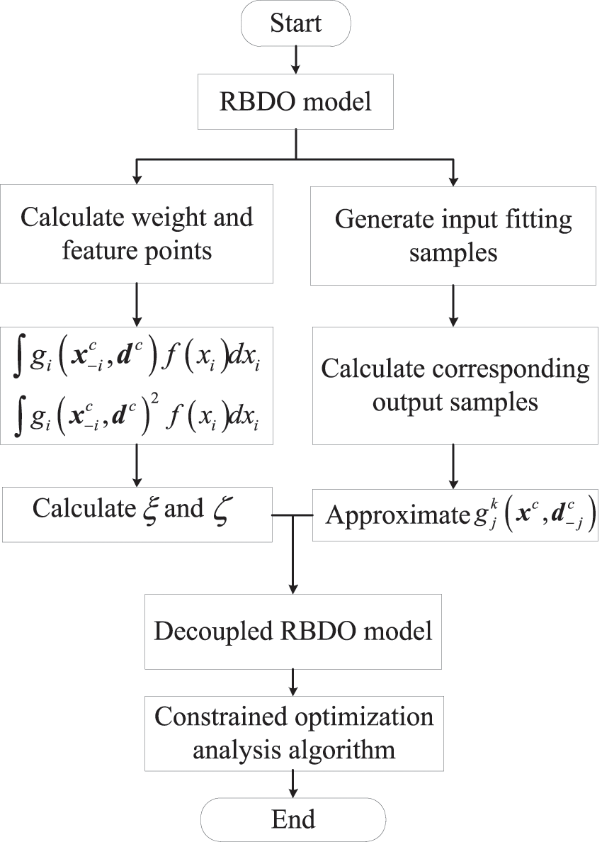
Figure 1: Flowchart of the proposed RBDO algorithm

As shown in Fig. 1, the calculation steps of the proposed method can be divided into two main parts. The first is calculating two constants ξ and ζ for the random variables and the second is fitting the univariate function gjk(xc,d−jc) using Lagrange interpolation. Therefore, the computational cost of the proposed approach depends on these two operations. Assuming that the numbers of random variables, design variables, and constraint functions are n, m and k, respectively, and that there are p input samples in each design variable, the number of function evaluations in the proposed method is 3 × n + (p × m) × k. For example, when n, m, k and p are 2, 2, 2 and 4, respectively, the number of function evaluations for RBDO analysis is 22, which demonstrates that the proposed approach is relatively efficient.

Notably, the application of the proposed method must focus on the following two points.

(1) The premise of applying the proposed method is assumption that the performance function of all constraints is greater than 0. Otherwise, the performance functions in the reliability constraint must be transformed to ensure that they are greater than 0. For example, suppose that the performance function in R=Pr(g(x,d)≤ε) is less than 0, i.e., g(x,d)≤0. Then, there is a non-negative constant γ that makes Eq. (27) true.

g′(x,d)=g(x,d)+γ≤0+γ(27)

In Eq. (27), the value of γ should be sufficiently large to ensure that g′(x,d)=g(x,d)+γ>0, g′(x,d) is the corresponding new performance function, which must be greater than 0. Assume that ε′=ε+γ is the corresponding new threshold. Then, R′=Pr(g′(x,d)≤ε′) is the corresponding new reliability level and R′=R. Finally, the reliability constraint is transformed as follows:

R′=Pr(g′(x,d)≤ε′)≥=Rta(28)

(2) According to Wang et al. [10], there are three combination types between the design variable d and random variable x. The first type is direct mixing of the design variable and random variable (i.e., (d,x)). The second type is that the design variable is a parameter of the random variable (e.g., such as x∼N(d,σ)). The third type contains both the first type and second type. However, any of these types can be transformed into the first type by the following formula:

U=x−dσ⇒x=d+Uσ(29)

where U∼N(0,1). Therefore, only the first combination type is considered in this study.

5  Illustrative Examples

In this section, two numerical examples of a planar 10-bar structure and AHPS that requires finite element software calculations are presented to illustrate the performance of the proposed method. The proposed method is set up to use SQP and PSO (abbreviated as PM-SQP and PM-PSO, respectively) to perform the optimization analysis, and the results of direct MCS (MCS-D) and a combination of MCS and PSO (MCS-PSO) are used as references. It is noteworthy that MCS-D is a direct MCS method that has the greatest reference value. However, because the optimization module is still MCS, there may be some errors. Therefore, using PSO can further ensure the correctness of the reference results (MCS-PSO). PM-SQP and PM-PSO are implemented based on the proposed method with Lagrange interpolation proxy models after complete decoupling. The difference between these models lies in the optimization methods, which are only used to verify the accuracy of the models.

5.1 Numerical Example 1

A numerical example with two design variables (d1,d2) and two random variables (x1∼N(0,1), x2∼N(0,1)) is defined in Eq. (30). The target reliability of Rta is set to 0.9987 with d1∈[2,5], d2∈[2,5], and ε=1.

minimize f(d)=(d1+d2)/2subject to R=Pr(g≥ε)≥Φ(βta)=Rtag=(d1+0.3x1)2(d2+0.3x2)/202≤d1,d2≤5(30)

The samples required to approximate the input-output relationship of the univariate function using Eqs. (25) and (26) are defined as dsamples1=dsamples2=(2,3,4,5). Given 105 samples for MCS, the optimization results are presented in Table 1.

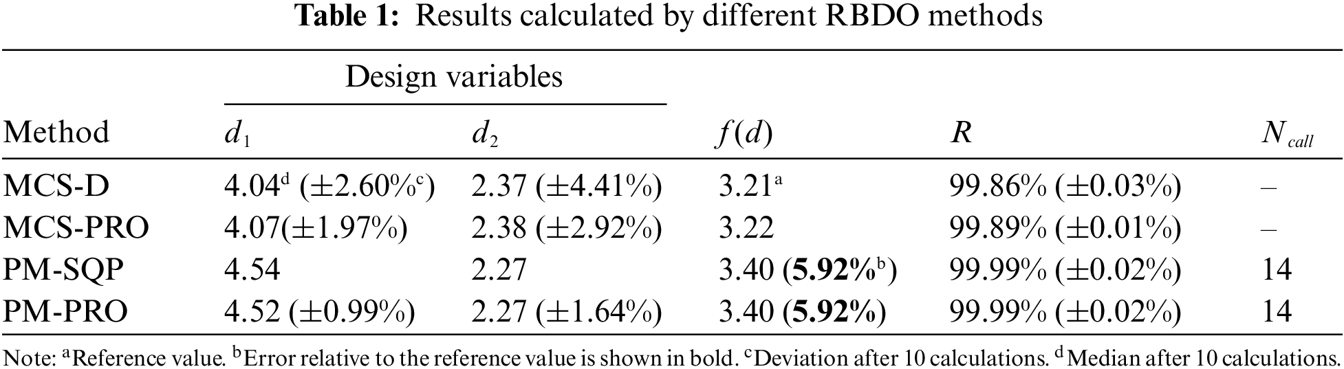
The reliability level R in Table 1 is calculated by applying MCS 10 times and the design variable values are the corresponding median values. The reliability level obtained by MCS-D is 99.86%, which is lower than the target reliability level of 99.87%. This is because the optimal design variables obtained by MCS-D are the optimal solutions based on 105 samples, so the median value of 10 calculations is generally less than the target reliability level and it is reasonable to use the optimal objective function value f(d) obtained by MCS-D as a reference. For MCS-PRO, the inner layer uses MCS for reliability analysis, and the outer layer uses PRO for optimization analysis. The results obtained by MCS-PRO can be used as an auxiliary reference, because the error of MCS-D is relatively large when the number of design variables is large or the sample size is limited.

In Table 1, one can see that the f(d) values calculated by PM-SQP and PM-PRO are the same at 3.40, which is slightly larger than the reference value of 3.22 calculated by MCS-PRO. The error of the proposed method is approximately 5.92%. The reliability level corresponding to the optimal design variables obtained by PM-SQP and PM-PRO is the same and equal to 99.99%, which is slightly higher than the target reliability level of 99.87%.

The relationship between the number of samples and the minimum value of f(d) is presented in Fig. 2. One can see that the value of f(d) remains largely unchanged after 3 samples and 4 samples can meet the accuracy requirement. The number of function calls Ncall is 14 for the proposed method, demonstrating that the computational efficiency of the proposed method is relatively high.

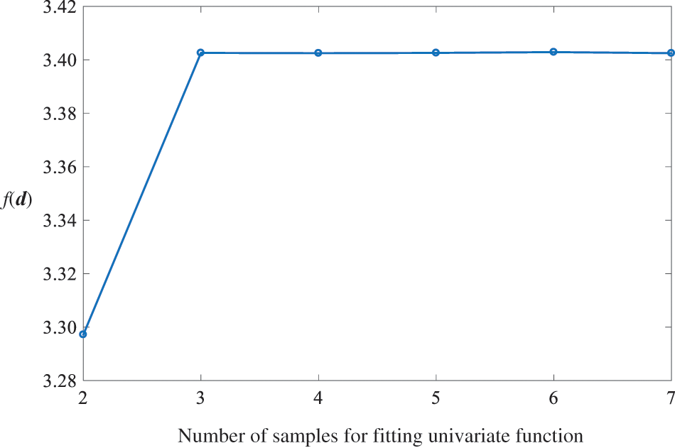
Figure 2: Objective function value changes with the number of samples

5.2 Numerical Example 2

A numerical example with four constraints that has been widely used for benchmarking purposes in previous studies [37,38] is defined in Eq. (31). Two random variables are normally distributed as x1∼N(d1,0.32) and x2∼N(d1,0.32), and d1 and d2 are two design variables with the same design range of [2,5]. The target reliability Rta is set to 0.9987 and four thresholds are assigned as ε1=ε2=ε3=ε4=1. Given an the input sample dsamples1=dsamples2=(2,3,4,5), the optimization results are presented in Table 2.

minimize f(d)=d1+d2subject to Rk=Pr(εk−gk(x,d)≤0)≥Φ(βkta)=Rta,  k=1,2,3,42≤d1,d2≤5g1=x12x2/20;g2=(x1+x2−5)2/30−(x1−x2−12)2/120;g3=80/(x12+8x2+5);g4=80/(x12+9x2+4);(31)

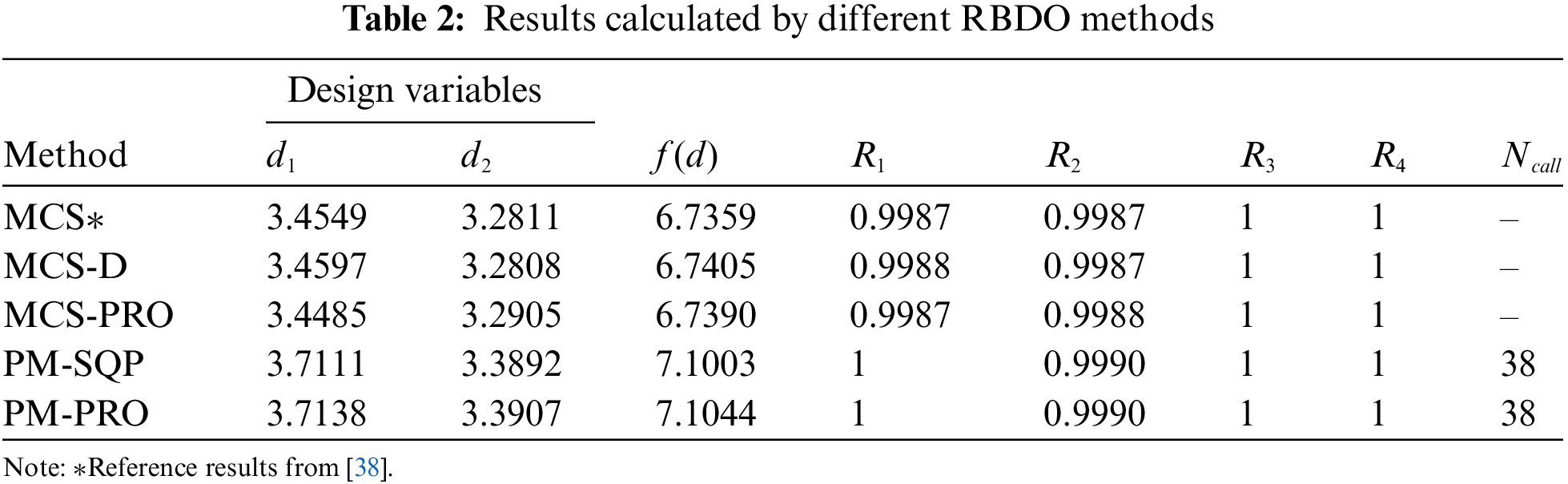
The results in Table 2 are obtained by executing each method once. The MCS results from [38] are presented to verify the correctness of the reference method. The results obtained by MCS and MCS-D are similar, indicating that it is reasonable to use the results of MCS-D as a reference. The minimum values obtained by PM-SQP and PM-PRO are very similar and the error is approximately 5.34% relative to the results obtained by MCS-D.

As shown in Fig. 3, because the objective function value is unchanged after 3 samples, 4 samples can meet the fitting accuracy requirement. The number of function evaluations for the proposed method is 38, indicating that the efficiency of the proposed method is relatively high.

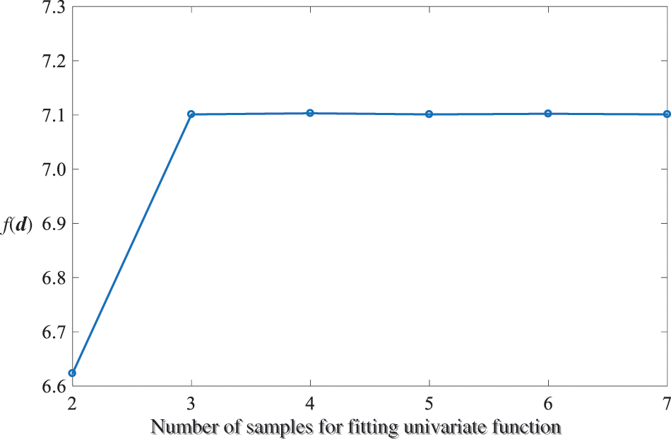
Figure 3: Objective function value changes with the number of samples

The two numerical examples demonstrate that the accuracy and efficiency of the proposed method are within acceptable ranges. Its accuracy depends on the accuracy of the formula used to calculate the reliability index. In this study, the first-order reliability method, which is the most widely used in practical engineering, resulting in a conservative calculation error of approximately 5%. Additionally, its computational efficiency depends entirely on the number of feature points in WPEM and the number of sample points fitting the univariate function, which are unrelated to subsequent optimization. Next, we apply the proposed method to two practical engineering problems using finite element software to demonstrate the feasibility of the proposed method for practical engineering problems.

5.3 Planar 10-Bar Structure

The plane 10-bar structure is presented in Fig. 4. The length of the rods is L, and the corresponding cross-sectional area is Ai(i=1,2,…,10), and the elasticity modulus and three external loads are E and Pi(i=1,2,3), respectively. L and Ai(i=1,2,…,10) are the 11 design variables, and E and Pi(i=1,2,3) are 4 random variables that follow normal distribution. An optimization model aimed at minimizing the volume of the 10-bar structure is established and expressed by Eq. (32).

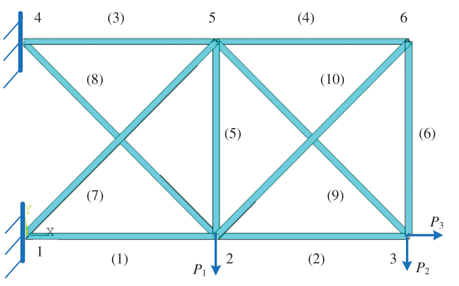
Figure 4: Planar 10-bar structure

minimize f(d)=d1(∑i=27di+2∑i=811di)subject to R=Pr(g(x,d)−ε≤0)≥Rtadil≤di≤diu(32)

where x=[x1,x2,x3,x4]=[E,P1,P2,P3], and the mean μ and standard deviation σ are listed in Table 3. Additionally, d=[d1,d2,…,d11]=[L,A1,A2,…,A10], g(x,d) is the maximum displacement response, dil and diu represents the lower and upper bounds of di, respectively, and the corresponding values are listed in Table 3.

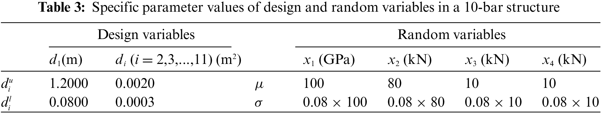
Given the threshold ε=0.0035(m) and target reliability level Rta=0.999, the optimization process and results are presented in Fig. 5 and Table 4, respectively.

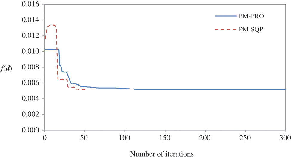
Figure 5: Optimization process of a planar 10-bar structure

Because PRO is a heuristic global optimization algorithm that is more suitable for the optimization of complex problems, only utilized PM-PRO to optimize the planar 10-bar structure. The finite element analysis model of the planar 10-bar structure is presented in Fig. 6, where the design variables are fixed at d1=1 and di(i=2,…,11)=0.001, and the maximum displacement is 0.0027 (m). It is noteworthy that this example required the use of the ANSYS commercial software and it would be a laborious process to calculate the reliability level using MCS. Therefore, the reliability levels listed in Table 4 are obtained by substituting the optimal design variables into Eq. (21).

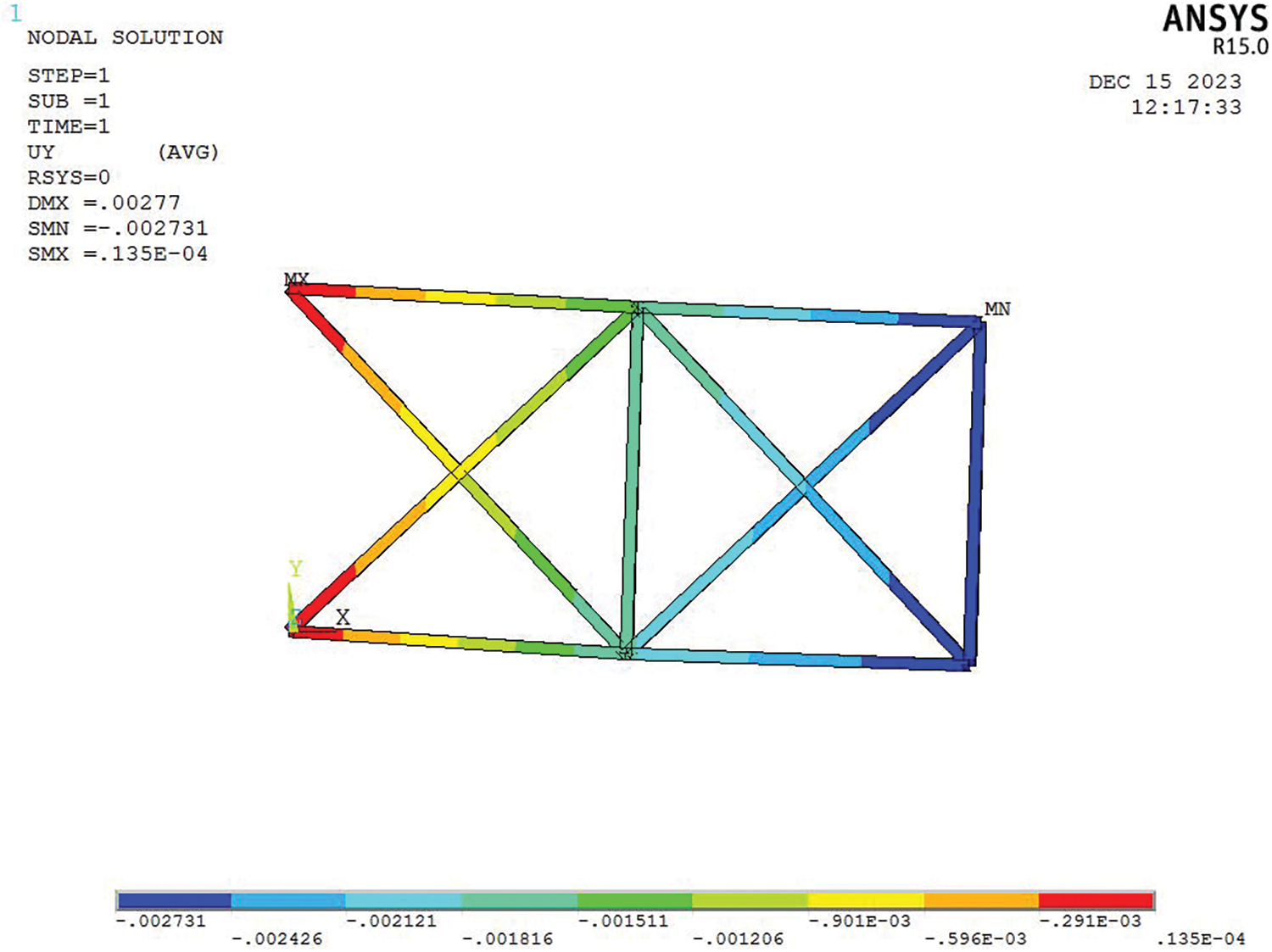
Figure 6: Displacement contour plot before optimization

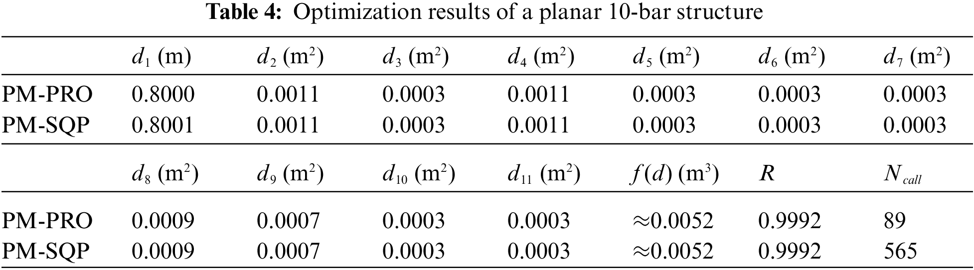
For this engineering optimization problem with 11 design variables, Fig. 7 reveals that the objective function value remained essentially unchanged after 6 sample points. Therefore, 7 samples are taken for each design variable to satisfy the basic accuracy requirements and only 89 function calls are required to solve the optimization problem. For an optimization model with 11 design variables and 4 random variables, the proposed method is relatively efficient. The FE model corresponding to the optimal solution of PM-SQP proposed in Table 4 is presented in Fig. 8.

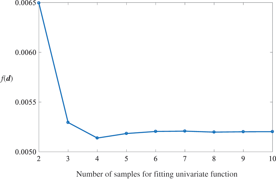
Figure 7: Objective function value changes with the number of samples

Figure 8: Displacement contour plot after optimization

5.4 Reliability Optimization of the Clamp Support Position in an AHPS

An AHPS is required for most aircraft operations and is one of the most critical aircraft accessories. Considering the long span of an AHPS, a large number of clamp supports are typically required to fix it and reduce the instability caused by engine vibration and fuselage flutter. A series of AHPS clamp support positions are presented in Fig. 9, while Fig. 10 presents the corresponding right-side view.

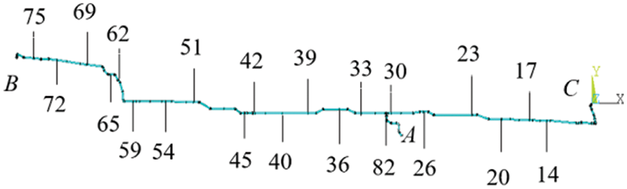
Figure 9: AHPS clamp support positions

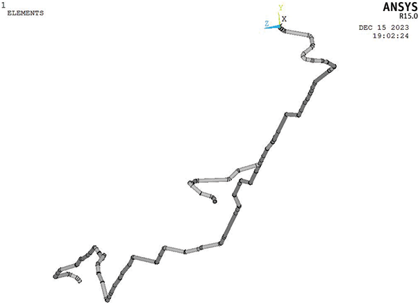
Figure 10: Right-side view of an AHPS

In Fig. 9, A is the pump source, and B and C are the two oil outlets. The numbers in Fig. 9 corresponding to nodes in the finite-element model, which are also the clamp support positions. The corresponding coordinates are listed in Table 5. The bold coordinates represent the initial values of the design variables and the superscripts are the corresponding serial numbers of the design variables (total of 28 design variables). As shown in Table 5, the design variables are the coordinates of the clamp position nodes and most of the design variables are X coordinates (e.g., nodes 14, 17, and 51). Some of the design variables are the X and Y coordinates of the corresponding notes (e.g., nodes 45, 62 and 69) and there are three design variables for nodes 82 representing X, Y, and Z coordinates.

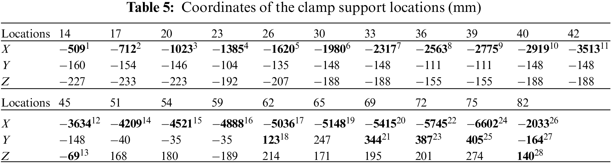
It is noteworthy that the coordinates in Table 5 are global coordinates, and the pipeline is modeled using the PIPE 16 unite in ANSYS. Considering the characteristics of the PIPE 16 unit, the pipeline is constructed using local coordinate, where the last node of each segment corresponded to the start of the next segment. Fig. 11 illustrates this type of construction for node 14 in Fig. 10.

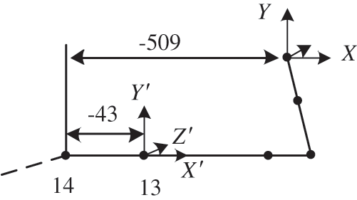
Figure 11: Illustration of PIPE16 unit modeling

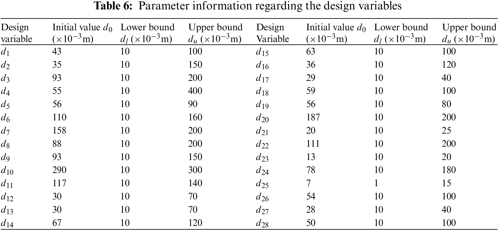
In Fig. 11, one can see that the global coordinate in the X direction of node 14 is −509, which corresponds to the value for node 14 listed in Table 5. The establishment of this section of the pipeline between nodes 13 and 14 begins at node 13 and the local coordinate in X direction is −43. For convenience, only local coordinates are used to describe the initial values d0, lower bounds dl and upper bounds du of the design variables, as shown in Table 6. The choice of upper and lower bounds for the design variables followed the principle that the shape of the pipeline cannot change when the design variables vary between the upper and lower bounds. Furthermore, the shape of the pipeline does changes whenever if a variable exceeds the upper or lower bounds. Therefore, the range of variable changes in Table 6 is optimal.

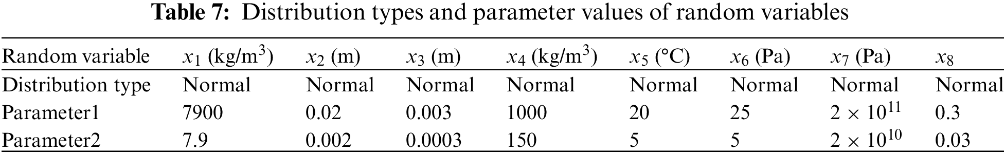
The random variables for the AHPS are the pipeline material density ρp, pipeline outer radius D, pipeline wall thickness t, fluid density ρf, ambient temperature T, oil pressure P, elastic modulus E, and Poisson’s ratio μ. For simplicity, we let x=[x1,x2,…,x8]=[ρp,D,t,ρf,T,P,E,μ]. The specific values of these variables are listed in Table 7 and additional values can be found in [39].

The random excitation applied to all clamp supports is an acceleration power spectral density function, as shown in Fig. 12 [39]. The scaling factor of excitation applied at the three endpoints of the AHPS (i.e., A, B, C) is 1, and 0.025 is applied at the other clamp supports. Because the excitation exerted on an AHPS is mainly caused by engine vibration and fuselage fluttering and mainly occurs in the direction of gravity, only the excitation in the Y direction is considered in the AHPS model.

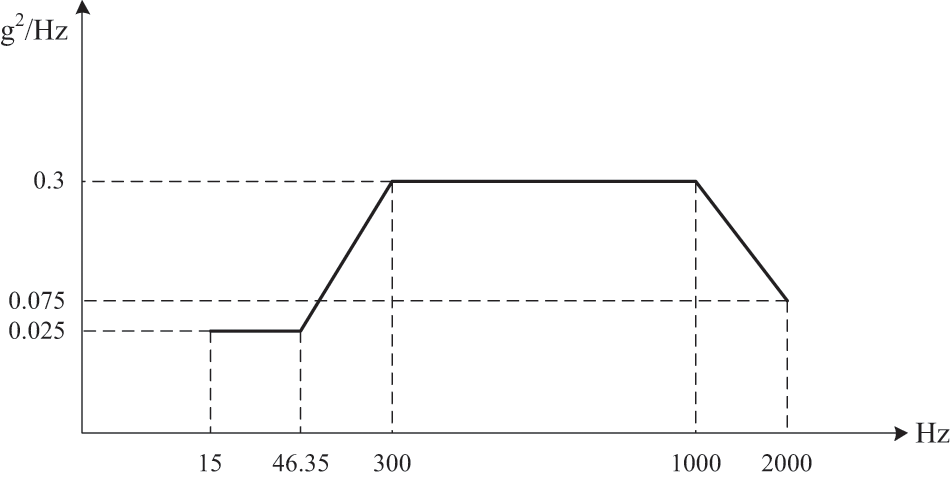
Figure 12: Acceleration power spectral density function of random excitation

In the current state of the AHPS (i.e., when the design variable is at the initial value and the random variable value is at parameter 1), the maximum value of the stress response and displacement response are 2.12 × 107 (Pa) and 3.89 × 10−4 (m), as shown in Figs. 13 and 14, respectively.

Figure 13: Stress response before optimization

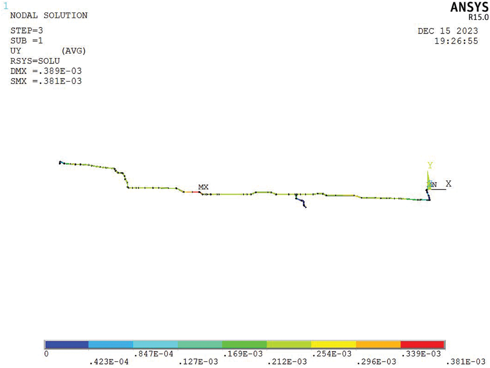
Figure 14: Displacement response before optimization

Both stress and the displacement responses affect the safety of an AHPS. To improve further improve the reliability of the AHPS further, the following RBDO model is established:

Find d∗={d1∗,d2∗,…,d28∗}Smax(d∗)=Min Smax(d∗,xc)subject to R=Pr(Dmax(d,x)−ε≤0)≥Rtadil≤di≤diu  i=1,2,…,28(33)

In Eq. (33), Smax denotes the maximum stress response, d∗ represent the optimal design variable, xc is the mean value of the random variables (i.e., parameter 1 shown in Table 7) and Dmax is the maximum displacement response. It is noteworthy that unlike the previous three examples in which the objective function is only a function of design variables, Smax(d,x) contains both design variables and random variables. Therefore, Eq. (33) cannot be directly solved by the proposed method. Because random variables only affect the reliability constraints, it is reasonable to replace Smax(d,x) with Smax(d∗,xc) as the objective function. Given the threshold ε and target reliability Rta of 4 × 10−4 (m) and 0.999, respectively, based on PRO, the optimization process and results are presented in Fig. 15 and Table 8, respectively.

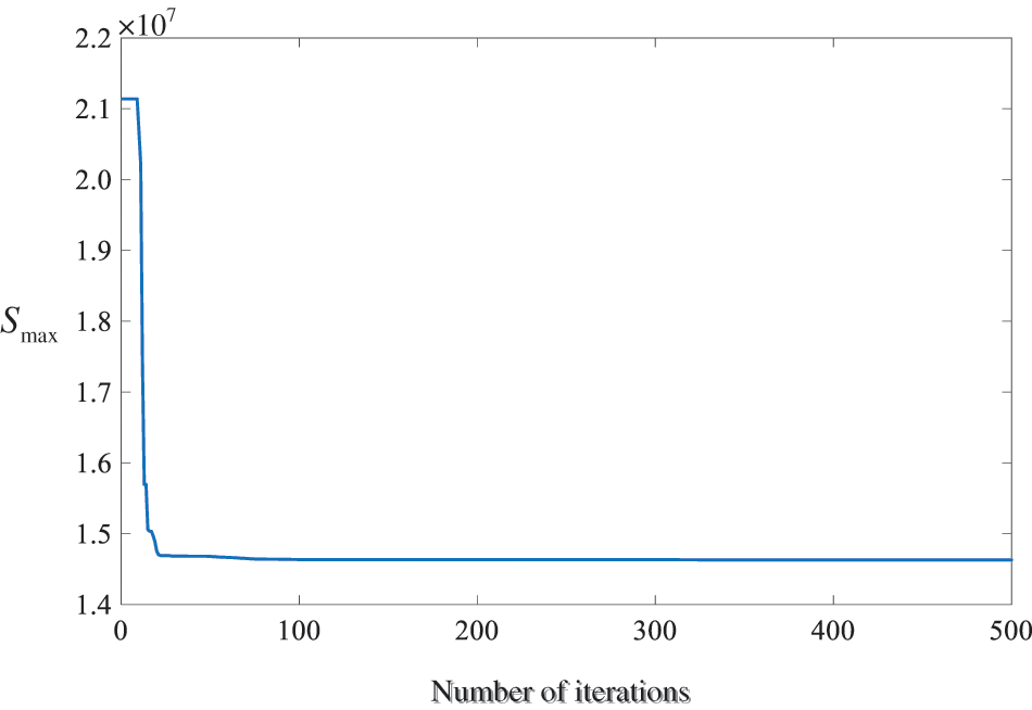
Figure 15: Optimization process of the AHPS

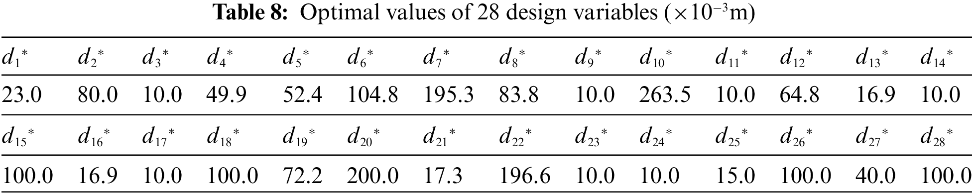
For practical problems, only PM-PRO is used to perform optimization analysis because it has better global stability than SQP. When comparing Figs. 13 and 16, one can see that the result is reduced from 2.12 × 107 (Pa) to 1.48 × 107 (Pa) through the RBDO design, representing a reduction of approximately 31.19%. Simultaneously, as a reliability constraint, the displacement response is reduced from 3.89 × 10−4 (m) to 2.73 × 10−4 (m), representing a reduction of approximately 27.51% which can be found in the comparison between Figs. 14 and 17. When substituting the initial value in Table 6 and the optimal values in Table 8 into Eq. (33), the resulting reliability levels are 0.9980 and 0.9991, respectively, indicating that the optimized reliability level satisfies the requirements. Because there are only one reliability constraint in this reliability optimization problem, the number of function evaluations used to approximate the performance function in the reliability constraint is 3 × 8 + 28 × 5 = 164. It is noteworthy that the sample size used to fit each univariate function is 5. This value is selected based on the empirical results obtained from several previous examples (i.e., when the sample size is greater than 4, engineering accuracy can be guaranteed). It should be noted that the RBDO of this AHPS is different from previous optimization problems, where the objective functions are explicit functions that does not need require additional computation. The optimization objective in the AHPS is an implicit function and additional calculations are required for each iteration. To reduce the computational cost, the implicit optimization target is approximated utilizing Lagrange interpolation and the concrete process is similar to that of the optimization constraint. The number of function calls required to approximate the implicit objective function is 28 × 5 = 140 and the error is approximately 1.22%. Therefore, the total number of function calls is 304 for the RBDO of the AHPS.

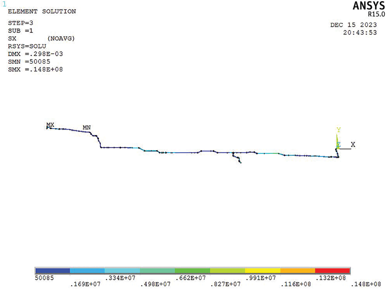
Figure 16: Stress response after optimization

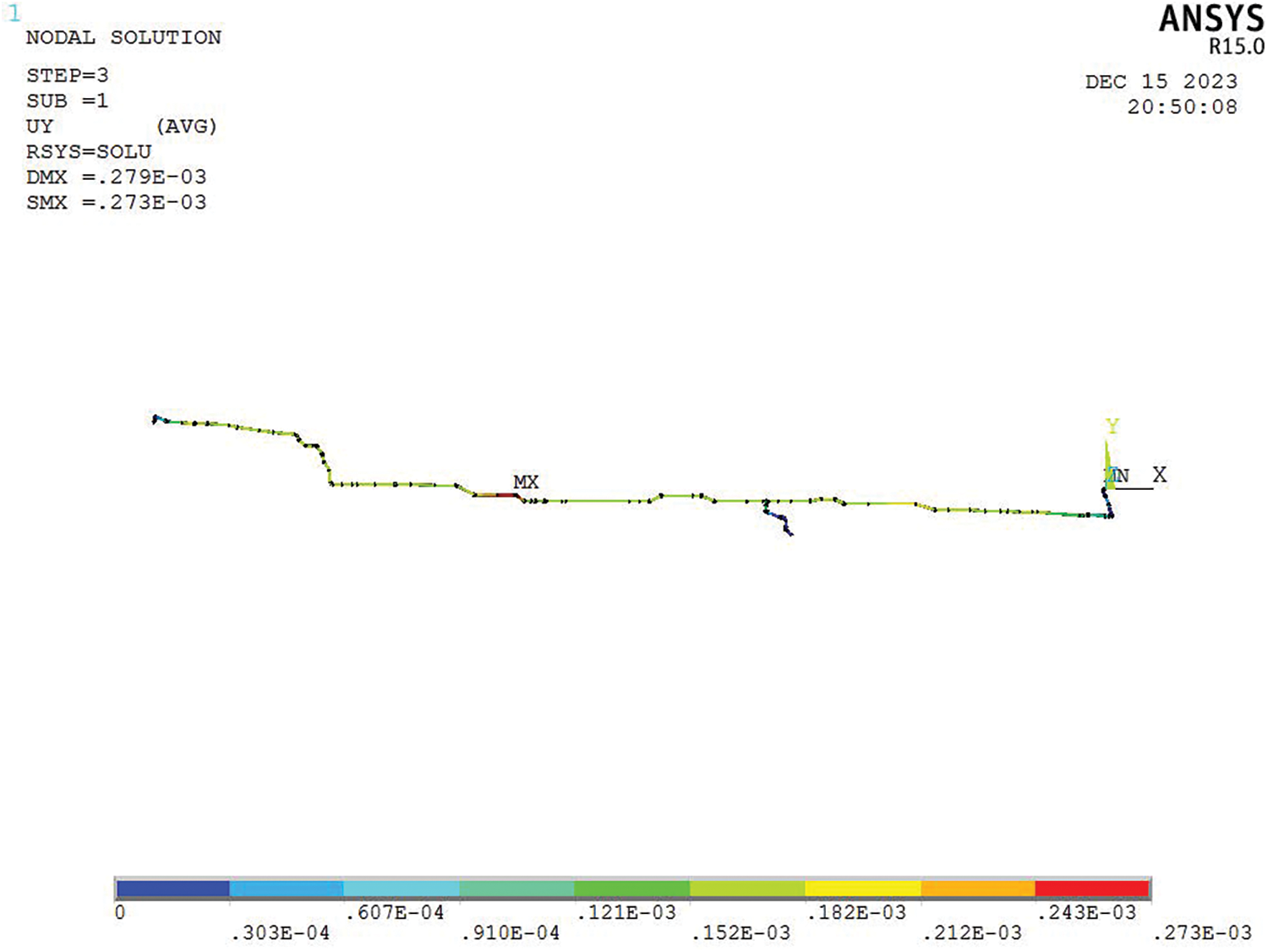
Figure 17: Displacement response after optimization

6  Conclusions

In this study, the RBDO model is completely decoupled into a general constrained optimization problem based on MDRM and WPEM, and Lagrange interpolation is used to approximate a univariate function. Therefore, the RBDO problem is transformed into a general constrained optimization problem. Because the transformed model is a proxy model, no additional computation is required for optimization analysis following transformation. As a result, the computational cost of the proposed method mainly depends on decoupling and the approximation of reliability constraints. In the first example with a single reliability constraint, the number of function calls is 14 and the error is 5.92%. The number of function calls is only 38 for the second example with four reliability constraints. The function calls are 89 and 164 for two finite element examples with 15 and 36 variables, respectively. These examples fully demonstrated the excellent practicability, efficiency, and accuracy of the proposed method.

Acknowledgement: The authors disclosed receipt of the following financial support for the research, authorship and/or publication of this article: This work was supported by the Innovation Fund Project of the Gansu Education Department.

Funding Statement: The authors disclosed receipt of the following financial support for the research, authorship and/or publication of this article: This work was supported by the Innovation Fund Project of the Gansu Education Department (Grant No. 2021B-099).

Author Contributions: Wang Wenxuan and Zhang Feng are mainly responsible for theoretical exploration and subsequent syntax modification; Wang Xiaoyi is responsible for theoretical derivation, algorithm programming and paper writing; Chang Xinyue and Qiao Zijie are responsible for example verification and analysis.

Availability of Data and Materials: Algorithm code and related data are available via email: wxwangd@163.com.

Conflicts of Interest: The authors declare that they have no conflicts of interest to report regarding the present study.

References

1. Zhang, H., Song, L., Bai, G. (2023). Active kriging-based adaptive importance sampling for reliability andsensitivity analyses of stator blade regulator. Computer Modeling in Engineering & Science, 134(3), 1871–1897. https://doi.org/10.32604/cmes.2022.021880 [Google Scholar] [CrossRef]

2. Li, X. Q., Song, L. K., Choy, Y. S., Bai, G. C. (2023). Multivariate ensembles-based hierarchical linkage strategy for system reliability evaluation of aeroengine cooling blades. Aerospace Science and Technology, 138, 108325. [Google Scholar]

3. Li, X. Q., Song, L. K., Bai, G. C. (2022). Deep learning regression-based stratified probabilistic combined cycle fatigue damage evaluation for turbine bladed disks. International Journal of Fatigue, 159, 106812. [Google Scholar]

4. Shamsaddinlou, A., Shirgir, S., Hadidi, A., Azar, B. F. (2023). An efficient reliability-based design of TMD $ MTMD in nonlinear structures under uncertainty. Structures, 51, 258–274. [Google Scholar]

5. Biswas, R., Sharma, D. (2023). Chaos control assisted single-loop multi-objective reliability-based design optimization using differential evolution. Swarm and Evolutionary Computation, 81, 101340. https://doi.org/10.1016/j.swevo.2023.10134 [Google Scholar] [CrossRef]

6. Zhang, C., Shafieezadeh, A. (2021). A quantile-based sequential approach to reliability-based design optimization via error-controlled adaptive Kriging with independent constraint boundary sampling. Structural and Multidisciplinary Optimization, 63(5), 2231–2252. [Google Scholar]

7. Yang, F., Ren, J. (2020). Reliability analysis based on optimization random forest model and MCMC. Computer Modeling in Engineering & Sciences, 125(2), 801–814. https://doi.org/10.32604/cmes.2020.08889 [Google Scholar] [CrossRef]

8. He, J., Luo, Y. (2020). A Bayesian updating method for non-probabilistic reliability assessment of structures with performance test data. Computer Modeling in Engineering & Sciences, 125(2), 777–800. https://doi.org/10.32604/cmes.2020.010688 [Google Scholar] [CrossRef]

9. Wang, N., Zhang, H., Lv, R., Guo, Y., Zhu, P. (2022). An investigation of reliability optimization in standby systems. Proceedings of the Institution of Mechanical Engineers, Part O: Journal of Risk and Reliability, 236(2), 237–247. [Google Scholar]

10. Wang, X., Wang, R., Wang, L., Chen, X., Geng, X. (2018). An efficient single-loop strategy for reliability-based multidisciplinary design optimization under non-probabilistic set theory. Aerospace Science and Technology, 73, 148–163. [Google Scholar]

11. Jiang, C., Qiu, H., Gao, L., Cai, X., Li, P. (2017). An adaptive hybrid single-loop method for reliability-based design optimization using iterative control strategy. Structural and Multidisciplinary Optimization, 56(6), 1271–1286. [Google Scholar]

12. Keshtegar, B., Hao, P. (2018). Enhanced single-loop method for efficient reliability-based design optimization with complex constraints. Structural and Multidisciplinary Optimization, 57(4), 1731–1747. [Google Scholar]

13. Li, X., Meng, Z., Chen, G., Yang, D. (2019). A hybrid self-adjusted single-loop approach for reliability-based design optimization. Structural and Multidisciplinary Optimization, 60(5), 1867–1885. [Google Scholar]

14. Meng, Z., Yang, D., Zhou, H., Wang, B. P. (2018). Convergence control of single loop approach for reliability-based design optimization. Structural and Multidisciplinary Optimization, 57(3), 1079–1091. [Google Scholar]

15. Lim, J., Lee, B. (2016). A semi-single-loop method using approximation of most probable point for reliability-based design optimization. Structural and Multidisciplinary Optimization, 53(4), 745–757. [Google Scholar]

16. Wauters, J., Couckuyt, I., Degroote, J. (2021). ESLA: A new surrogate-assisted single-loop reliability-based design optimization technique. Structural and Multidisciplinary Optimization, 63(6), 2653–2671. [Google Scholar]

17. Singh, J., Cheng, J. C., Anumba, C. J. (2021). BIM-based approach for automatic pipe systems installation coordination and schedule optimization. Journal of Construction Engineering and Management, 147(11), 04021143. [Google Scholar]

18. Li, G., Yang, H., Zhao, G. (2020). A new efficient decoupled reliability-based design optimization method with quantiles. Structural and Multidisciplinary Optimization, 61(2), 635–647. [Google Scholar]

19. Yan, W., Deng, L., Zhang, F., Li, T., Li, S. (2019). Probabilistic machine learning approach to bridge fatigue failure analysis due to vehicular overloading. Engineering Structures, 193, 91–99. [Google Scholar]

20. Ren, S., Chen, G., Li, T., Chen, Q., Li, S. (2018). A deep learning-based computational algorithm for identifying damage load condition: An artificial intelligence inverse problem solution for failure analysis. Computer Modeling in Engineering & Sciences, 117(3), 287–307. https://doi.org/10.31614/cmes.2018.04697 [Google Scholar] [CrossRef]

21. Shi, Y., Lu, Z., Xu, L., Zhou, Y. (2020). Novel decoupling method for time-dependent reliability-based design optimization. Structural and Multidisciplinary Optimization, 61(2), 507–524. [Google Scholar]

22. Zhang, F., Luo, Y. (2021). Introduction to the special issue on novel methods for reliability evaluation and optimization of complex mechanical structures. Computer Modeling in Engineering & Sciences, 126(2), 711–713. https://doi.org/10.32604/cmes.2021.015567 [Google Scholar] [CrossRef]

23. Deng, K., Song, L. K., Bai, G. C., Li, X. Q. (2022). Improved Kriging-based hierarchical collaborative approach for multi-failure dependent reliability assessment. International Journal of Fatigue, 160, 106842. [Google Scholar]

24. Zhang, H., Song, L. K., Bai, G. C., Li, X. Q. (2022). Active extremum Kriging-based multi-level linkage reliability analysis and its application in aeroengine mechanism systems. Aerospace Science and Technology, 131, 107968. [Google Scholar]

25. Chen, Z., Qiu, H., Gao, L., Su, L., Li, P. (2013). An adaptive decoupling approach for reliability-based design optimization. Computers & Structures, 117, 58–66. [Google Scholar]

26. Zou, T., Mahadevan, S. (2006). A direct decoupling approach for efficient reliability-based design optimization. Structural and Multidisciplinary Optimization, 31(3), 190–200. [Google Scholar]

27. Wang, W., Xue, H., Kong, T. (2020). An efficient hybrid reliability analysis method for structures involving random and interval variables. Structural and Multidisciplinary Optimization, 62(1), 159–173. [Google Scholar]

28. Wang, W., Gao, H., Zhou, C. (2019). Extending the global reliability sensitivity analysis to the systems under double-stochastic uncertainty. Advances in Structural Engineering, 22(3), 626–640. [Google Scholar]

29. Huang, X., Li, Y., Zhang, Y., Zhang, X. (2018). A new direct second-order reliability analysis method. Applied Mathematical Modelling, 55, 68–80. [Google Scholar]

30. Yang, Y. (2013). Polynomial curve fitting and lagrange interpolation. Mathematics and Computer Education, 47(3), 224–230. [Google Scholar]

31. Zhang, X., Pandey, M. D. (2013). Structural reliability analysis based on the concepts of entropy, fractional moment and dimensional reduction method. Structural Safety, 43, 28–40. [Google Scholar]

32. Wang, W., Wang, X. (2021). An efficient variance-based global sensitivity index based on C-DRM and Taylor expansion. Proceedings of the Institution of Mechanical Engineers, Part E: Journal of Process Mechanical Engineering, 235(4), 887–898. [Google Scholar]

33. Strömberg, N. (2017). Reliability-based design optimization using SORM and SQP. Structural and Multidisciplinary Optimization, 56(3), 631–645. [Google Scholar]

34. Zhou, C., Lu, Z., Li, W. (2015). Sparse grid integration based solutions for moment-independent importance measures. Probabilistic Engineering Mechanics, 39, 46–55. [Google Scholar]

35. Büskens, C., Maurer, H. (2000). SQP-methods for solving optimal control problems with control and state constraints: Adjoint variables, sensitivity analysis and real-time control. Journal of Computational and Applied Mathematics, 120(1–2), 85–108. [Google Scholar]

36. Liu, B., Wang, L., Jin, Y. H., Tang, F., Huang, D. X. (2005). Improved particle swarm optimization combined with chaos. Chaos Solitons & Fractals, 25(5), 1261–1271. [Google Scholar]

37. Dubourg, V., Sudret, B., Bourinet, J. M. (2011). Reliability-based design optimization using kriging surrogates and subset simulation. Structural and Multidisciplinary Optimization, 44(5), 673–690. [Google Scholar]

38. Li, M., Sadoughi, M., Hu, C., Hu, Z., Eshghi, A. T. et al. (2019). High-dimensional reliability-based design optimization involving highly nonlinear constraints and computationally expensive simulations. Journal of Mechanical Design, 141(5), 051402. [Google Scholar]

39. Wang, W., Zhou, C., Gao, H., Zhang, Z. (2018). Application of non-probabilistic sensitivity analysis in the optimization of aeronautical hydraulic pipelines. Structural & Multidisciplinary Optimization, 57, 2177–2191. [Google Scholar]