
 Submit a Paper
 Propose a Special lssue
 Open Access
ARTICLE

A Novel Method for Linear Systems of Fractional Ordinary Differential Equations with Applications to Time-Fractional PDEs
1 A. Pidhornyi Institute of Mechanical Engineering Problems of NAS of Ukraine, Kharkiv, 61046, Ukraine
2 College of Mechanics and Materials, Hohai University, Nanjing, 211100, China
3 Nanjing Hydraulic Research Institute, Nanjing, 210029, China
4 Shigatse Everest Urban Investment and Development Group Co, Ltd., 857000, China
* Corresponding Authors: Yuhui Zhang. Email: ; Jun Lu. Email:
(This article belongs to the Special Issue: New Trends on Meshless Method and Numerical Analysis)
Computer Modeling in Engineering & Sciences 2024, 139(2), 1583-1612. https://doi.org/10.32604/cmes.2023.044878
Received 10 August 2023; Accepted 17 November 2023; Issue published 29 January 2024
 View Full Text
 Download PDF
Abstract
This paper presents an efficient numerical technique for solving multi-term linear systems of fractional ordinary differential equations (FODEs) which have been widely used in modeling various phenomena in engineering and science. An approximate solution of the system is sought in the form of the finite series over the Müntz polynomials. By using the collocation procedure in the time interval, one gets the linear algebraic system for the coefficient of the expansion which can be easily solved numerically by a standard procedure. This technique also serves as the basis for solving the time-fractional partial differential equations (PDEs). The modified radial basis functions are used for spatial approximation of the solution. The collocation in the solution domain transforms the equation into a system of fractional ordinary differential equations similar to the one mentioned above. Several examples have verified the performance of the proposed novel technique with high accuracy and efficiency.Keywords
A novel numerical method for solving a linear system of fractional ordinary differential equations (FODEs).
is proposed in this paper. Here:
where
where
The equations similar to (1) often arise in the modeling of various physical phenomena such as the models of pollution in systems of lakes [3–5], of processing the Magnetic Resonance Imaging (MRI) data [6], of the spread of infections [7,8], and also in modeling the nuclear magnetic resonance [9,10]. Recently such problems have become very relevant due to the widespread use of the fractional-order mathematical model of the COVID-19 disease [11–14].
Besides, as is shown below, based on this technique an effective method for solving multi-term time fractional partial differential equations (TFPDEs) of the type
can be developed. Here
is a spatial differential operator of the second order defined for
– the time-fractional sub-diffusion equation [15]
– the time-fractional telegraph equation [16–18]
– the multi-term time-fractional diffusion and diffusion-wave equations [19–21]
– the time-fractional modified anomalous sub-diffusion equation [22–26]
It has been shown by many researchers that the fractional equations are more suitable for modeling some real-world applications compared with the equations of the integral order. The reviews of some real-world applications of the fractional equations were provided by Almeida et al. [27] and Sun et al. [28], in physics [29], solid mechanics [30], and fluid mechanics [31]. The application of fractional equations can also be noted in the recently published books [32,33] and we refer readers to them and to the references therein.
The exact solutions of the fractional equations are critically important for revealing complex physical phenomena. Some well-known analytical methods have been proposed for this goal: the Laplace transform method [34,35], the Green function method [36], the Fourier transform method [37], the variational iteration method [38], the Adomian decomposition method [39], the method of separating variables [40], etc.
However, because analytical solutions are available only for a narrow class of fractional problems, a great number of numerical techniques have been developed. Currently, the finite difference (FD) and finite element (FE) techniques are still the most useful tools in this field.
A survey of the FD methods for solving FODEs and fractional PDEs was presented by Li et al. in [41]. Some non-standard FD techniques were proposed to solve complex fractional systems in [42–44]. The fast FD methods for the fractional equations were proposed for solving 2D/3D space-fractional diffusion equations in [45,46]. Similar fast FD techniques were proposed for distributed-order space-fractional problems in [47], for parameters identifying problems governed by fractional equations in [48], for time-dependent space-fractional diffusion equations with fractional boundary conditions in [49], for the nonlinear fractional wave equation in [50], for fractional equations with singularity in [51], etc. The FE techniques also are the most commonly used for solving fractional equations. The FE approach was used to solve 1D fractional equations in [52,53] and for 2D fractional equations in [54–56]. Many works focus on the error analysis of the FE methods such as [57–59].
Recently meshless methods have become the focused issues of the researchers in science and engineering. The meshless methods can be divided into two groups: the pure collocation techniques [60–63] and the methods based on the integration [64–67]. To improve the accuracy of the meshless methods combinations with semi-analytical techniques have been proposed. The Laplace transform method has been coupled with the Adomian decomposition method in [68]. The analytical and semi-analytical solutions of the time-fractional Cahn–Allen equation have been studied by Khater et al. in [69]. A semi-analytical solution for the time-fractional diffusion equation has been developed by Kazem et al. in [70]. The homotopy analysis transform method [71] and the fundamental solution method [72] belong to the same group of techniques. Five semi-analytical techniques for solving the fractional nonlinear telegraph equation have been studied in [73].
In this paper, a new semi-analytical meshless technique-the backward substitution method (BSM) [74,75] is proposed to solve multi-term linear systems of FODEs. Based on the method provided a flexible and efficient numerical technique is constructed to solve the TFPDE (4). Applying the collocation approach, the original TFPDE is transformed into the system of FODEs which can be handled by the proposed new technique. The performance of this approach has been thoroughly examined by typical numerical examples. The test results are compared with the exact solutions and with the data obtained by other numerical techniques.
The rest of the paper is organized as follows. The detailed scheme of the BSM for solving the system of FODEs is formulated in Section 2. The scheme for solving the TFPDEs is presented in Section 3. The numerical examples are given in Section 4. Finally, some conclusions are briefly discussed in Section 5.
2 Backward Substitution Method for FODEs
In this section, we propose a novel numerical scheme for solving the system (1) subjected to the initial conditions (ICs):
Let us define a new vector-function
where
is a known vector function of time. Substituting the relation (11) into the governing Eq. (1), one gets the equation for the new variable
where
In should be noted that
Let us rewrite the system in the form:
Let
where
Throughout the paper, we use the generalized power functions or the Müntz polynomials basis (MPB) [76,77]. A fractional derivative of a Müntz polynomial is again a Müntz polynomial. This is a crucial feature of this base for using it in the collocation methods for Fractional Differential Equations (FDEs). So, we take
as the basis functions and the solution is sought in the class of functions which can be approximated by the MPB and for which there exist fractional derivatives of the original Eq. (1).
Here
Under the condition (17) the system (16) can be written in the form:
Suppose that the matrix
As it follows from Eq. (3) the analytical expression
satisfies the FODE
Because
Therefore, the linear combination
is the semi-analytical solution of Eq. (20) for any
or
If the Eq. (26) is fulfilled at any time moment
In practical calculations, we consider the truncated series
as an approximate solution of the problem (13), (15). It satisfies the truncated analog of the system (20):
and the unknown vectors
where
The collocation system (29) can be written in the compact form:
where
The collocation matrix
Here M is the number of the Müntz polynomials
The matrices
are also the
So, the algorithm of the solution of the system (31) is as follows:
Step 1. Choose the parameter of the Müntz polynomials basis,
Step 2. Choose the number of the Müntz polynomials M in the approximate solution.
Step 3. Define the functions
Step 4. Calculate the collocation matrix
Step 5. Calculate the vector of the right hand side
Step 6. Solve the collocation system (31) for
Step 7. Getting the functions
Step 8. Obtain the approximate solution of the original problem (1), (10) as the sum
Let us consider the TFPDE of the form:
subjected to the Dirichlet boundary conditions (BCs)
where
Let us define the new function
where
This function satisfies the equation
under the BCs
and zero ICs
Here
Note: The last terms in (44) can be expressed in the analytical form. Indeed,
where the derivative
So, (44) is the analytical expression.
Let us define the function
which satisfies the BCs (41), (42) and introduce the new variable
The function
where
It is easily to prove that the function
Let us choose a set of linearly independent functions
where
Based on the numerical experiments carried out we fix the shape parameter
We define the modified basis functions
where the coefficients
As a result we get the linear system
for each pair of the coefficients
We seek the solution of the Eq. (49), in the form of the linear series over the modified basis functions
Substituting Eq. (59) into Eq. (49) we get
Let
We take the centers of the RBFs as the collocation points:
where
and
So, the system (62) takes the same form as the linear system of FODEs (1) and can be solved by the algorithm described in Section 2. It should be noted that taking into account (51), the vector
It means that
where
Let us consider TFPDE (4) with a nonlinear term
Let
transforms (68) into a sequence of linear TFPDEs each of those can be solved by the technique described above. As a result, we get the iteration procedure. The iterations are stopped with the control of the error
In this section several numerical examples are provided to show the accuracy of the proposed scheme. To demonstrate the performance of this technique we consider the different types of errors for systems of FODEs and TFPDEs.
The errors (69), (70) are used in solving systems of the FODEs to estimate the approximate solution of each component of the vector
The errors (71), (72) are used in solving TFPDE (36) with the BCs (37) and the ICs (38). The error
4.1 Numerical Experiments for Systems of FODEs
Example 4.1 Let us consider the system given in [35]
with the general exact solution
where
and
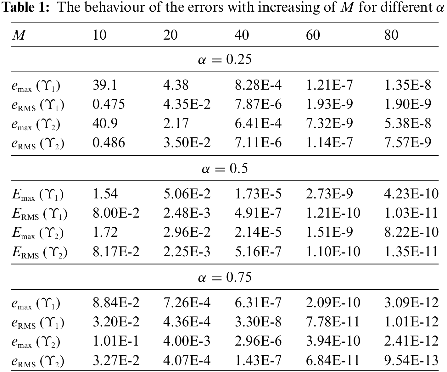
Example 4.2 Let us consider the system described in [35]
with the general exact solution
where
and
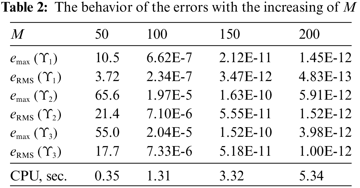
Example 4.3 Consider the following initial value problem for the inhomogeneous Bagley–Torvik equation [81]
with the exact solution
with the initial condition
where the solution of the original Bagley–Torvik equation
According to the method described above, the approximate solution can be written in the form:
where
Thus, the approximate solution (83) contains the exact solution
The data placed in Table 3 demonstrate that if the approximate solution (83) contains the exact solution
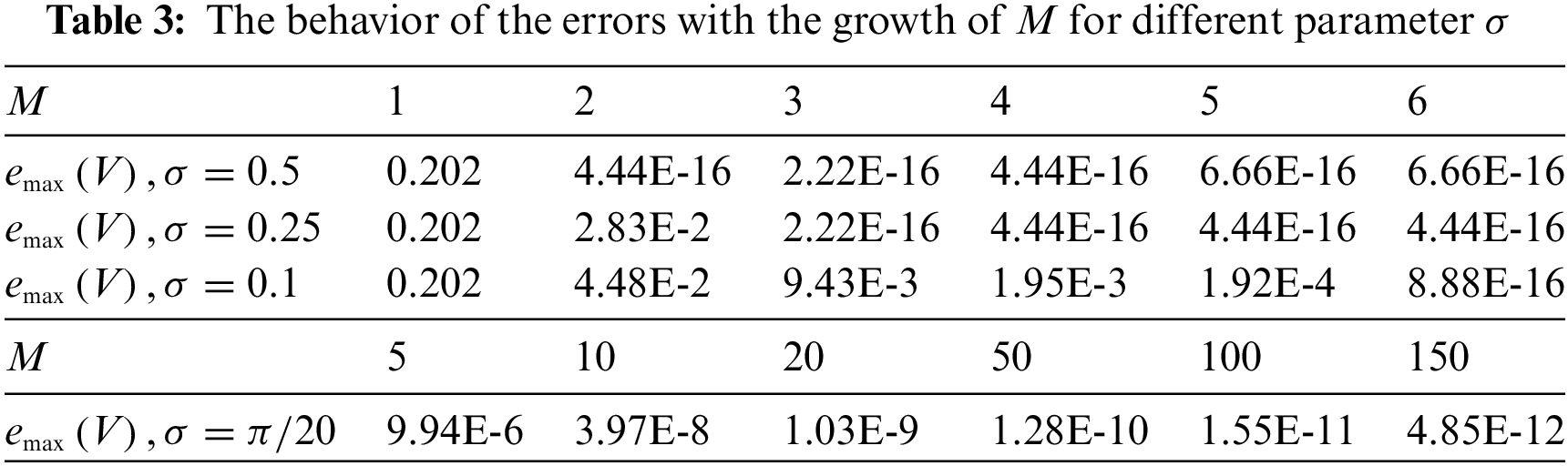
The data placed in the last rows of Table 3 correspond to the general case when the information of the solution is absent. We take
The same problem has been studied in [81] on the time interval
Table 4 shows the results of the calculation by the proposed method on the time interval

Example 4.4 Let us consider the multi-term system with time-dependent matrices
The ICs are
Her
The vector
The data placed in Table 5 demonstrate the behavior of the error of the approximate solution with the growth of M for

Similar to (83), (84), the approximate solution can be written in the form:
where
In this case we use the additional information that the components of the solution
Table 6 demonstrates a dramatic decrease in the errors with the growth of M for this special choice of

4.2 Numerical Experiments for TFPDEs
Example 4.5 Let us consider the multi-term TFPDE [83]
Here the source term
Fig. 1 and Table 7 show the behavior of the errors of the approximate solution as the functions of N (see (59)) with the fixed M. For
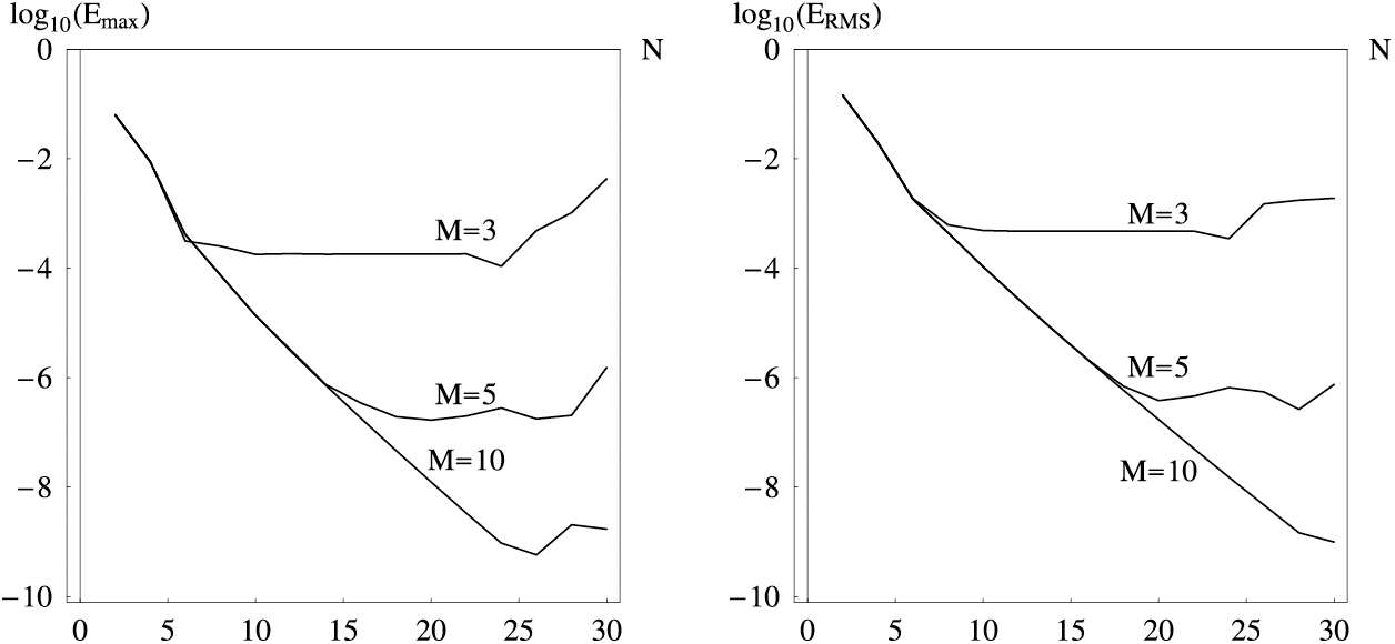
Figure 1: The maximal absolute

Fig. 2 and Table 8 show the behavior of the errors as functions of M with the fixed N. It is evident that the proposed scheme converges fast with the increase of M. For the larger M more accurate results can be obtained. The same problem was studied by Jin et al. in [83] using the Galerkin FE method and FD discretization of the time-fractional derivatives. Using
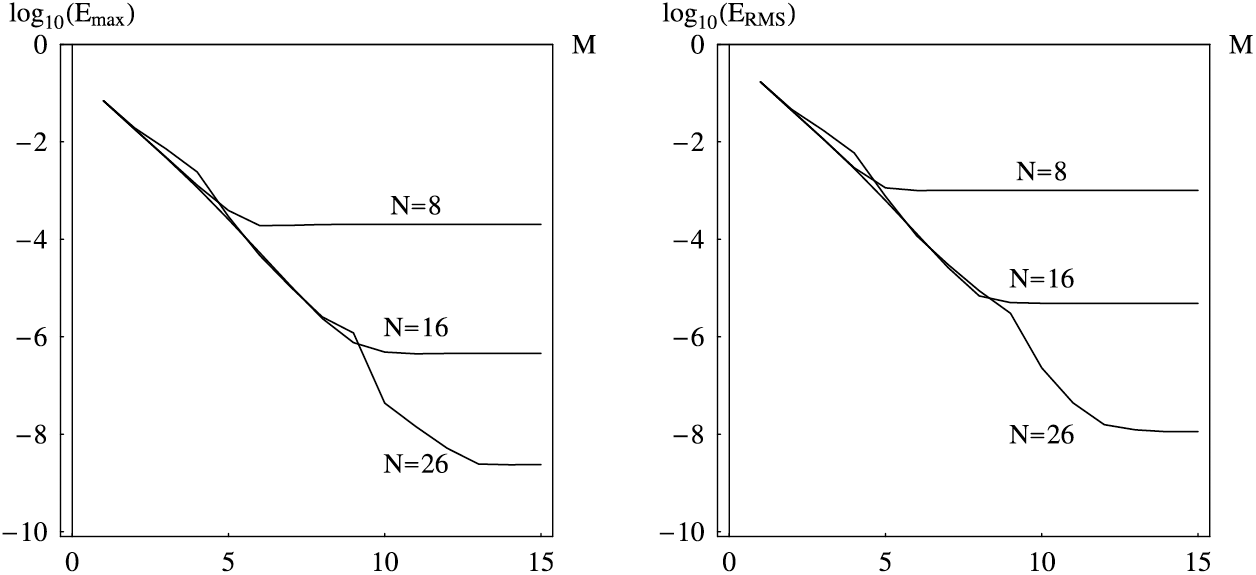
Figure 2: The maximal absolute

Example 4.6 Let us consider the multi-term TFPDE
with the spatial operator
Table 9 shows the errors, convergence order, and CPU time as the functions of N with the fixed M. The data also are illustrated by the graphics in Fig. 3. With increasing of N the proposed method converges fast, and we can obtain the errors around

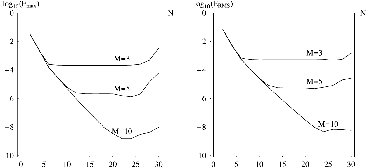
Figure 3: The maximal absolute
Table 10 and Fig. 4 show the errors vs. M with the fixed N to verify the performance of the proposed scheme. The order of convergence is larger than 3.

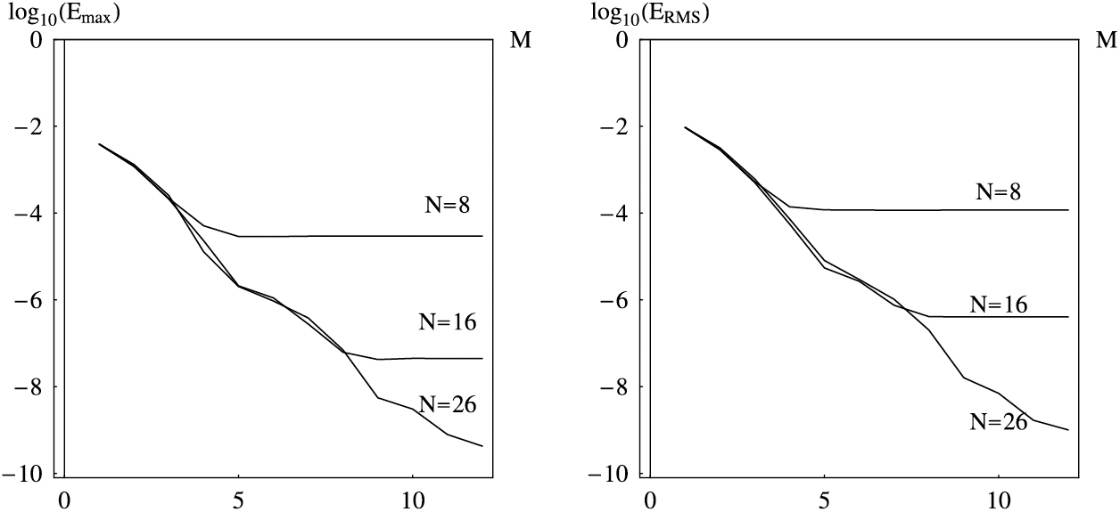
Figure 4: The maximal absolute
Example 4.7 In the following examples we consider three cases for
Case 1: Consider the following equation:
Here we have
The boundary conditions are
The exact solution of the problem is
Case 2: Consider the following equation:
with the spatial operator
The boundary conditions are
The exact solution of the problem is
Case 3: Consider the following equation:
with the spatial operator
The boundary conditions are
The exact solution of the problem is
Tables 11, 12 show the errors with increasing of N with the fixed M. It is evident that the proposed scheme provides very accurate results. Furthermore, for a small number of N, we can also get moderately accurate results with errors around

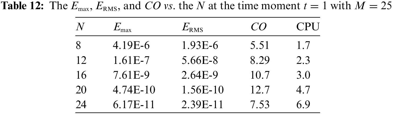

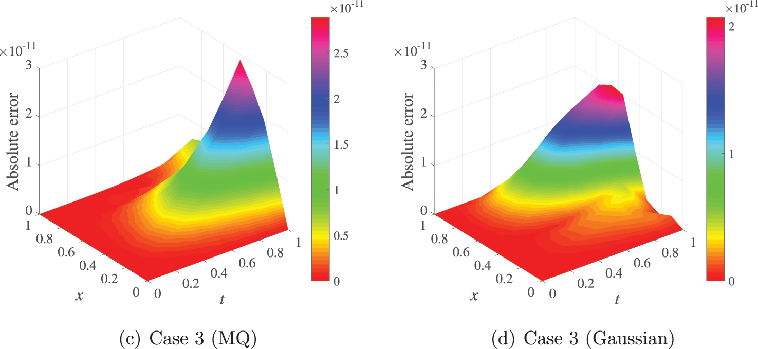
Figure 5: The domain absolute errors

Example 4.8 Consider the nonlinear time-fractional the Huxley-Burgers’ equation of the following form:
The Dirichlet BCs and IC conform to the exact solution
Tables 14, 15 and Fig. 6 show the behaviour of the errors with the growth of N and the fixed M. The data are obtained after 3 iterations of the quazilinearization procedure. The same problem was considered by Hadhoud et al. in [84] using a numerical technique based on the cubic B-spline collocation method and the mean value theorem for integrals. The maximal absolute errors obtained there for the mesh size


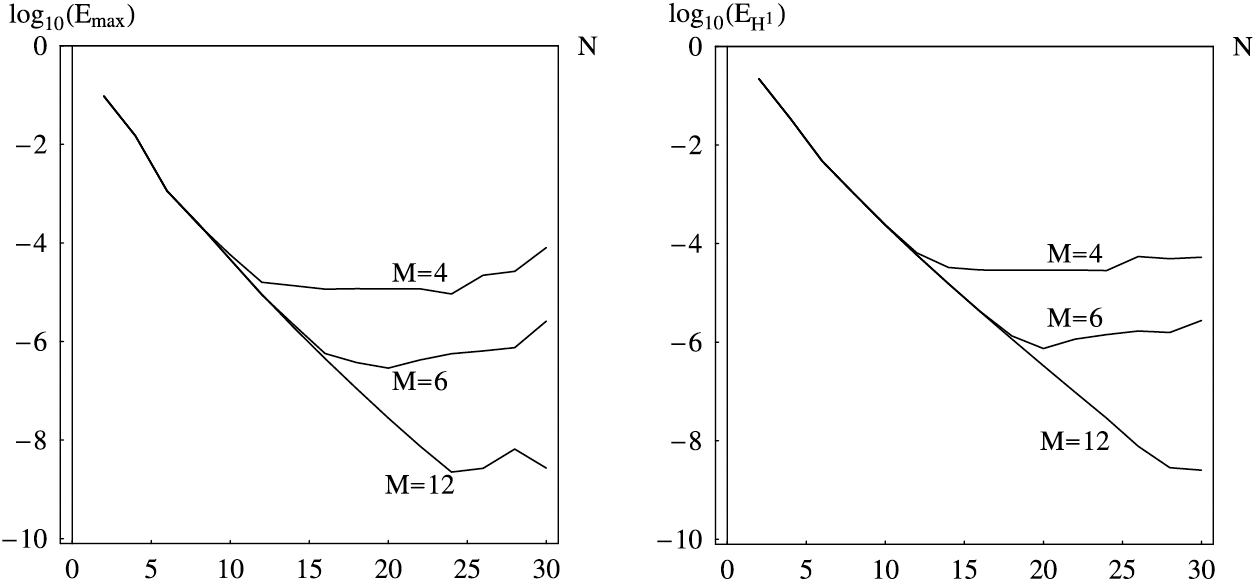
Figure 6: The maximal absolute
Example 4.9 Consider the TFPDE
The source function
Table 16 shows the behavior of the errors with the growth of N with the fixed
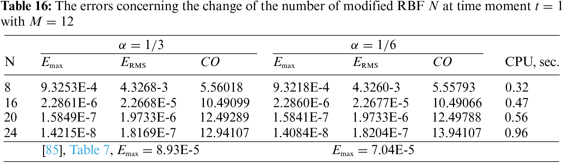
This paper presents a new meshless technique for solving multi-term linear systems of fractional equations. These systems have been used in modeling various phenomena in different branches of engineering and science. Using substitution (11), we transform the original system into the one for the vector variable
In the authors’ opinion, the main results achieved in the paper are: (1) The effective method for solving systems of the FODEs with time-dependent coefficients has been developed and tested. (2) On the base of this technique the method of solving TFPDEs of the high fractional order has been proposed. The method has been tested on the problems with the highest derivative of the orders:
Some remarks: (1) In this paper the MQ-RBF is mainly used for spatial approximation. However, the last example demonstrates that the Gaussian RBF is suitable for this purpose. The other global RBFs, compactly supported RBFs and B-splines also can be used for spatial approximation in the framework of the proposed technique. (2) Only the Dirichlet BCs are considered in this study. However, the proposed technique can be extended to the problems with the boundary conditions of the general type by some modification of the Eqs. (56)–(58). (3) Only (1 + 1) dimensional problems have been considered. However, using multidimensional RBSs, this approach can be extended to the (2 + 1) and (3 + 1) dimensional problems.
It should be remarked that the limitation of the presented technique is caused by the fast growth of the size of the collocation matrix
To overcome this problem we presuppose the use of a localized scheme of the spatial approximation based on the compactly supported radial basis functions (CSRBF) in the future to avoid dense and ill-conditioning matrices.
To overcome the problems of calculations on the large time interval
Let
Solving the Eq. (1) in the first subinterval
which can be used as the initial data for solving the equation in the second subinterval
We get the equation for the unknown vector
with the ICs
Then, the vectors
Acknowledgement: The authors wish to express their appreciation to the reviewers for their helpful suggestions whose efforts have helped to improve the quality of this paper.
Funding Statement: This research was funded by the National Key Research and Development Program of China (No. 2021YFB2600704), the National Natural Science Foundation of China (No. 52171272), and the Significant Science and Technology Project of the Ministry of Water Resources of China (No. SKS-2022112).
Availability of Data and Materials: Sergiy Reutskiy: Methodology and Writing–Original Draft; Yuhui Zhang: Writing–Review & Editing; Jun Lu: Writing–Review & Editing; Ciren Pubu: Validation.
Conflicts of Interest: The authors declare that they have no conflicts of interest to report regarding the present study.
References
1. Podlubny, I. (1999). Fractional differential equations. New York: Academic Press. [Google Scholar]
2. Diethelm, K. (2010). The analysis of fractional differential equations. In: Lecture notes in mathematics, vol. 2004. Berlin: Springer. [Google Scholar]
3. Biazar, J., Farrokhi, L., Islam, M. R. (2006). Modeling the pollution of a system of lakes. Applied Mathematics and Computation, 178(2), 423–430. [Google Scholar]
4. Khader, M. M., El Danaf, T. S., Hendy, A. S. (2013). A computational matrix method for solving systems of high order fractional differential equations. Applied Mathematical Modelling, 37(6), 4035–4050. [Google Scholar]
5. El-Dessoky Ahmed, M. M., Khan, M. A. (2020). Modeling and analysis of the polluted lakes system with various fractional approaches. Chaos, Solitons & Fractals, 134, 109720. [Google Scholar]
6. Qin, S., Liu, F., Turner, I., Vegh, V., Yu, Q. et al. (2017). Multi-term time-fractional Bloch equations and application in magnetic resonance imaging. Journal of Computational and Applied Mathematics, 319, 308–319. [Google Scholar]
7. Cardoso, L. C., Dos Santos, F. L. P., Camargo, R. F. (2018). Analysis of fractional-order models for hepatitis B. Computational and Applied Mathematics, 37, 4570–4586. [Google Scholar]
8. Ding, Y., Ye, H. (2009). A fractional-order differential equation model of HIV infection of CD4+ T-cells. Mathematical and Computer Modelling, 50(3–4), 386–392. [Google Scholar]
9. Magin, R., Feng, X., Baleanu, D. (2009). Solving the fractional order Bloch equation. Concepts in Magnetic Resonance Part A: An Educational Journal, 34(1), 16–23. [Google Scholar]
10. Yu, Q., Liu, F., Turner, I., Burrage, K. (2014). Numerical simulation of the fractional Bloch equations. Journal of Computational and Applied Mathematics, 255, 635–651. [Google Scholar]
11. Xu, C., Yu, Y., Ren, G., Sun, Y., Si, X. (2023). Stability analysis and optimal control of a fractional-order generalized SEIR model for the COVID-19 pandemic. Applied Mathematics and Computation, 457, 128210. https://doi.org/10.1016/j.amc.2023.128210 [Google Scholar] [CrossRef]
12. Batiha, I. M., Momani, S., Ouannas, A. (2022). Fractional-order COVID-19 pandemic outbreak: Modeling and stability analysis. International Journal of Biomathematics, 15(1), 2150090. [Google Scholar]
13. Ndaïrou, F., Area, I., Nieto, J. J., Silva, C. J., Torres, D. F. M. (2021). Fractional model of COVID-19 applied to Galicia, Spain and Portugal. Chaos, Solitons & Fractals, 144, 110652. https://doi.org/10.1016/j.chaos.2021.110652 [Google Scholar] [PubMed] [CrossRef]
14. Ogunrinde, R. B., Nwajeri, U. K., Fadugba, S. E., Ogunrinde, R. R., Oshinubi, K. I. (2021). Dynamic model of COVID-19 and citizens reaction using fractional derivative. Alexandria Engineering Journal, 60, 2001–2012. https://doi.org/10.1016/j.aej.2020.09.016 [Google Scholar] [CrossRef]
15. Zeng, F. H., Li, C. P., Liu, F. W., Turner, I. (2015). Numerical algorithms for time-fractional subdiffusion equation with second-order accuracy. SIAM Journal on Scientific Computing, 37, A55–A78. [Google Scholar]
16. Das, S., Vishal, K., Gupta, P. K., Yildirim, A. (2011). An approximate analytical solution of time-fractional telegraph equation. Applied Mathematics and Computation, 217, 7405–7411. [Google Scholar]
17. Hosseini, V. R., Chen, W., Avazzadeh, Z. (2014). Numerical solution of fractional telegraph equation by using radial basis functions. Engineering Analysis with Boundary Elements, 38, 31–39. [Google Scholar]
18. Mollahasani, N., Mohseni Moghadam, M., Afrooz, K. (2016). A new treatment based on hybrid functions to the solution of telegraph equations of fractional order. Applied Mathematical Modelling, 5–6, 2804–2814. [Google Scholar]
19. Liu, F., Meerschaert, M. M., McGough, R. J., Zhuang, P., Liu, Q. (2013). Numerical methods for solving the multi-term time-fractional wave-diffusion equations. Fractional Calculus and Applied Analysis, 16, 9–25. [Google Scholar] [PubMed]
20. Zheng, M., Liu, F., Anh, V., Turner, I. (2016). A high-order spectral method for the multi-term time-fractional diffusion equations. Applied Mathematical Modelling, 40, 4970–4985. [Google Scholar]
21. Dehghan, M., Safarpoor, M., Abbaszadeh, M. (2015). Two high-order numerical algorithms for solving the multi-term time fractional diffusion-wave equations. Journal of Computational and Applied Mathematics, 290, 174–195. [Google Scholar]
22. Liu, L., Yang, C., Burrage, K. (2009). Numerical method and analytical technique of the modified anomalous subdiffusion equation with a nonlinear source term. Journal of Computational and Applied Mathematics, 231, 160–176. [Google Scholar]
23. Liu, Q., Liu, F., Turner, I., Anh, V. (2011). Finite element approximation for a modified anomalous subdiffusion equation. Applied Mathematical Modelling, 35, 4103–4116. [Google Scholar]
24. Chen, W., Sun, H., Zhang, X., Korošakb, D. (2010). Anomalous diffusion modeling by fractal and fractional derivatives. Journal of Computational and Applied Mathematics, 59, 1754–1758. [Google Scholar]
25. Mohebbi, M., Abbaszadeh, M., Dehghan, M. (2013). A high-order and unconditionally stable scheme for the modified anomalous fractional sub-diffusion equation with a nonlinear source term. Journal of Computational Physics, 240, 36–48. [Google Scholar]
26. Dehghan, M., Abbaszadeh, M., Mohebbi, A. (2016). Legendre spectral element method for solving time fractional modified anomalous sub-diffusion equation. Applied Mathematical Modelling, 40(5–6), 3635–3654. [Google Scholar]
27. Almeida, R., Bastos, N. R. O., Monteiro, M. T. T. (2016). Modeling some real phenomena by fractional differential equations. Mathematical Methods in the Applied Sciences, 239(16), 4846–4855. [Google Scholar]
28. Sun, H., Zhang, Y., Baleanu, D., Chen, W., Chen, Y. (2018). A new collection of real world applications of fractional calculus in science and engineering. Communications in Nonlinear Science and Numerical Simulation, 64, 213–231. [Google Scholar]
29. Hilfer, R. (2000). Applications of fractional calculus in physics. Singapore: World Scientific. [Google Scholar]
30. Rossikhin, Y. A., Shitikova, M. V. (2010). Application of fractional calculus for dynamic problems of solid mechanics: Novel trends and recent results. Applied Mechanics Reviews, 63(1), 010801. [Google Scholar]
31. Kulish, V. V., Lage, J. L. (2002). Application of fractional calculus to fluid mechanics. Journal of Fluids Engineering, 124(3), 803–806. [Google Scholar]
32. Yang, X. J. (2019). General fractional derivatives: Theory, methods and applications. Boca Raton, FL: CRC Press. [Google Scholar]
33. Mainardi, F. (2022). Fractional calculus and waves in linear viscoelasticity: An introduction to mathematical models. Singapore: World Scientific. [Google Scholar]
34. Kexue, L., Jigen, P. (2011). Laplace transform and fractional differential equations. Applied Mathematics Letters, 24(12), 2019–2023. [Google Scholar]
35. Odibat, Z. M. (2010). Analytic study on linear systems of fractional differential equations. Computers & Mathematics with Applications, 59(3), 1171–1183. [Google Scholar]
36. Mamchuev, M. O. (2017). Solutions of the main boundary value problems for the time-fractional telegraph equation by the Green function method. Fractional Calculus and Applied Analysis, 20, 190–211. [Google Scholar]
37. Bailey, D. H., Swarztrauber, P. N. (1991). The fractional Fourier transform and applications. SIAM Review, 33(3), 389–404. [Google Scholar]
38. Das, S. (2009). Analytical solution of a fractional diffusion equation by variational iteration method. Computers & Mathematics with Applications, 57(3), 483–487. [Google Scholar]
39. Momani, S., Odibat, Z. (2006). Analytical solution of a time-fractional Navier-Stokes equation by Adomian decomposition method. Applied Mathematics and Computation, 177(2), 488–494. [Google Scholar]
40. Wu, C., Rui, W. (2018). Method of separation variables combined with homogenous balanced principle for searching exact solutions of nonlinear time-fractional biological population model. Communications in Nonlinear Science and Numerical Simulation, 63, 88–100. [Google Scholar]
41. Li, C., Zeng, F. (2012). Finite difference methods for fractional differential equations. International Journal of Bifurcation and Chaos, 22(4), 1230014. [Google Scholar]
42. Moaddy, K., Momani, S., Hashim, I. (2011). The non-standard finite difference scheme for linear fractional PDEs in fluid mechanics. Computers & Mathematics with Applications, 61(4), 1209–1216. [Google Scholar]
43. Baleanu, D., Zibaei, S., Namjoo, M., Jajarmi, A. (2011). A nonstandard finite difference scheme for the modeling and nonidentical synchronization of a novel fractional chaotic system. Advances in Difference Equations, 2021(1), 308. [Google Scholar]
44. Hajipour, M., Jajarmi, A., Baleanu, D. (2018). An efficient nonstandard finite difference scheme for a class of fractional chaotic systems. Journal of Computational and Nonlinear Dynamics, 13, 021013. [Google Scholar]
45. Wang, H., Basu, T. S. (2012). A fast finite difference method for two-dimensional space-fractional diffusion equations. SIAM Journal on Scientific Computing, 34(5), A2444–A2458. [Google Scholar]
46. Wang, H., Du, N. (2013). A fast finite difference method for three-dimensional time-dependent space-fractional diffusion equations and its efficient implementation. Journal of Computational Physics, 253, 50–63. [Google Scholar]
47. Jia, J., Wang, H. (2018). A fast finite difference method for distributed-order space-fractional partial differential equations on convex domains. Computers & Mathematics with Applications, 75(6), 2031–2043. [Google Scholar]
48. Chen, S., Liu, F., Jiang, X., Turner, I., Burrage, K. (2016). Fast finite difference approximation for identifying parameters in a two-dimensional space-fractional nonlocal model with variable diffusivity coefficients. SIAM Journal on Numerical Analysis, 54(2), 606–624. [Google Scholar]
49. Zhao, M., Wang, H., Cheng, A. (2018). A fast finite difference method for three-dimensional time-dependent space-fractional diffusion equations with fractional derivative boundary conditions. Journal of Scientific Computing, 74, 1009–1033. [Google Scholar]
50. Lyu, P., Liang, Y., Wang, Z. (2020). A fast linearized finite difference method for the nonlinear multi-term time-fractional wave equation. Applied Numerical Mathematics, 151, 448–471. [Google Scholar]
51. Shen, J., Sun, Z., Du, R. (2018). Fast finite difference schemes for time-fractional diffusion equations with a weak singularity at initial time. East Asian Journal of Applied Mathematics, 8(4), 834–858. [Google Scholar]
52. Zhuang, P., Liu, F., Turner, I., Gu, Y. (2014). Finite volume and finite element methods for solving a one-dimensional space-fractional Boussinesq equation. Applied Mathematical Modelling, 38(15–16), 3860–3870. [Google Scholar]
53. Cao, W., Hao, Z., Zhang, Z. (2022). Optimal strong convergence of finite element methods for one-dimensional stochastic elliptic equations with fractional noise. Journal of Scientific Computing, 91(1), 1. [Google Scholar]
54. Zhao, Y., Bu, W., Huang, J., Liu, D. Y., Tang, Y. (2015). Finite element method for two-dimensional space-fractional advection-dispersion equations. Applied Mathematics and Computation, 257, 553–565. [Google Scholar]
55. Bu, W., Tang, Y., Wu, Y. Yang. J. (2015). Finite difference/finite element method for two-dimensional space and time fractional Bloch-Torrey equations. Journal of Computational Physics, 293, 264–279. [Google Scholar]
56. Feng, L., Liu, F., Turner, I., Yang, Q., Zhuang, P. (2018). Unstructured mesh finite difference/finite element method for the 2D time-space Riesz fractional diffusion equation on irregular convex domains. Applied Mathematical Modelling, 59, 441–463. [Google Scholar]
57. Jin, B., Lazarov, R., Pasciak, J., Zhou, Z. (2014). Error analysis of a finite element method for the space-fractional parabolic equation. SIAM Journal on Numerical Analysis, 52(5), 2272–2294. [Google Scholar]
58. Huang, C., Stynes, M. (2021). α-robust error analysis of a mixed finite element method for a time-fractional biharmonic equation. Numerical Algorithms, 87, 1749–1766. [Google Scholar]
59. Li, X., Yang, X., Zhang, Y. (2017). Error estimates of mixed finite element methods for time-fractional Navier-Stokes equations. Journal of Scientific Computing, 70, 500–515. [Google Scholar]
60. Mohebbi, A., Abbaszadeh, M., Dehghan, M. (2013). The use of a meshless technique based on collocation and radial basis functions for solving the time fractional nonlinear Schrodinger equation arising in quantum mechanics. Engineering Analysis with Boundary Elements, 37(2), 475–485. [Google Scholar]
61. Kumar, A., Bhardwaj, A., Kumar, B. V. R. (2019). A meshless local collocation method for time fractional diffusion wave equation. Computers & Mathematics with Applications, 78(6), 1851–1861. [Google Scholar]
62. Faghih, A., Mokhtary, P. (2021). A new fractional collocation method for a system of multi-order fractional differential equations with variable coefficients. Journal of Computational and Applied Mathematics, 383, 113139. https://doi.org/10.1016/j.cam.2020.113139 [Google Scholar] [CrossRef]
63. Hu, W., Fu, Z., Tang, Z., Gu, Y. (2022). A meshless collocation method for solving the inverse Cauchy problem associated with the variable-order fractional heat conduction model under functionally graded materials. Engineering Analysis with Boundary Elements, 140, 132–144. [Google Scholar]
64. Habibirad, A., Hesameddini, E., Azin, H., Heydari, M. H. (2023). The direct meshless local Petrov-Galerkin technique with its error estimate for distributed-order time fractional Cable equation. Engineering Analysis with Boundary Elements, 150, 342–352. [Google Scholar]
65. Abbaszadeh, M., Dehghan, M. (2020). Direct meshless local Petrov-Galerkin (DMLPG) method for time-fractional fourth-order reaction-diffusion problem on complex domains. Computers & Mathematics with Applications, 79(3), 876–888. [Google Scholar]
66. Li, X., Li, S. (2021). A fast element-free Galerkin method for the fractional diffusion-wave equation. Applied Mathematics Letters, 122, 107529. [Google Scholar]
67. Li, X. (2023). A stabilized element-free Galerkin method for the advection–diffusion–reaction problem. Applied Mathematical Letters, 146, 108831. https://doi.org/10.1016/j.aml.2023.108831 [Google Scholar] [CrossRef]
68. Shah, K., Alqudah, M. A., Jarad, F., Abdeljawad, T. (2020). Semi-analytical study of Pine Wilt Disease model with convex rate under Caputo-Febrizio fractional order derivative. Chaos, Solitons & Fractals, 135, 109754. [Google Scholar]
69. Khater, M. M., Bekir, A., Lu, D., Attia, R. A. (2021). Analytical and semi-analytical solutions for time-fractional Cahn-Allen equation. Mathematical Methods in the Applied Sciences, 44(3), 2682–2691. [Google Scholar]
70. Kazem, S., Dehghan, M. (2019). Semi-analytical solution for time-fractional diffusion equation based on finite difference method of lines (MOL). Engineering with Computers, 35, 229–241. [Google Scholar]
71. Arafa, A., Hagag, A. (2022). A new semi-analytic solution of fractional sixth order Drinfeld-Sokolov-Satsuma-Hirota equation. Numerical Methods for Partial Differential Equations, 38(3), 372–389. [Google Scholar]
72. Mainardi, F. (1996). The fundamental solutions for the fractional diffusion-wave equation. Applied Mathematics Letters, 9(6), 23–28. [Google Scholar]
73. Khater, M. M., Park, C., Lee, J. R., Mohamed, M. S., Attia, R. A. (2021). Five semi analytical and numerical simulations for the fractional nonlinear space-time telegraph equation. Advances in Difference Equations, 2021(1), 227. [Google Scholar]
74. Reutskiy, S. Y. (2016). The backward substitution method for multipoint problems with linear Volterra-Fredholm integro-differential equations of the neutral type. Journal of Computational and Applied Mathematics, 296, 724–738. [Google Scholar]
75. Zhang, Y., Rabczuk, T., Lu, J., Lin, S., Lin, J. (2022). Space-time backward substitution method for nonlinear transient heat conduction problems in functionally graded materials. Computers & Mathematics with Applications, 124, 98–110. [Google Scholar]
76. Esmaeili, S., Shamsi, M., Luchko, Y. (2011). Numerical solution of fractional differential equations with a collocation method based on Müntz polynomials. Computers & Mathematics with Applications, 62(3), 918–929. [Google Scholar]
77. Mokhtary, P., Ghoreishi, F., Srivastava, H. M. (2016). The M üntz-Legendre Tau method for fractional differential equations. Applied Mathematical Modelling, 40(2), 671–684. [Google Scholar]
78. Reutskiy, S. Y., Lin, J. (2018). A semi-analytic collocation method for space fractional parabolic PDE. International Journal of Computer Mathematics, 95(6–7), 1326–1339. [Google Scholar]
79. Lin, J., Zhang, Y., Reutskiy, S. (2021). A semi-analytical method for 1D, 2D and 3D time fractional second order dual-phase-lag model of the heat transfer. Alexandria Engineering Journal, 60(6), 5879–5896. [Google Scholar]
80. Lin, J., Bai, J., Reutskiy, S., Lu, J. (2023). A novel RBF-based meshless method for solving time-fractional transport equations in 2D and 3D arbitrary domains. Engineering with Computers, 39(3), 1905–1922. [Google Scholar]
81. Diethelm, K., Ford, J. (2002). Numerical solution of the Bagley-Torvik equation. BIT Numerical Mathematics, 42, 490–507. [Google Scholar]
82. Bhrawy, A. H., Zaky, M. A. (2016). Shifted fractional-order Jacobi orthogonal functions: Application to a system of fractional differential equations. Applied Mathematical Modelling, 40(2), 832–845. [Google Scholar]
83. Jin, B., Lazarov, R., Liu, Y., Zhou, Z. (2015). The Galerkin finite element method for a multi-term time-fractional diffusion equation. Journal of Computational Physics, 281, 825–843. [Google Scholar]
84. Hadhoud, A. R., Abd Alaal, F. E., Abdelaziz, A. A., Radwan, T. (2021). Numerical treatment of the generalized time-fractional Huxley-Burgers’ equation and its stability examination. Demonstratio Mathematica, 54(1), 436–451. https://doi.org/10.1515/dema-2021-0040 [Google Scholar] [CrossRef]
85. Ferrás, L. L., Ford, N., Morgado, M. L., Rebelo, M. (2021). High-order methods for systems of fractional ordinary differential equations and their application to time-fractional diffusion equations. Mathematics in Computer Science, 15, 535–551. https://doi.org/10.1007/s11786-019-00448-x [Google Scholar] [CrossRef]
86. Reutskiy, S., Fu, Z. J. (2018). A semi-analytic method for fractional-order ordinary differential equations: Testing results. Fractional Calculus and Applied Analysis, 21, 1598–1618. https://doi.org/10.1515/fca-2018-0084 [Google Scholar] [CrossRef]
Cite This Article
 Copyright © 2024 The Author(s). Published by Tech Science Press.
This work is licensed under a Creative Commons Attribution 4.0 International License , which permits unrestricted use, distribution, and reproduction in any medium, provided the original work is properly cited.
 Downloads
 Citation Tools