A Reverse Path Planning Approach for Enhanced Performance of Multi-Degree-of-Freedom Industrial Manipulators

1  Introduction

The implementation of autonomous path planning for industrial manipulators empowers them to assume the responsibilities traditionally carried out by humans in executing intricate tasks within challenging environments characterized by elevated temperatures, heightened pressures, radiation exposure, and limited oxygen availability [1]. The essence of path planning problems lies in finding a collision-free path from a starting point to a target point within a limited workspace while satisfying kinematic constraints. This path should also optimize for minimal workspace utilization and energy consumption. The level of sophistication in this design directly affects the operational efficiency and accuracy of the robot [2].

Due to the considerable number of degrees of freedom and geometric intricacies inherent in manipulators, the process of path planning cannot be likened to the straightforward movement of a point within three-dimensional space. In practice, researchers frequently employ bounding volume technology to streamline the representation of the manipulator’s shape [3]. Subsequently, they address the determination of configurations within both the manipulator’s Cartesian workspace and its joint configuration space, accounting for various constraints including obstacle avoidance, posture restrictions, and joint limitations. Therefore, path planning for manipulators is a multi-objective optimization problem under these constraints.

The planned path information does not involve variables such as velocity and acceleration. Instead, it is based on a purely geometric motion path composed of a series of discrete via nodes. These nodes can be solved in either the joint configuration space or the Cartesian workspace of the manipulator [4,5]. When planning obstacle avoidance paths in the joint configuration space, the joint configurations serve as the via nodes. The planned path is described as a series of ordered discrete configurations, starting from the initial configuration and leading to the target configuration. By substituting these configurations into forward kinematics calculations, the corresponding end-effector paths can be derived. Alternatively, when planning paths in the workspace, the position and posture of the end-effector are used as the via nodes. The planned obstacle avoidance path is described as an ordered sequence of three-dimensional discrete coordinate points, originating from the initial end-effector position and extending to the target position. In order to calculate the joint configurations through inverse kinematics, these discrete points must also include posture information. Regardless of whether the obstacle avoidance paths are planned in the joint configuration space or the Cartesian workspace, it is essential to minimize the path length, avoid obstacles, ensure smooth motion of the end-effector, and consider joint limits and singularity [6]. To tackle these challenges, researchers have proposed classical themes and algorithms that address these concerns.

In situations where the path planner benefits from precise environmental data, collision-free path planning has been extensively utilized, with several classical theories and algorithms proposed. The graph-based Dijkstra algorithm has proven to be a highly effective solution for determining the most efficient path between two points [7]. However, it is essential to note that this algorithm may need to be better suited for searching for the shortest paths in extensive maps due to its computational demands and associated limitations. As an enhancement, the A* algorithm, another approach for finding the shortest path in a static environment, builds upon the Dijkstra algorithm [8]. The improved A* algorithm enhances the success rate of robot path planning and optimizes the efficiency of the robot’s path [9,10]. These algorithms are commonly employed by mobile robots for obstacle avoidance and shortest-path calculations in two-dimensional Euclidean spaces [11].

When a multi-degree-of-freedom (MDOF) manipulator is tasked with obstacle avoidance in high-dimensional or non-Euclidean spaces, several related studies have been undertaken. Khatib’s artificial potential field algorithm [12] is a classic method for planning obstacle avoidance paths in configuration space. This approach guides the manipulator along a collision-free trajectory by incorporating attractive or repulsive fields around designated target and obstacle locations. However, as the degree of freedom of the robotic arm increases, the configuration space obstacle of the artificial potential field algorithm exhibits exponential growth, making the calculation process cumbersome and costly [13]. Moreover, this algorithm relies on gradient descent for the optimal solution, and the manipulator is susceptible to local optima during motion, necessitating the introduction of appropriate random disturbances to escape local minima [14]. Sampling-based path planning algorithms such as the probabilistic road map (PRM) proposed by Kavraki et al. [15] and the rapidly exploring random tree (RRT) proposed by Lavalle [16] are popular options. These two algorithms, which offer probability completeness, enable random exploration during the sampling process and provide advantages regarding path search speed and success rates. However, they do not guarantee the optimal path. Building upon these foundations, introducing the RRT* algorithm [17] ensures asymptotically optimal planned paths, mitigating the shortcomings of PRM and RRT algorithms.

In further research, many scholars have sought to enhance adaptability and global optimization by leveraging the strengths of different algorithms, employing a multi-algorithm fusion approach to address complex manipulator path planning problems [18,19]. More recently, techniques such as particle swarm optimization [20], ant colony algorithms [21], and reinforcement learning [22,23] have been employed for collision avoidance in industrial robots. Compared to traditional algorithms, these heuristic intelligent algorithms are less prone to getting trapped in local optima in multi-extremum problems, making the planned path for the manipulator’s obstacle avoidance shorter and smoother.

The algorithms mentioned above are primarily employed for path planning in the joint space of manipulators. While they can determine the shortest path in joint space, they lack direct control over the real-time trajectory and posture of the end-effector. This study focuses on efficient path planning in the workspace to address the end-effector’s position and posture in Cartesian space. In this study, the path planning for multi-degree-of-freedom (MDOF) manipulators is divided into two phases. The first phase involves utilizing a planning algorithm to compute collision-free discrete points for the end-effector, ensuring the resulting path is globally optimized and the shortest. The second phase entails assigning appropriate posture angles for each discrete point on the collision-free path and employing inverse kinematics to calculate the corresponding joint angles. Planning efficiency is impacted by three challenges: planning algorithm design, posture angle configuration, and collision detection.

Planning algorithm design: Compared to traditional path planning methods, our preference leans towards selecting intelligent algorithms with trial-and-error characteristics and completeness to search for discrete path points. Among the various intelligent algorithms available, reinforcement learning (RL) holds two significant advantages. Firstly, using Hindsight Experience Replay (HER) assists the RL algorithm in handling sparse rewards during path planning, thus facilitating rapid algorithm convergence. Secondly, the agent’s state and action sets are flexible and intuitive, enabling the derivation of a globally optimized policy for constructing obstacle avoidance paths [24]. Throughout the iteration process, the RL algorithm not only identifies the best match between states and actions from existing experience pools but also expands the experience pool through random exploration. Consequently, the RL algorithm showcases the advantages of completeness and global optimality, making it highly suitable for path planning.

Posture Angle Configuration: After performing calculations within the workspace, the planned path is represented in Cartesian space, while the specific joint configuration of the manipulator remains undetermined. Consequently, it is not feasible to ascertain the joint configuration via inverse kinematics or to precompute whether the end-effector will experience unnecessary twists along the path. Therefore, it becomes essential to establish the posture angles for each discrete point along the obstacle avoidance path to capture a comprehensive path description. Given the segmentation of the path planning process into two phases within this study, iterative computations are performed between these phases, resulting in a substantial computational overhead. To accelerate convergence, this study dispenses with the constraint condition concerning the initial posture, which has no discernible impact on the operational performance of the manipulator. Instead, it devises a highly adaptable approach for configuring the posture angles at each discrete point along the obstacle avoidance path from the target position to the initial position to ensure a multiplicity of solutions for inverse kinematics, thereby enabling the manipulator to navigate around obstacles effectively.

Collision Detection: After configuring the posture angles for each discrete point along the obstacle avoidance path, it is necessary to transform the position and posture information of these points into joint angles for the manipulator using inverse kinematics. Subsequently, the process involves utilizing bounding volume technology for collision detection. However, this step comes with a notably high time complexity, given the need for checking potential collisions at each step. Hence, there is a crucial need to design a swift collision detection technique to expedite the speed of these repetitive calculations.

This paper introduces a novel path planning approach termed Reverse Path Planning (RPP) to address the abovementioned challenges. Compared to the traditional path planning techniques, RPP eliminates the constraint of the initial posture, which does not affect the performance of the robotic arm. Hence, RPP uses the position and posture of the end-effector at the target point as the initial conditions and plans an obstacle avoidance path in reverse from the target point to the initial point. Simultaneously, this algorithm tackles the issues of end-effector posture continuity and joint configuration optimization during the end-effector’s motion along this path. The main contributions of this study are as follows:

1) Path Planning through Reinforcement Learning: The paper employs a reverse planning strategy, starting from the target point and working back to the initial point, to determine the optimal path using reinforcement learning. To enhance path efficiency, a discrete action set comprising 26 distinct actions is defined to explore the most efficient route. Additionally, the Dyna-Q method is employed to enhance the conventional Q-learning algorithm and streamline the path search process.

2) Collision Detection: Leveraging the DH parameter characteristics of the manipulator, a rapid collision detection method is established. This method involves modeling cylindrical bounding boxes (CBBs) and measuring linear distances between the CBB centerlines and the geometric centers of obstacles.

3) Bidirectional Search and Motion Planning: Considering the end-effector posture at the target point, the posture angles of all nodes along the path are calculated in reverse. A bidirectional search approach is introduced to ensure minimal posture angle increments between adjacent nodes. The positions and posture angles of path nodes in Cartesian space are mapped to joint space. Collision-free inverse solutions are then identified, and weighting coefficients are designed to minimize rotation angles of high-power joints.

These contributions collectively advance the field of manipulator path planning by addressing key challenges and presenting innovative methodologies for optimizing trajectory planning, collision detection, posture smoothness, and joint motion planning.

The remaining parts of this paper are organized as follows. Section 2 presents the manipulator’s specific tasks and provides the manipulator’s DH parameters and 3D model. In Section 3, this paper introduces the basic framework of the RPP algorithm. Section 3 also provides a detailed discussion on obstacle avoidance path planning, collision detection technology, and the optimization of the end-effector’s posture and joint motion in the RPP algorithm. A six-degree-of-freedom (DOF) manipulator is simulated to validate the effectiveness of the proposed algorithms in Section 4. Finally, Section 5 presents the conclusions of this paper.

2  Problem Statement

Attention is directed towards the prevailing scenario in automated operations for 6-DOF industrial manipulators, such as handling, heat sealing, and stacking. These specific manipulators must autonomously determine collision-free paths within determined environments and execute tasks at target points with designated posture. The formulated path planning for these manipulators must adhere to the following stipulations:

1. The precision position and its posture angle (PA) of the target point is imperative for the manipulators to effectively accomplish tasks like gripping, thermal sealing, and stacking post reaching the assigned target position.

2. The collision-free path is established through a succession of linked straight-line segments, connecting ordered nodes. Minimizing postures between adjacent nodes is essential to ensure the smooth motion of the end-effector.

3. Try to shorten the collision-free path and reduce the joint travel as much as possible to improve the working efficiency of the manipulator and save energy consumption;

In this paper, the description of the end-effector’s PA is facilitated using Cartesian coordinates and Roll-Pitch-Yaw (RPY) angles. On the collision-free path, the depiction of the position and orientation of the tth node is described as:

PA(t)=[P(t),RPY(t)]=[x(t),y(t),z(t),rx(t),ry(t),rz(t)](1)

The incorporation of Denavit-Hartenberg (DH) parameters for the robot and the associated joint limits as indicated in Table 1, underpins this research. The corresponding three-dimensional model of the manipulator corresponding to Table 1 is visually illustrated in Fig. 1, where the red, green, and blue arrows distinctly denote the X, Y, and Z axes of the coordinate system belonging to each link.

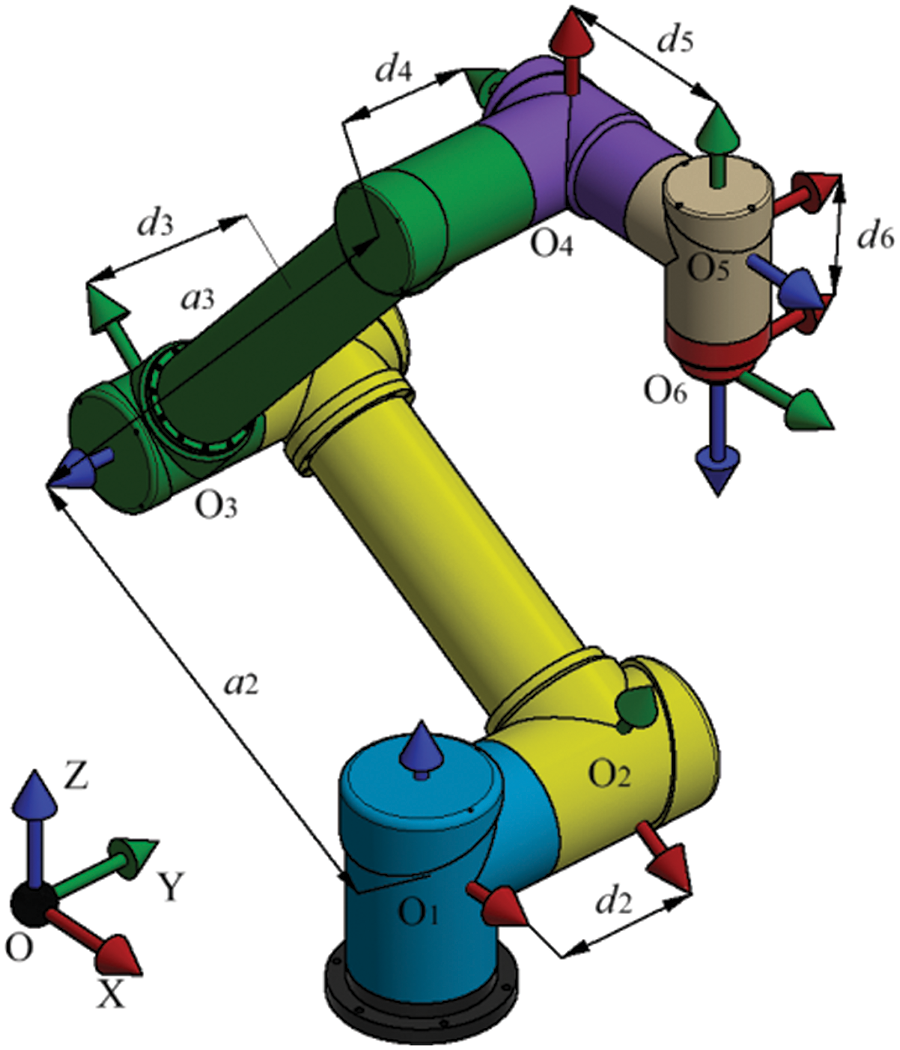
Figure 1: Manipulator structure and link coordinate systems

3  Methodology

3.1 Overview of RPP

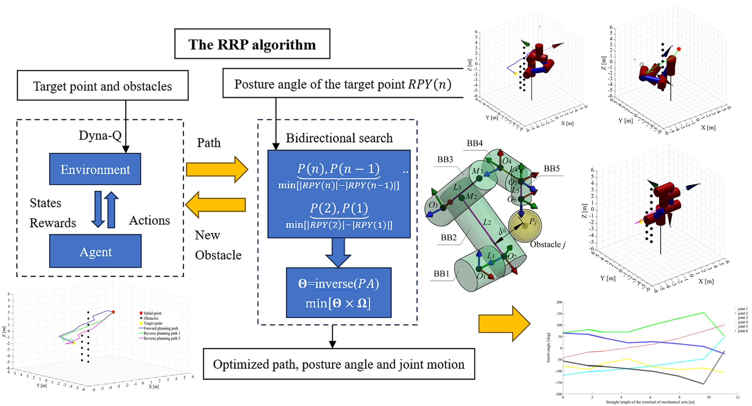
Considering the problem statement in Section 2, where the manipulator needs to meet a specific posture at the target position, this study is dedicated to the pursuit of reverse path planning within Cartesian space. The succession of positions and associated posture angles (PA values) derived through the path planning process necessitates conversion into the manipulator’s joint space via inverse kinematics. Subsequently, collision-free joint motions, characterized by minimal posture alteration and adherence to joint constraints, are chosen. Fig. 2 provides a visual representation of the foundational framework of the Reverse Path Planning (RPP) algorithm, with the ensuing steps delineated as follows:

1. In the first phase of RPP computation, this study employs the Dyna-Q algorithm from reinforcement learning to obtain a collision-free path composed of points for the manipulator’s end-effector. This path traverses from the target point to the starting point. The connection of these points with ordered straight-line segments culminates in the initial establishment of a collision-free path.

2. During the second phase of RPP computation, a bidirectional search algorithm is deployed in the opposite direction of the established collision-free path, utilizing the RPY posture angles of the target point. This process aims to determine the posture angles of all nodes while ensuring minimal posture increments between adjacent nodes.

3. The linear segment paths between adjacent nodes undergo discretization, resulting in a series of sub-paths. The complete PA information for these discrete path nodes comprises the positional value obtained in Step 1 for each node, along with the corresponding posture angle value from Step 2. These PA values are then applied in inverse kinematics to calculate all potential manipulator poses at each node while assessing whether any poses lead to collisions between the manipulator and obstacles. Nodes, where collisions are inevitable in all computed poses, are identified as new obstacles. In such a situation, the RPP algorithm reverts to Phase 1 to recommence the search for an obstacle-free path. Otherwise, RRP proceeds to select and optimize joint configurations from these inverse kinematic solutions.

4. The first phase of RPP is once again utilized to chart a new path from the target point to the starting point. This freshly computed path is optimized in terms of end-effector posture and joint configurations. Should the manipulator still confront unavoidable collisions, Steps 1 to 4 are reiterated.

5. In scenarios where all sub-paths from Step 3 exhibit no collisions with obstacles, an approach employing weighting coefficients is implemented. This methodology aids in the selection of joint configurations with minimal joint motion.

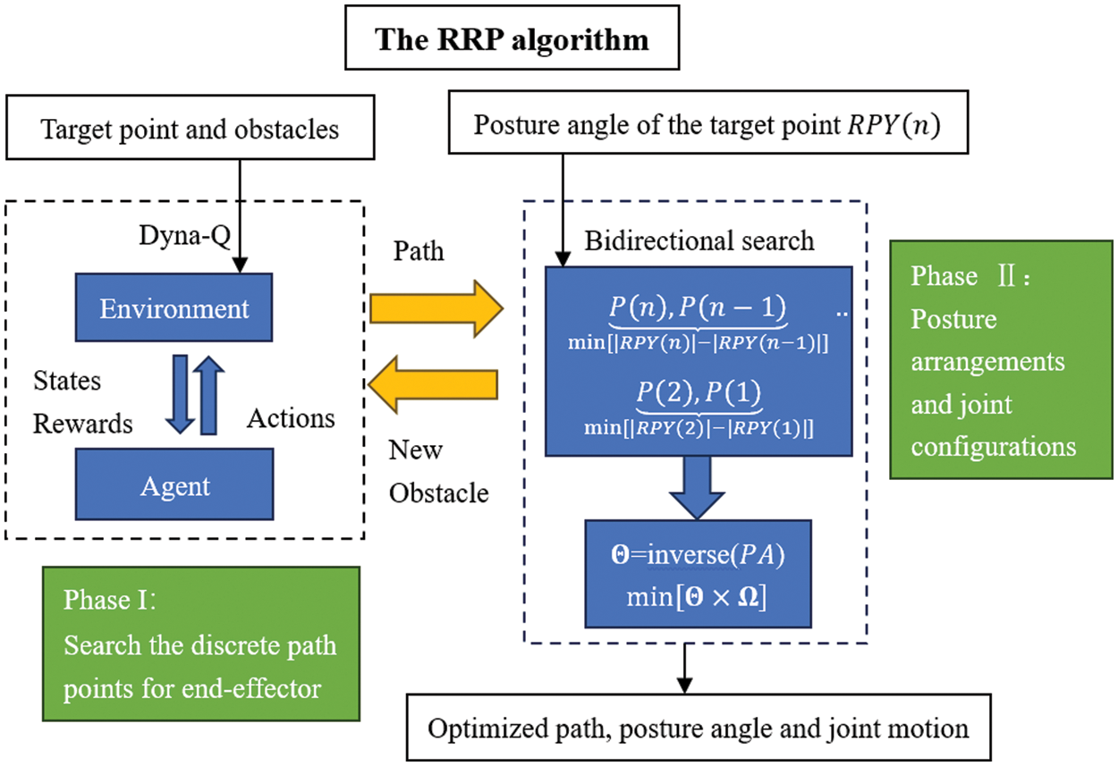
Figure 2: The framework of reverse path planning algorithm

3.2 Path Planning for Manipulator’s End-Effector

In the pursuit of attaining optimal collision-free paths, this study introduces reinforcement learning as the designated methodology, designating the manipulator’s end-effector as the intelligent agent. In tandem with this, the research acknowledges the uncertainties inherent in the environment and, as such, adopts a model-free exploration approach. This signifies that the intelligent agent engages directly with the environment, consistently acquiring real-time experiential data. This data forms the basis for learning and optimizing its collision-free path. Q-learning [25] stands out as an effective model-free strategy whose stability has been validated in both deterministic and non-deterministic Markov processes. Its learning rule is as follows:

Q(St,at)=(1−α)Q(St,at)+α(r+γmaxa⊆AQ(St+1,a))(2)

where α ∈ [0,1] represents the learning rate, γ ∈ (0, 1) is the discount factor, A is the set of actions, and r denotes the reward function. From Eq. (2), it is evident that estimating the action-value function Q(St,at) assists us in identifying the optimal action at for each state. When an appropriate reward function [26] is designed and algorithm convergence is ensured, the derived optimal strategy guides the agent toward the globally optimal path.

3.2.1 State Space

Indeed, the collision-free path is segmented into discrete nodes, systematically positioned between the initial point and the target point. Subsequently, each sub-path undergoes further discretization into a finite number of shorter line sub-paths. Through the utilization of the reinforcement learning agent tasked with locating these ordered nodes, the collision-free trajectory for the manipulator’s end-effector is derived. Consequently, the study defines the set of reachable node coordinates in the manipulator’s end-effector workspace as agent’s state space St:

St=[x(t),y(t),z(t)]

s.t.{xmin≤x(t)≤xmaxymin≤y(t)≤ymaxzmin≤z(t)≤zmax(3)

where x(t), y(t), and z(t) respectively represent the coordinates of the tth node along the X-axis, Y-axis, and Z-axis. xmin, xmax, ymin, ymax, zmin, and zmax correspond to the limits of the end-effector within the workspace. Additionally, to ascertain whether the manipulator’s end-effector collides with obstacles, the geometric center coordinates of m obstacles are defined in the manipulator’s workspace as follows:

Pj=[Xj,Yj,Zj]j∈1,2,3…m(4)

When St=Pj, it indicates that a collision has occurred between the manipulator’s end-effector and an obstacle.

3.2.2 Action Modeling and Selection

The collision-free path is constituted by a series of discrete nodes. In cases where the distance between adjacent nodes is determined by a random integer, it may result in an expansive defined action space, potentially leading to the issue of dimensionality curse. To address this issue and to facilitate a rapid validation of the proposed RPP algorithm, the study establishes the following provisions: 1. Coordinate values of the initial point, target point, intermediate nodes, and geometric centers of obstacles are all integers. 2. When the agent moves along any of the X, Y, or Z directions, the absolute value of the step increment is 1 unit length. Considering all the possible movement directions of the manipulator’s end-effector within the workspace, this study defines a discrete action set containing 26 actions:

A=[Δx,Δy,Δz,ΔxΔy,ΔxΔy¯,ΔxΔz,ΔxΔz¯,ΔyΔz,ΔyΔz¯,ΔxΔyΔz,ΔxΔyΔz¯,ΔxΔy¯Δz,ΔxΔy¯Δz¯,Δx¯,Δy¯,Δz¯,Δx¯Δy¯,Δx¯Δy,ΔxΔz¯,Δx¯Δz,ΔyΔz¯,Δy¯Δz,ΔxΔyΔz¯,ΔxΔy¯Δz,Δx¯ΔyΔz¯,Δx¯ΔyΔz](5)

where Δx, Δy, and Δz represent the unit step lengths along the positive directions of the world coordinate system’s X, Y, and Z axes for the manipulator’s end-effector. Δx¯, Δy¯, and Δz¯ correspond to unit step lengths in the negative directions. When the manipulator’s end-effector moves simultaneously along two or more coordinate axes, actions are defined using increments along multiple axes, such as ΔxΔy, ΔxΔz¯, and ΔxΔyΔz¯. The discrete set of actions, not confined to single-axis movement, contributes to obtaining the shortest collision-free path connected by a straight line.

3.2.3 Action Selection Strategy

The agent employs a greedy strategy to select an action at from the action set A in the current state. The study defines the greedy strategy πg as follows:

πg(at|St)={1Nnow0.1at=random(A)1−1Nnow0.1at=argmaxQ(St,at)atϵA(6)

where Nnow represents the current iteration sequence during RL iterative calculation. Eq. (6) ensures that the agent has a high probability of conducting random exploration in the early iterations. In contrast, toward the end of the iterations, there is a small probability of selecting actions other than the one with the maximum Q-value.

3.2.4 Reward Method

The reward function employed in this study encompasses four key components. Firstly, achieving the goal point is prioritized, with successful attainment yielding the highest reward of 200. Additionally, the proximity of the agent to the goal point is considered, where a decrease in the Euclidean distance between the current node and the target results in a reward increase of 1, indicating closer proximity. The occurrence of a collision and the breach of the reachable workspace are also factored into the reward function. This comprehensive approach to defining rewards ensures a balanced consideration of critical aspects in the path planning process, promoting effective and collision-free trajectory generation for the manipulator’s end-effector. Conversely, a reward decrease of 1 occurs if the distance increases. If the manipulator’s end-effector collides with obstacles or goes beyond the reachable workspace, the reward is assigned a negative value. The analytical description of the reward above function is as follows:

Rt(St,at,St+1)={+200if  S(t)=Stag+1if  d(St,Stag)≥d(St+1,Stag)−1if  d(St,Stag)≤d(St+1,Stag)−100if  St+1=Pj  j∈1,2,3…m−5if{xmin≤x(t)≤xmaxymin≤y(t)≤ymaxzmin≤z(t)≤zmax(7)

where d(St,Stag) denotes Euclidean distance between the current position and the goal position, defined as follows:

d(St,Stag)=(xt−xtag)2+(yt−ytag)2+(zt−ztag)2(8)

3.2.5 Dyna-Q Method

In this study, the workspace of the manipulator’s end-effector is designated as the state space, effectively discretizing and determining the environment for path planning. To expedite the learning process of reinforcement learning (RL), this study enhances the standard Q-learning framework by introducing a Dyna-Q framework. This modification involves the creation of an environment model that stores past experiences, facilitating more efficient and effective learning in the path planning process. The virtual samples generated by this model can serve as learning samples for the iterative update of Q-values [27,28], thus accelerating algorithm convergence within a finite number of iterations. As depicted in Fig. 3, under the Dyna-Q framework, during the manipulator’s end-effector seeking its target position, each interaction with the actual environment yields direct real experience [St,at,St+1,Rt] that is used to update Q-values. Simultaneously, the intelligent agent constructs a model (St,at) concerning an assumed deterministic environment within the system. Interaction between the agent and these models results in simulated experience [St,at′,St+1′,Rt′], and the simulated experiences gained from these models assist in updating Q-values. In the Dyna-Q framework, every action undertaken by the agent results in updating Q-values once based on actual experience and additionally updating Q-values m times based on simulated experience from the environment model. Consequently, Q-values are updated nm times within n times iterations. Therefore, within a finite number of iterations, the intelligent agent can enhance the speed of optimal path planning without running into non-convergence issues stemming from insufficient iteration counts.

Figure 3: The framework of Dyna-Q

3.3 Collision Detection and Multi-Objective Optimization in Reverse Path Planning

3.3.1 Collision Detection

Bounding volume technology stands as a classic technique in manipulator collision detection. This technology encompasses well-known approaches such as Aligned Axis Bounding Box (AABB), Oriented Bounding Box (OBB), and Discrete Orientation Polytope (DOP) [29], all of which contribute to reducing computational demands. This paper introduces a novel approach using DH parameters of the robot to model cylindrical bounding volumes, facilitating accelerated collision detection.

Suppose the coordinates of the joint origins of manipulator links Li and Li+1 relative to the base origin are respectively denoted as Oi(Xi(t),Yi(t),Zi(t)) and Oi+1(Xi+1(t),Yi+1(t),Zi+1(t)). In accordance with the DH parameters of link Li, the study defines the centerline of its cylindrical bounding block BBi. Two scenarios are illustrated as follows:

1. When ai=0 in DH parameters of link i+1, the centerline of the cylindrical bounding block BBi for link i is represented by OiOi+1→, and the length of the link is denoted as |OiOi+1|. This case is illustrated by links 1, 4, and 5 in Fig. 1.

2. When ai≠0 in DH parameters of link i+1, the centerline of the cylindrical bounding block BBi for link i aligns with the perpendicular line between the Z axes of adjacent coordinate systems Zi and Zi+1. If the foot of this perpendicular line is designated as Mi, the centerline direction becomes OiMi→, and the length of the link is given by |ai|. This scenario is exemplified by links 2 and 3 in Fig. 1.

After obtaining the centerlines for all cylindrical bounding blocks of the individual links, the overall cylindrical envelope of the manipulator can be defined by taking a radius slightly larger than the radial dimension ri of each link. Since the manipulator’s base remains fixed and does not require enveloping, the cylindrical envelopes for a six-axis manipulator are ultimately determined as [BB1,BB2,BB3,BB4,BB5], as depicted in Fig. 4.

Figure 4: The cylinder bounding box of robot

Subsequently, this study employs sphere-bound volumes to simplify obstacles. The jth obstacle’s geometric center coordinates are denoted as Pj(Xj,Yj,Zj), and the corresponding bounding radius is Rj. During collision detection, it treats the set of points along the centerline direction of each bounding block BBi, within the length range of the link, as collision monitoring points. Referring to Fig. 4, the cylinder and the sphere are tangential when the manipulator is in direct contact with an obstacle. At this point, the distance dij between the sphere and the cylinder is defined as follows:

dij={k|OiOi+1→×OiPj→||OiOi+1→|ai=0k|OiMi→×OiPj→||OiMi→|ai≠0(9)

Here, the symbol '×' represents the cross product. Due to the actual length of the manipulator links being greater than the length of their cylindrical bounding block centerlines, Eq. (9) introduces a safety factor k greater than 1 to perform length correction. When dij≤(ri+Rj), the link collides with the obstacle, necessitating adjustments to the manipulator’s pose and joint angles. Conversely, when dij>(ri+Rj), the manipulator does not collide with the obstacle.

During autonomous path planning of a six-axis manipulator, the RPP algorithm derives the manipulator’s various joint angles [θ1,θ2,θ3,θ4,θ5,θ6] based on the end-effector’s posture. Subsequently, these angles are applied to the manipulator’s DH mathematical model to obtain the values of the centerlines [O1O2→,O2M2→,O3M3→,O4O5→,O5O6→] of the cylindrical bounding block collection [BB1,BB2,BB3,BB4,BB5]. By employing Eq. (9), the distances between each manipulator link and the geometric centers [P1,P2,⋯,Pn] of the m obstacles are sequentially calculated, allowing for the swift determination of whether the manipulator collides with any obstacles. This approach simplifies the collision detection process.

3.3.2 End-Effector’s Posture Optimization

The collision-free paths obtained via reinforcement learning algorithms offer an initial outline of the manipulator end-effector’s coordinate trajectory, but do not precisely define its specific posture. In subsequent research, this study endeavors to refine the Reverse Path Planning (RPP) algorithm, specifically targeting the enhancement of end-effector posture smoothness and minimizing joint movement. This refinement aims to optimize the manipulator’s autonomous obstacle avoidance process, ensuring a seamless and efficient operational workflow.

As outlined in the problem description in Section 2, the posture angles rx(t), ry(t), and rz(t) at non target points are treated as redundant variables since they are not assigned. Starting from the goal pose with given posture angles, planning posture angles for all discrete positions along the collision-free path in the reverse direction would incur substantial computational overhead. To circumvent this, this research discretizes the collision-free path into a sequence of short sub-paths segmented by nodes. The paper aims to optimize the manipulator’s end-effector’s kinematic performance by minimizing the adjacent nodes’ absolute angular increments. In this study, the interval (−π,π] is divided into 2n equal parts,and they are employed as optional angular increments Δrx, Δry, and Δrz for the end-effector along the X, Y, and Z axes, respectively:

Δrx,y,z=πin,  n∈N∗,  i=0,1,−1,2,−2⋯(n−1),−(n−1),n(10)

The values of Δrx, Δry, and Δrz in Eq. (10) each have 2n possible choices. As a result, there are a total of 8n3 potential arrangements for the postures of adjacent nodes. Arranging these 8n3 combinations according to a certain pattern helps us prioritize the combination with the smallest absolute increment of posture angle. Upon rearranging Eq. (10) in an ascending pattern, Δrx,y,z = [−π(n−1)n…,−πn,0,πn,…,π(n−1)n,π] is obtained. In this set, the 0 elements signify that the current angular increment is 0, and the elements with equal absolute increments are symmetrically distributed on both sides of the 0 elements. Utilizing this arrangement approach, a bidirectional search method successively determines the minimum posture for each node along the collision-free path, proceeding from the target point to the initial point.

The combinations of orientations’ increments in the X, Y, and Z directions are arranged using ix, iy, and iz. Subsequently, by letting M=|ix|+|iy|+|iz|, the aforementioned 8n3 combinations are stored based on M-values as sequence numbers. Given that the values of M range from integers 0∼3n, there are 3n+1 possible values for the absolute angular increments between adjacent node orientations, including the case with a 0 increment. On the basis of the above, to differentiate the priority of combinations stored within the same region, the study established the following three rules: 1. Priority is given to single-axis rotation over double-axis rotation and then triple-axis rotation; 2. In the event of an equal number of rotation axes, the selection of rotation axes follows the order of priority: +X, −X, +Y, −Y, +Z, −Z, +X+Y, +X−Y, −X+Y, −X−Y, +X+Z, +X−Z, −X−Z, …; 3. When there is more than one rotation angle and the rotation axes are the same, the posture angles are randomly chosen.

Based on the description mentioned above, if n=4 in Eq. (10), and assuming that the feasible combinations for ix, iy, and iz which satisfy path planning for the manipulator are [1,0,−2], [3,0,0], [0,3,0], and [2,0,−1], the corresponding posture angle increments should be [π4,0,−π2], [3π4,0,0], [0,3π4,0], and [π2,0,−π4]. As the sum of |ix|+|iy|+|iz| for these combinations are all 3, they are stored in the third region. Following Rule 1, the algorithm prioritizes the selection of [3π4,0,0] and [0,3π4,0] as the posture angle increments for the current node. If both inverse kinematics solutions of these two postures result in a collision between the manipulator and the obstacles, according to Rules 2 and 3, randomly select one of the increment combinations [π4,0,−π2] and [π2,0,−π4] as the posture angle increment of the current node, and continue to test whether the manipulator collides with the obstacles under these two postures. A detailed description of the bidirectional search algorithm is integrated into Algorithm 1.

3.3.3 Joint Motion Optimization

The steps mentioned above have guided the manipulator’s end-effector in achieving a collision-free path while ensuring smooth posture angles at the path nodes. These obtained path points’ positional and PA values can be used to deduce the manipulator’s various joint angles. The manipulator’s kinematic inverse solutions must adhere to Pieper criteria [30]. On this basis, according to reference [31], a 6R-type manipulator with a given posture can obtain eight kinematic inverse solutions. Among these solutions, the study first eliminates those that violate joint limits, are singular, or collide with obstacles. Subsequently, considering the rated power of each joint in the manipulator from the remaining solutions, the study designs weighting coefficients Ω=[ω1,ω2,ω3,ω4,ω5,ω6] to filter out inverse solutions with minimal joint configurations for high-power joints. These selected configurations serve as the final joint configurations.

Assuming at Node t1, the manipulator’s joint angles are Θ(t1)=[θ1(t1),θ2(t1),θ3(t1),θ4(t1), θ4(t1),θ5(t1),θ6(t1)] and at the adjacent node t2, the position and posture are PA(t2)=[x(t2),y(t2), y(t2),z(t2),rx(t2),ry(t2),rz(t2)]. The feasible joint configurations for the manipulator are Θ(t2)={Θ1(t2),Θ2(t2),Θ3(t2),Θ4(t2),Θ5(t2),Θ6(t2),Θ7(t2),Θ8(t2)}. In this study, Eq. (11) is used to filter out the Eth set of solutions Θ(E) that satisfies the constraint conditions.

E=argmin{|Θe(t2)−Θ(t1)|×ΩT}e=1,2⋯

s.t.{Θmin≤Θe(t2)≤Θmax|J(Θe(t2))|>εiscols(Θe(t2))=0(11)

where Θmin and Θmax represent the lower and upper joint limits, respectively. The kinematic Jacobian matrix of the robot with configuration Θe(t2) is denoted as J(Θe(t2)), and its determinant should exceed a specified value of ε to prevent singularities. The binary function iscols is used to ascertain whether the manipulator’s links and joints collide with obstacles. Assuming there are l inverse solutions of the manipulator joints that satisfy the three constraints in Eq. (11), denoted as Θ(t2)={Θ1(t2),Θ2(t2),…,Θl(t2)}, the study selects the Eth group solution Θ(E) from these that minimizes the weighted sum of joint angle increments as the final joint configurations.

In the RPP algorithm, the optimization processes for the manipulator’s end-effector orientation and joint motion are transformed into a graphical representation, as depicted in Fig. 5. The pseudocode summarizing this process is provided in Algorithm 1. In Algorithm 1, Pm, D0, Dq, ΔRPY, RPY(t), and other boldface variables are all matrix sets representing n rows and 3 columns.

Figure 5: Schematic diagram of posture and joint motion optimization in the RPP method

4  Experiment Results

4.1 Simulation Parameters

The D-H parameters used by the six-DOF manipulator arm are shown in Table 1. The other simulation parameters are as follows:

The weighting coefficients: Ω=[1,1.2,1.2,0.6,0.2,0.1]; The radius of spherical obstacles: Rj=0.3 m; The radius of the manipulator’s cylindrical bounding box: ri=0.5 m; The learning rate: α=0.05; The discount factor: γ=0.9; The iteration times of RL in path planning: NQ=104; The number of times Dyn-Q updates the Q-value based on the simulation experience of the model in each iteration of the RL calculation: Nd=80; The incremental division value of posture angle: 45∘; Coordinate of the initial point: [0, −2, 4]; Coordinate of the target point 1: [−1, 3, −2]; Coordinate of the target point 2: [0, 3, −2]; Geometric center coordinates of Obstacle 1: [0, 2, −5; 0, 2, −4; 0, 2, −3; 0, 2, −2; 0, 2, −1; 0, 2, 0; 0, 2, 1; 0, 2, 2; 0, 2, 3; 0, 3, −5; 0, 3, −4; 0, 3, −3; 0, 3, −2; 0, 3, −1]; Geometric center coordinates of Obstacle 2: [0, 2, 0; 0, 2, 2; 0, 2, 1; 0, 1, −1; 0, 2, −1; 0, 1, 1; 0, 1, 2].

All computations in this paper have been performed on a 2.5 GHz. Intel Core (TM) i5-7300HQ processor with 16 GB of RAM.

4.2 The Iterative Process of RL

The number of nodes of all the episodes in the first learning process of the RPP algorithm are shown in Fig. 6. At the beginning of the iteration, to update Q-values more frequently, Dyn-Q searches more nodes than Q-learning. Since the 700-th episode, the number of nodes obtained by Dyn-Q began to decrease gradually. After the 4000-th episode, the algorithm converges basically, and the number of path nodes is also within the range of 8–10 stably. In Fig. 6, it is evident that the iteration curve of Dyn-Q significantly outperforms that of Q-learning. Notably, the iteration time required for Q-learning is 1853 s, whereas the iteration time for Dyn-Q stands at a notably lower 1531 s. This iterative computation process serves as compelling evidence that Dyn-Q exhibits a swifter convergence rate compared to Q-learning. Consequently, this accelerated convergence ensures that the Reverse Path Planning (RPP) algorithm can expeditiously generate an initial collision-free path, contributing to enhanced efficiency in path planning.

Figure 6: Learning process of Q learning and Dyn-Q

4.3 The Results of RPP

For comparison, the forward planning (FP) method [32] without additional bidirectional search and weighting coefficients is used to obtain the collision-free path. The blue line in Fig. 7a shows the result. All the nodes’ coordinates and posture angles are arranged in Table 2.

Figure 7: The path of the end-effector of the manipulator in different situations

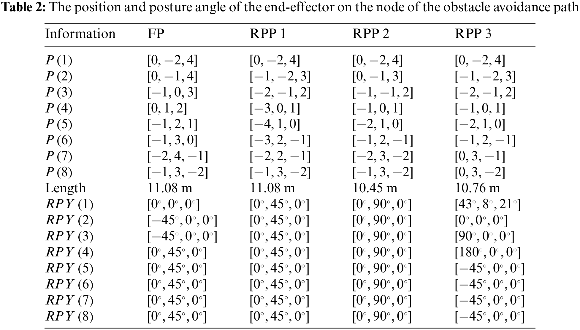
The collision-free of the manipulator in Fig. 7a includes 8 nodes and 7 linear segment sub-paths. The closer a node is to the target point, the shorter the distance between it and the target point. For example, the distances between nodes 1, 2, and 3 and the target point are 7.874 m, 7.28 m, and 5.83 m, respectively. The effectiveness of the reward function defined in Eq. (7) is clearly demonstrated in its capacity to discern the optimal action for each state. This ensures a gradual approach of the manipulator towards the target point, ultimately resulting in the determination of the shortest path. However, owing to the inherent nature of forward planning, wherein calculations proceed from the starting point to the target point, there arises a limitation. Specifically, the manipulator’s end-effector encounters difficulty in achieving effective control precisely at the target point. Regrettably, this circumstance does not align with the specific task requirements detailed in Section 2. Furthermore, the last 8 data in the first column of Table 2 indicate that the posture of the end-effector fluctuates to a certain extent between adjacent nodes, with a posture angle variation of 90∘. Moreover, during the motion of the manipulator, the X and Y axes of the end coordinate system are used for posture changes, which does not comply with the rule in 3.3.2 that the rotation axis should be selected in the order of X, Y, and Z axes for the same absolute increment of posture angle. In this collision-free path, the motion of joints 1 to 6 is shown in Fig. 8a, with motion ranges of 171.6∘,91.4∘,135.3∘,104.9∘,208.9∘, and 157.5∘, respectively. Although all joint angles are within their limits, the first three high-power joints have relatively large motion ranges, with an average angle change of 132.8∘. Therefore, while forward planning can provide a collision-free path, the end-effector’s posture and joint angle changes do not meet task requirements 1, 2 and 3 in Section 2.

Figure 8: The results of the joint angles in different situation

To verify the effectiveness of the proposed RPP algorithm, tests were carried out in a scenario in which the posture angle of the target point is the same as the FP method. The green line in Fig. 7a represents the path obtained using the RPP algorithm. Due to the re-planning of the terminal posture Angle, the green line does not coincide with the blue line. The calculations reveal that both the RPP and FP paths share an identical total length, measuring precisely 11.08 m. This observation underscores that the node coordinates for both RPP and FP exhibit a congruent distribution pattern, progressively converging towards the target point. Furthermore, the last eight data points in the second column of Table 2 show that due to the addition of the bidirectional search method, the posture angle of the manipulator’s end-effector is always maintained at [0∘,45∘,0∘] at each node, which is clearly a very smooth motion process. The joint motion of the manipulator during obstacle avoidance is shown in Fig. 8b, with the range of angle changes from joint 1 to joint 6 being 142.9∘,89.6∘,59.9∘,101.7∘,164.5∘ and 142.3∘, respectively. Due to the addition of weighting coefficients, the range of joint 1~3 high-power joints are significantly reduced compared to the FP experiment. Particularly, joint 3 has nearly halved its range. The average angular change for the first three joints is 97.5∘, representing a 26.58% reduction compared to forward planning.

To further test the RPP algorithm, the obstacle and target positions were kept unchanged, and the posture angle of the target point was set to [0∘,90∘,0∘]. The RPP algorithm was once applied to plan the collision-free path. The pink line in Fig. 7a represents the collision-free path obtained in this second experiment, with a total length of 10.45 m, almost the same as the previous two experiments. In Fig. 7a, the blue, green, and pink paths gradually descend in the Z-direction, which is because, in the last two experiments, the end-effector rotated around the Y-axis by 45°and 90°, respectively, resulting in a decrease in the position and posture of the manipulator in sequence. The last eight data points in the third column of Table 2 indicate that the end-effector’s posture angle remains constant at [0∘,90∘,0∘] throughout the collision-free path. The joint motion of the manipulator is shown in Fig. 8c, with angular ranges specified for joints 1 to 6 as 132.7∘,113.3∘,81.2∘,88.4∘,132.8∘, and 0∘, respectively, and the average Angle variation range of the first three joints is 109.1°. Compared to experiment two, the motion range for the first three joints has not changed significantly. Relative to the FP method, the range of joint motion has been reduced by 17.85%. The fourth and fifth joints have significantly smaller ranges compared to experiment one, and the sixth joint always remains stationary.

The above three experiments demonstrate that for a manipulator with a known target point position and posture, the proposed RPP algorithm while ensuring a collision-free path, exhibits three significant advantages: 1. Ensuring the shortest straight-line path length; 2. Smooth the end-effector’s posture; 3. Reduce the motion of high-power joints.

In order to validate the RPP algorithm proposed in this paper more generally, the positions of the target point and obstacles are changed, and the posture angle of the target point is also randomly set to [43∘,8∘,21∘].

The collision-free path obtained by the RPP algorithm is shown in cyan in Fig. 7b, with the coordinates of path nodes and posture angles compiled in the fourth column of Table 2. Upon comparison, the total length of this collision-free path is approximately the same as the three paths in Fig. 7a, and the change rule of node coordinates aligns with the previous three cases. The joint motion for collision-free of the manipulator is shown in Fig. 8d. The angle variation range of joint 1 to joint 6 is 111.3∘,113.8∘,283.6∘,259.5∘,45.1∘, and 341.2∘, respectively. Compared to the previous three experiments, when the end-effector transitions from node 4’s posture angle [180∘,0∘,0∘] to node 5’s posture angle [180∘,0∘,0∘], large movements occur for joint 3. The reason is that in this experimental scenario, the obstacles are closer to the manipulator, and the target point is completely hidden behind the obstacles. This results in a smaller avoidance space along the Y-axis between the manipulator and the obstacles. Joint 3 needs to rotate significantly in the negative direction to move the three links articulated with it to the avoidance space beneath the obstacles. The change pattern of the end-effector’s posture angles listed in Table 2 adheres to the rules of the bidirectional search method outlined in Section 3, prioritizing single-axis changes when the absolute increment in posture angles at adjacent nodes is the same and following the order of X, Y, and Z for assignment. For the collision-free path after node 5, since the manipulator already has sufficient avoidance space, posture angles remain unchanged from node 5 to node 8, corresponding to joint ranges for joints 1 to 3 less than 40°. The manipulator’s motion is smooth throughout this process.

In the conclusive phase, Matlab’s Robotics Toolbox was employed to visually represent the collision-free motion of the 6-degree-of-freedom (6-DOF) manipulator across the four experiments, as indicated in Fig. 9. All the figures labeled (a) in Fig. 9 depict the manipulator’s initial pose, while those labeled (b) and (c) represent the manipulator’s poses at intermediate nodes, and (d) show the manipulator’s target pose. Throughout the process, the end-effector strictly follows the obstacle avoidance path shown in Fig. 7, successfully avoiding obstacles and safely reaching the target point. In Figs. 9b to 9d, while the manipulator is engaged in obstacle avoidance, the end-effector undergoes minimal changes in posture, and it arrives at the target location in the specified posture.

Figure 9: The action of the 6-DOF manipulator in different situations

The sequential execution times for the three RPP experiments mentioned above were 1840, 1810, and 4426 s, respectively. Notably, Experiment 3 exhibited the longest computation time, while the computation times for the first two experiments were relatively close. Further investigation revealed that Experiment 3 involved three alternations between two complete phases of the RPP algorithm, whereas the first two experiments included only one alternation between two complete phases. This observation suggests that while RPP can identify the shortest path within the first phase, it cannot guarantee the acquisition of suitable posture angles and feasible kinematic solutions in the second phase. Consequently, the computational complexity of the RPP algorithm is predominantly determined by the second phase. In Experiment 3, the cramped space between obstacles and the manipulator compelled the RPP algorithm to explore all conceivable postures during the initial two complete iterations. However, none of these attempts proved successful in avoiding collisions with obstacles. Consequently, in cases where, during the second phase of RPP computation, all posture angles configured by the algorithm lead to collisions between the manipulator and obstacles, the RPP algorithm fails to converge. Furthermore, when the target point falls outside the reachable workspace of the manipulator, the RPP algorithm also fails to converge.

5  Conclusion

This paper addresses the intricate task of collision-free path planning for industrial manipulators, which encompasses the optimization of path, end-effector posture, and joint motion. To account for real-world scenarios, the study introduces the Reverse Path Planning (RPP) algorithm, which effectively devises collision-free paths originating from the target point and extending back to the initial point. By leveraging reinforcement learning, a sequence of nodes is obtained and subsequently connected to establish a collision-free trajectory. To enhance path search efficiency, the Q-learning approach is augmented as Dyn-Q. Additionally, collision detection leverages the Denavit-Hartenberg (DH) parameters of the manipulator, ultimately yielding a collision-free path through reverse planning. Furthermore, in the process of planning end-effector posture and joint motion, the utilization of bidirectional search and weighted coefficient methods proves instrumental in achieving significant improvements in the smoothness of both end-effector posture and joint movements. The most significant contribution of this study is the realization of multi-objective optimization in the path planning process, particularly for MDOF manipulators that demand precise posture adjustments at the target position.

It is essential to acknowledge that, to mitigate computational complexity in this study, we designated node coordinates, target point coordinates, and obstacle center coordinates as integers. In practical engineering scenarios, there exists the potential to refine measurement units and augment positioning precision following specific application requirements. Additionally, polynomial or B-spline fitting techniques can be employed to further smooth the obstacle avoidance paths. We hope to implement these in future work.

Acknowledgement: The authors wish to express their appreciation to the reviewers for their valuable suggestions that enhanced the paper’s quality. We also sincerely appreciate the editors for their patience, supportive reminders, and dedicated efforts in editing the manuscript. We extend heartfelt thanks to all the authors for contributing to this paper.

Funding Statement: This research work is supported by the National Natural Science Foundation of China under Grant No. 62001199; Fujian Province Nature Science Foundation under Grant No. 2023J01925.

Author Contributions: The authors confirm contribution to the paper as follows: study conception and design: Zhiwei Lin; data collection: Zhiwei Lin, Jianmei Jiang; analysis and interpretation of results: Zhiwei Lin, Hui Wang, Tianding Chen; manuscript writing: Zhiwei Lin, Hui Wang, Tianding Chen. manuscript review and editing: Yingtao Jiang, Yingpin Chen. All authors reviewed the results and approved the final version of the manuscript.

Availability of Data and Materials: The manuscript included all required data and implementing information.

Conflicts of Interest: The authors declare that they have no conflicts of interest to report regarding the present study.

References

1. Nagatani, K., Fujino, Y. (2019). Research and development on robotic technologies for infrastructure maintenance. Journal of Robotics and Mechatronics, 31(6), 744–751. [Google Scholar]

2. Fang, H. C., Ong, S. K., Nee, A. Y. C. (2016). Robot path planning optimization for welding complex joints. The International Journal of Advanced Manufacturing Technology, 90(9), 3829–3839. [Google Scholar]

3. Lu, Y. A., Tang, K., Wang, C. Y. (2021). Collision-free and smooth joint motion planning for six-axis industrial robots by redundancy optimization. Robotics and Computer-Integrated Manufacturing, 68, 91–107. [Google Scholar]

4. Wei, Y. Z., Gu, K. F., Cui, X. J., Hao, C. Z., Wang, H. G. et al. (2016). Strategies for feet massage robot to position the pelma acupoints with model predictive and real-time optimization. International Journal of Control, 14(2), 628–636. [Google Scholar]

5. Li, Y., Liu, K. P. (2019). Two-degree-of-freedom manipulator path planning based on zeroing neural network. 2019 IEEE 7th International Conference on Computer Science Communication and Network Security, pp. 1–8. Dalian, China. [Google Scholar]

6. Secil, S., Ozkan, M. (2023). A collision-free path planning method for industrial robot manipulators considering safe human-robot interaction. Intelligent Service Robotics, 16(3), 323–359. [Google Scholar]

7. Dijkstra, E. W. (1959). A note on two problems in connexion with graphs. Numerische Mathematik, 1, 269–271. [Google Scholar]

8. Hart, P. E., Nilsson, N. J., Raphael, B. (1968). A formal basis for the heuristic determination of minimum cost paths. IEEE Transactions on Systems Science and Cybernetics, 4(2), 100–107. [Google Scholar]

9. Fu, B., Chen, L., Zhou, Y. T., Zheng, D., Wei, Z. Q. et al. (2018). An improved A* algorithm for the industrial robot path planning with high success rate and short length. Robotics and Autonomous Systems, 106, 26–37. [Google Scholar]

10. Persson, S. M., Sharf, I. (2014). Sampling-based A* algorithm for robot path-planning. The International Journal of Robot Res, 33(13), 1683–1708. [Google Scholar]

11. Macenski, S., Moore, T., Lu, D. V., Merzlyakov, A., Ferguson, M. (2023). From the desks of ROS maintainers: A survey of modern & capable mobile robotics algorithms in the robot operating system 2. Robotics and Autonomous Systems, 168, 1–12. [Google Scholar]

12. Khatib, O. (1986). Real-time obstacle avoidance for manipulators and mobile robots. The International Journal of Robotics Research, 5(1), 90–98. [Google Scholar]

13. Wang, W. R., Zhu, M. C., Wang, X. M., He, S., He, J. P. et al. (2018). An improved artificial potential field method of trajectory planning and obstacle avoidance for redundant manipulators. International Journal of Advanced Robotic Systems, 15(5), 1–13. [Google Scholar]

14. Xu, T. Y., Zhou, H. B., Tan, S. X., Li, Z. Q., Ju, X. (2021). Mechanical arm obstacle avoidance path planning based on improved artificial potential field method. Industrial Robot, 49(2), 271–279. [Google Scholar]

15. Kavraki, L. E., Svestka, P., Latombe, J. C., Overmars, M. H. (1996). Probabilistic roadmaps for path planning in high-dimensional configuration spaces. IEEE Transactions on Robotics and Automation, 12(4), 566–580. [Google Scholar]

16. Lavalle, S. M. (1998). Rapidly-exporing random trees: A new tool for path planning. In: Algorithmic and computational robotics new direction, pp. 293–308. USA: Tech Science Press. [Google Scholar]

17. Gao, Q. Y., Yuan, Q. N., Sun, Y., Xu, L. Y. (2023). Path planning algorithm of robot arm based on improved RRT* and BP neural network algorithm. Journal of King Saud University—Computer and Information Sciences, 35(8), 1–14. [Google Scholar]

18. Qureshi, A. H., Ayaz, Y. (2016). Potential functions based sampling heuristic for optimal path planning. Autonomous Robots, 6, 1079–1093. [Google Scholar]

19. Kumar, A., Raj, R., Kumar, A., Verma, B. (2023). Design of a novel mixed interval type-2 fuzzy logic controller for 2-DOF robot manipulator with payload. Engineering Applications of Artificial Intelligence, 123, 1–15. [Google Scholar]

20. Izquierdo, R. C., Cukla, A. R., Lorini, F. J., Perondi, E. A. (2023). Optimal two-step collision-free trajectory planning for cylindrical robot using particle swarm optimization. Journal of Intelligent & Robotic Systems, 108(3), 1–15. [Google Scholar]

21. Wang, S. X., Wang, W. J., Cao, Y. T., Luo, Y., Wang, X. H. (2023). Obstacle avoidance path planning of 7-DOF redundant manipulator based on improved ant colony optimization. Recent Patents on Mechanical Engineering, 16(3), 177–187. [Google Scholar]

22. Zhong, J., Wang, T., Cheng, L. L. (2022). Collision-free path planning for welding manipulator via hybrid algorithm of deep reinforcement learning and inverse kinematics. Complex and Intelligent Systems, 8, 1899–1912. [Google Scholar]

23. Park, K. W., Kim, M. S., Kim, J. S., Park, J. H. (2022). Path planning for multi-arm manipulators using soft actor-critic algorithm with position prediction of moving obstacles via LSTM. Applied Sciences, 12(19), 9837–9857. [Google Scholar]

24. Yu, J. X., Arab, A., Yi, J. G., Pei, X. F., Guo, X. X. (2022). Hierarchical framework integrating rapidly-exploring random tree with deep reinforcement learning for autonomous vehicle. Applied Intelligence, 53(13), 16473–16486. [Google Scholar]

25. Watkins, C. J. C. H., Dayan, P. (1992). Technical note: Q-learning. Machine Learning, 8, 279–292. [Google Scholar]

26. Lin, Z. W., Chen, T. D., Jiang, Y. T., Wang, H., Lin, S. Q. et al. (2023). B-Spline-based curve fitting to cam pitch curve using reinforcement learning. Intelligent Automation & Soft Computing, 36(2), 2145–2164. https://doi.org/10.32604/iasc.2023.035555 [Google Scholar] [CrossRef]

27. Hwang, K. S., Jiang, W. C., Chen, Y. J. (2015). Model learning and knowledge sharing for a multiagent system with Dyna-Q learning. IEEE Transactions Cybernetics, 45(5), 964–976. [Google Scholar]

28. Hwang, K. S., Jiang, W. C., Chen, Y. J., Hwang, I. (2017). Model learning for multistep backward prediction in Dyna-Q learning. IEEE Transactions on Systems Man and Cybernetics Systems, 48(9), 1470–1481. [Google Scholar]

29. Aalhasan, A., Tang, X. Q., Song, B. (2016). Collision detection and trajectory planning for palletizing robots based OBB. Indonesian Journal of Electrical Engineering and Computer Science, 1(1), 109–118. [Google Scholar]

30. Pieper, D. L. (1968). The kinematics of manipulators under computer control (Ph.D. Thesis). University of Stanford, USA. [Google Scholar]

31. Ananthanarayanan, H., Ordóñez, R. (2015). Real-time inverse kinematics of (2n+1) DOF hyper-redundant manipulator arm via a combined numerical and analytical approach. Mechanism and Machine Theory, 91, 209–226. [Google Scholar]

32. Jia, Y. S., Li, Y. C., Xin, B., Chen, C. L. (2020). Path planning with autonomous obstacle avoidance using reinforcement learning for six-axis arms. 2020 IEEE International Conference on Networking, Sensing and Control, pp. 1–6. Nanjing, China. [Google Scholar]