
 Submit a Paper
 Propose a Special lssue
 Open Access
ARTICLE

A Study on the Transmission Dynamics of the Omicron Variant of COVID-19 Using Nonlinear Mathematical Models
1 Department of Mathematics, Periyar University, Salem, Tamilnadu, 636011, India
2 Faculty of Engineering and Natural Sciences, Istanbul Okan University, Istanbul, Turkey
3 Department of Mathematics, College of Science and Humanities in Alkharj, Prince Sattam Bin Abdulaziz University, Alkharj, 11942, Saudi Arabia
4 Department of Applied Mathematics, Faculty of Mathematics, Statistics and Computer Science, University of Tabriz, Tabriz, Iran
* Corresponding Author: Pushpendra Kumar. Email:
(This article belongs to the Special Issue: Recent Developments on Computational Biology-I)
Computer Modeling in Engineering & Sciences 2024, 139(3), 2265-2287. https://doi.org/10.32604/cmes.2023.030286
Received 29 March 2023; Accepted 26 July 2023; Issue published 11 March 2024
 View Full Text
 Download PDF
Abstract
This research examines the transmission dynamics of the Omicron variant of COVID-19 using SEIQIcRVW and SQIRV models, considering the delay in converting susceptible individuals into infected ones. The significant delays eventually resulted in the pandemic’s containment. To ensure the safety of the host population, this concept integrates quarantine and the COVID-19 vaccine. We investigate the stability of the proposed models. The fundamental reproduction number influences stability conditions. According to our findings, asymptomatic cases considerably impact the prevalence of Omicron infection in the community. The real data of the Omicron variant from Chennai, Tamil Nadu, India, is used to validate the outputs.Keywords
Since COVID-19 is a newly discovered virus, little is known about how it spreads. As a result, health authorities must thoroughly understand the incubation and recovery periods to implement more efficient quarantine procedures for those suspected of carrying the virus. As of November 24, 2021, Omicron has been found in countries, and it continues to be the most popular variant all over the world. The transmission dynamics and the potential roles of various intervention strategies have been better understood by recent COVID-19 studies [1–7]. These methodologies incorporate relief and concealment to dial back the spread of the pandemic, decreasing pinnacle medical care to safeguard the people who are most in danger from contaminations, lessening the number of infective cases to a low level, implementing lockdown to a district of exceptionally infective cases, confining suspect cases at home, isolating those residing in a similar family at home. Some authors developed an Omicron variant model with variable population size [8–14].
After becoming infected, a strengthening of the immune system may cause a delay in entering the infectious stage, and a significant amount of delay may even result in the disease being stopped at the exposure level. As a result, the effect of time delay on studying the dynamics of disease spread is significant. In addition, the effect of quarantine on preventing disease spread and the transmission of infection from both the exposed and infected groups are taken into consideration. On the one hand, people who were exposed have the virus, but unlike an asymptomatic patient, they do not show any symptoms right away. There is a latency period before an exposed person becomes infected, and it can take up to 14 days for some people to become infected. By developing the integer model, the current study aims to investigate the effects of the latency period. Using the delay differential equations model, newly infected individuals are given some time before contracting the disease.
To prevent COVID-19 infection in the host population, some authors developed delay-type models. Liu et al. proposed a time delay model and utilised the methodology to analyse the COVID-19 pandemic in China [15]. A new form of disease model based on a time delay dynamics was developed in [16]. They fitted model parameters based on the total number of reported cases in Beijing and Wuhan, China. Using mathematical and statistical modelling, Sedighe et al. developed a model to determine the epidemic trend and forecast the number of patients hospitalised due to COVID-19 in Iran [17]. The SEIQR COVID-19 propagation model with two delays was investigated by Fangfung et al. in [18]. Their model took supply chain transmission and hierarchical quarantine rate into account. A modified SIR model which combines suitable delay parameters and generates a more reliable forecasts of COVID-19 real-time data was proposed in [19]. Where the authors compared the predictions of the recently constructed SIR model to actual data collected from Germany, Italy, Kuwait, and Oman. Shidong et al. created a delay SEIR model based on the feedback linearization technique to manage the effects of COVID-19 [20]. The authors in [21] proposed a SIRDV model to investigate the impact of vaccination campaigns during the pandemic in Israel and Great Britain. In [22], the authors introduced a time delay model considering the migration of individuals from susceptible to infected class. The Omicron model can be mathematically modeled in a way that is reasonably accurate to the occurrences that have been observed when delay factors are included in the system of differential equations.
In this paper, two delay mathematical models are proposed. The work is significant, because it contains the mathematical modeling with a real-data of the Omicron variant from Chennai, Tamil Nadu, India. In the form of sections, the delayed SQIRV model is proposed and its stability is examined in Section 2. The delayed SEIQ
2 Delayed SQIRV Mathematical Model
Here we define the delay-type version of the integer-order SQIRV model proposed in [23]. The disease is considered to have an incubation time of
Considering the given aspects, the delay SQIRV mathematical model is derived as follows:
where
Subject to initial conditions
As in the case of Omicron, a susceptible individual is assumed to interact with an infected individual in the equation system but does not enter the infected compartment until after a predetermined incubation period. The incubation period
There are two steady-state solutions to the model under consideration. Time-independent solutions are obtained when the model system (1) is made static. The steady-state solution,
Also, the steady-state solution when infection is persistent i.e.,
where
The fundamental reproduction number
2.1 Stability Analysis of the Delayed SQIRV Model
The following theorem applies Rouche’s theorem [26] to characterise the local stability of the SQIRV system (1) for the infection-free steady state solution (2). The output is determined by the reproduction number
Theorem 2.1. The infection free steady state
Proof. The characteristic equation of system (1), for the equilibrium point
where
and
Then from the Jacobian matrix, the eigen values are
When
Then clearly the infection free steady state
Let
Suppose for the opposite, that is, suppose there exists
Consider the term
Equating the real and imaginary parts we get
Squaring and adding we get
If
Thus the infection free consistent state
The Ruth-Hurwitz stability theory and Rouche’s theorem are used in the following theorem to characterize the local stability of the SQIRV system (1) for the infectious persistent steady state solution (3). The consequence is determined by the reproduction number
Theorem 2.2. The infection persistent steady state solution
Proof.
The characteristic equation of system (1), for the equilibrium point
where
and
The characteristic polynomial is
where
If
Also by Routh-Hurwitz stability criterion, the real parts of the complex roots are also negative if
If
Suppose that there exists
Now Eq. (22) becomes
Then
Equating the real and imaginary parts of (10) we get
Squaring both Eqs. (12), (12) and adding we get
Let
If
3 Delayed SEIQ
This section is focused on constructing delay SEIQ
Considering the given aspects, the SEIQ
where
Subject to initial conditions:
3.1 Steady State Solutions the Delayed SEIQ
The system (15) is found static, i.e., the solutions of time independent are obtained. The steady state solutions in the infection free state, when
Also, when infection is persistent the steady state solutions, i.e.,
where
with
The basic reproduction number
3.2 Stability Analysis of the Delayed SEIQI
The local stability of the SEIQI
Theorem 3.1. The infection free consistent state
Proof. The characteristic equation of system 15, for the equilibrium point
where
and
When
The given system (15) is stable when
or
or
That is
Let
Suppose for the opposite, that is, suppose there exists
Consider the term
By equating the real and imaginary part, we get
If
Thus the infection free consistent state
Now suppose that
The local stability of the SEIQI
Theorem 3.2. If
Proof. The characteristic equation of system 15, for the equilibrium point
where the Jacobian matrices of the model at infection persistent steady state solution are
and
The characteristic equation is
To check about the stability, consider the second term of the above characteristic equation
where
If
Also by Routh-Hurwitz stability criterion, the real parts of the complex roots are also negative if
If
Then,
where
Squaring both Eqs.(26), (27) and adding, we get
Let
If
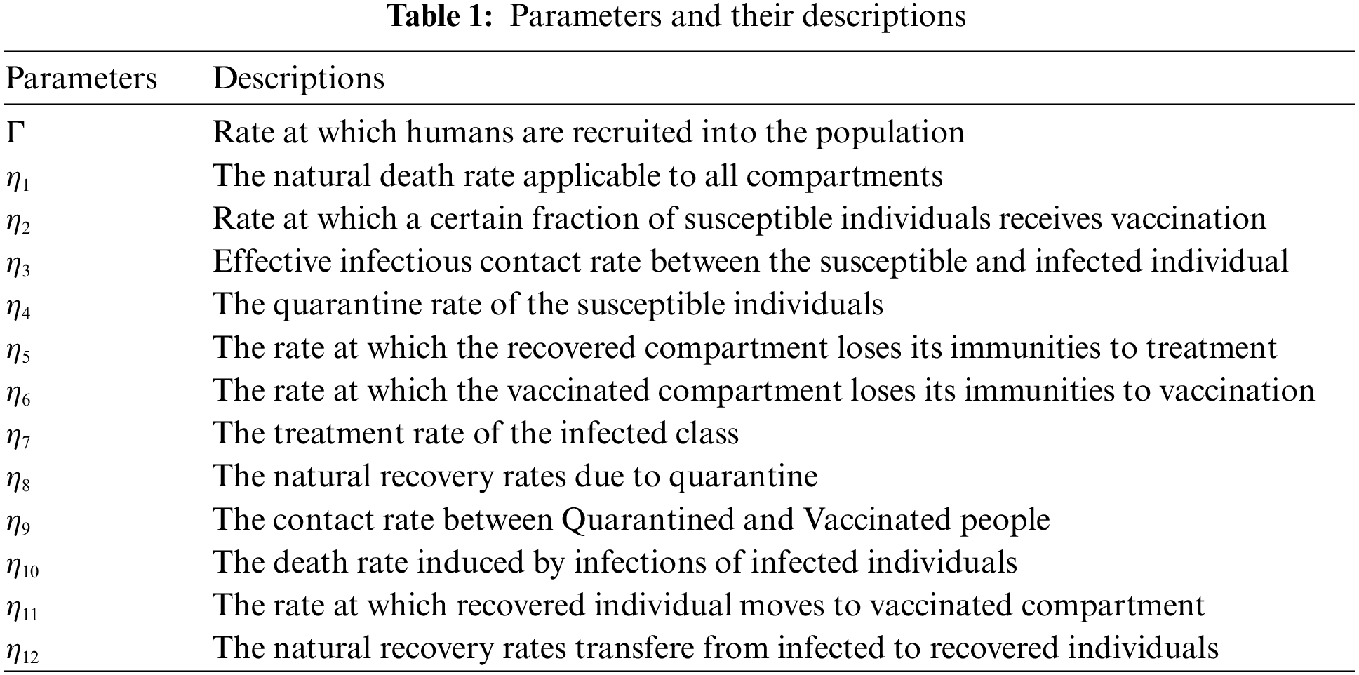
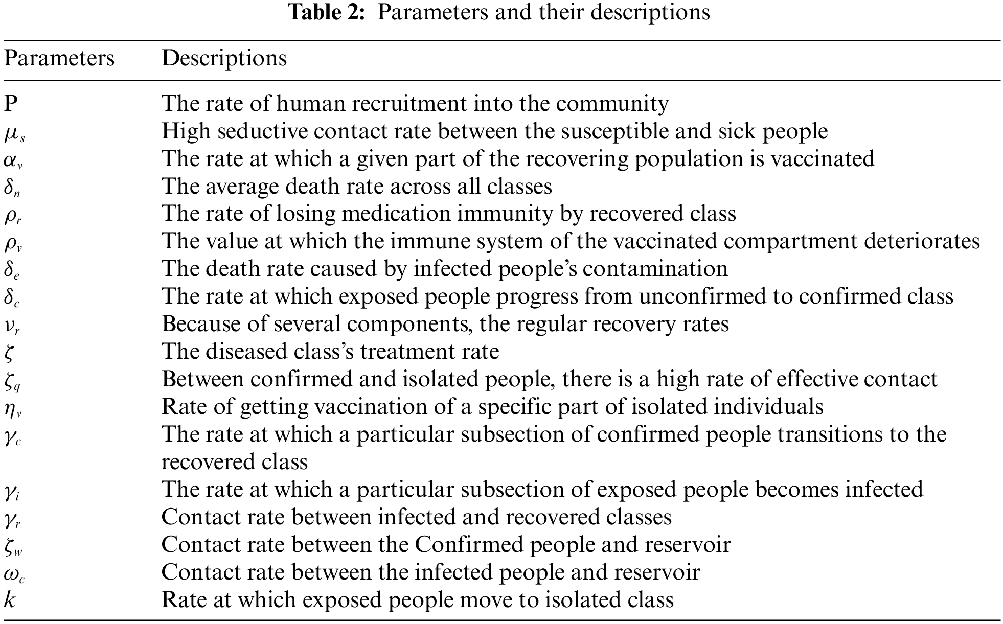
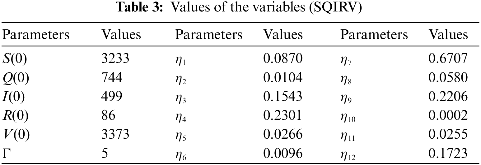
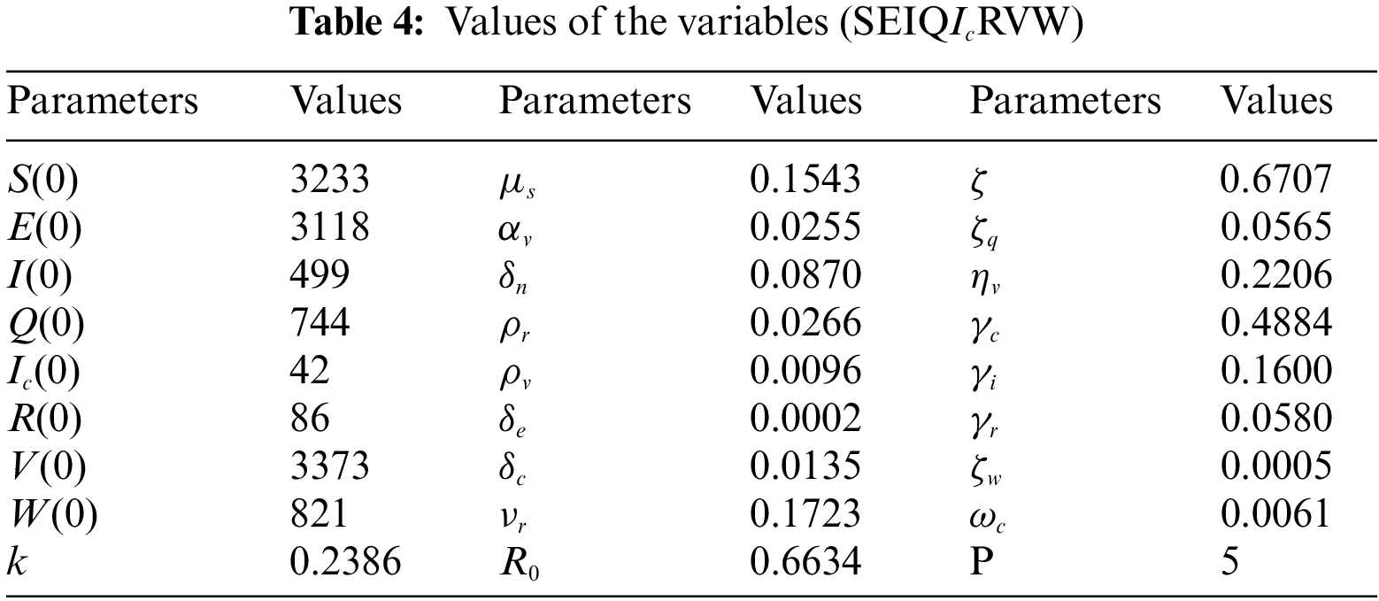
During the second wave of the Corona virus, India experienced a high infection rate. We obtained data for this article from Tamilnadu, India. This current Omicron variant pandemic data of Tamilnadu, India is validated with our theoretical findings. The source of the data is specified by [28] and [23]. Tamil Nadu encountered its most memorable instance of the Omicron type of SARS-CoV-2 on December 15, 2021, as indicated by a traveller from another country. Three weeks after the first confirmed Omicron case was reported, Tamil Nadu was infected with the highly transmissible and rapidly spreading form of SARS-Cov-2. The data for this study is gathered from the state of Tamil Nadu (Chennai). As of March 11, 2022, there were 750606 positive cases, 750520 discharged cases, 48 deaths, 499 active cases, 42 positive cases on March 11, 2022, 86 recovered cases, and 3373 vaccinated cases. The state of Tamilnadu achieves a zero-death rate and a safe position against the spread of Omicron on March 11, 2022. We used Mathematica for plotting the solution. The values of the variables and parameters are listed in the Tables 3 and 4 below.
The susceptible individual curves for the systems SEIQ
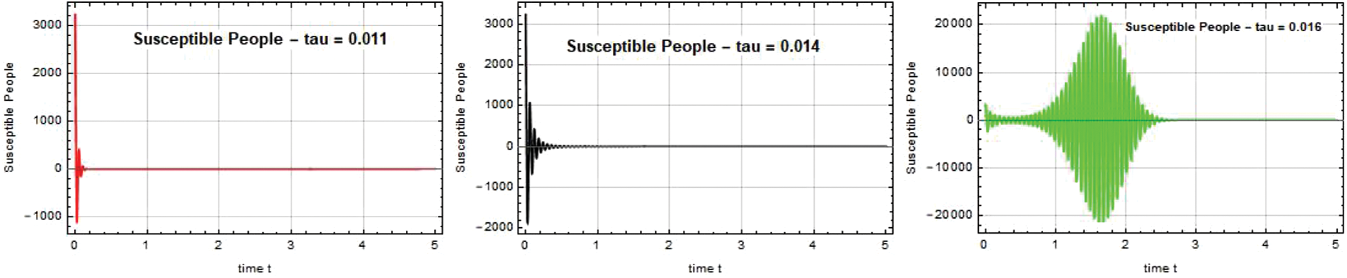
Figure 1: Susceptible people S(t) against time t with various
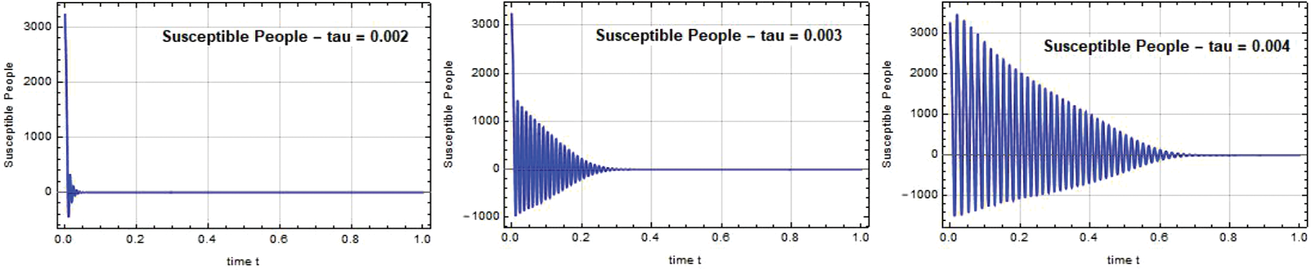
Figure 2: Susceptible people S(t) against time t with various
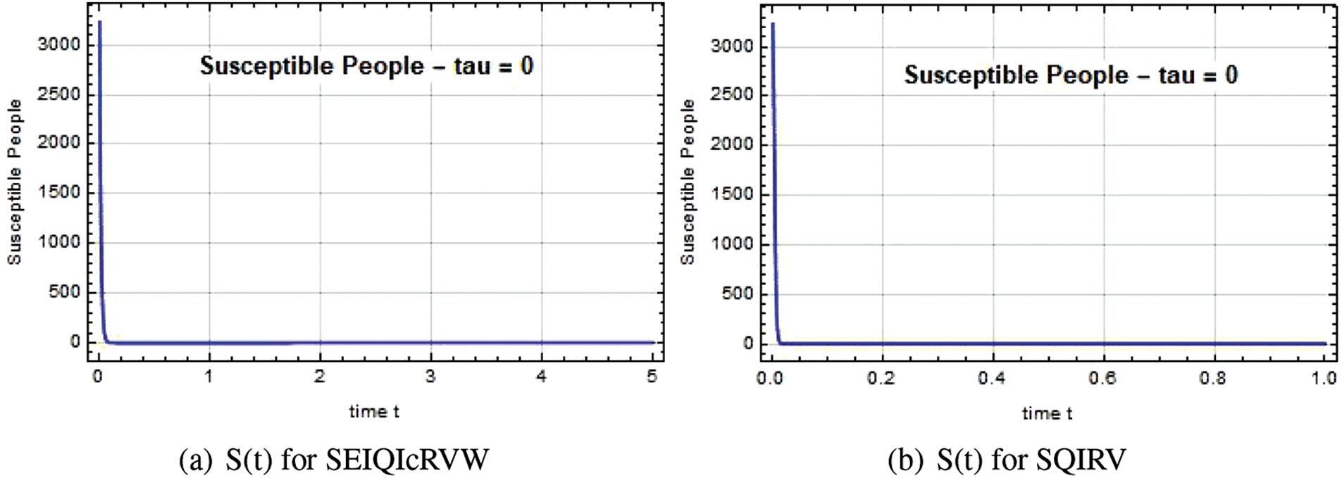
Figure 3: Susceptible people S(t) against time t with
Fig. 4 demonstrates that when the exposed population decreases, the population of other compartments also decreases, while when the exposed population rises, the population of all related compartments rises.
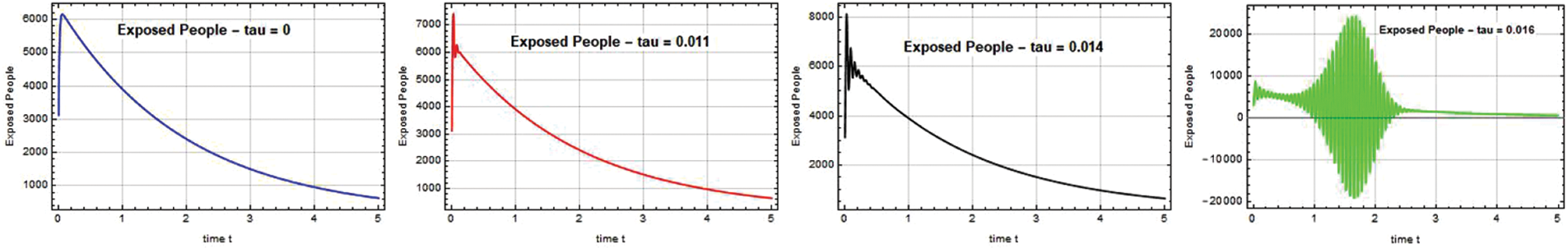
Figure 4: Exposed people E(t) against time t with various
Figs. 5–7 illustrate the possible reduction in the Omicron infection rate. Fig. 5 demonstrates that when the Omicron variant was first discovered, its spread was rapid, and that the variant’s spread was reduced to a safe level when the government implemented quarantine and vaccination at a high rate. By adding more compartments from the models that came before it, the SEIQ
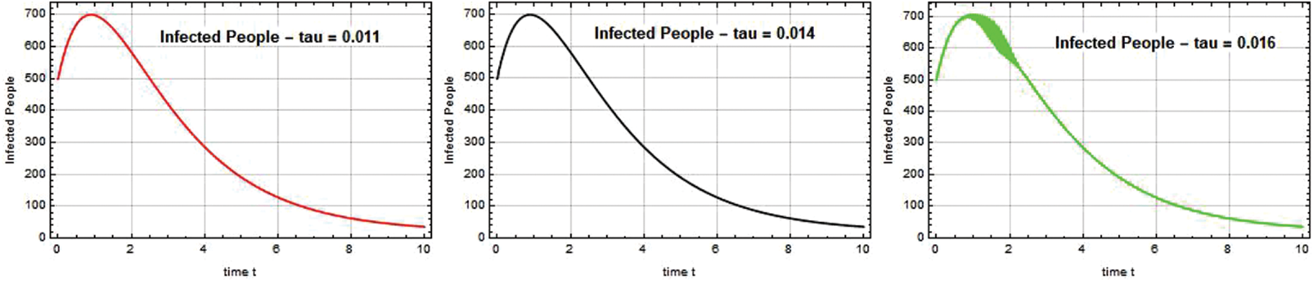
Figure 5: Infected people I(t) against time t with various
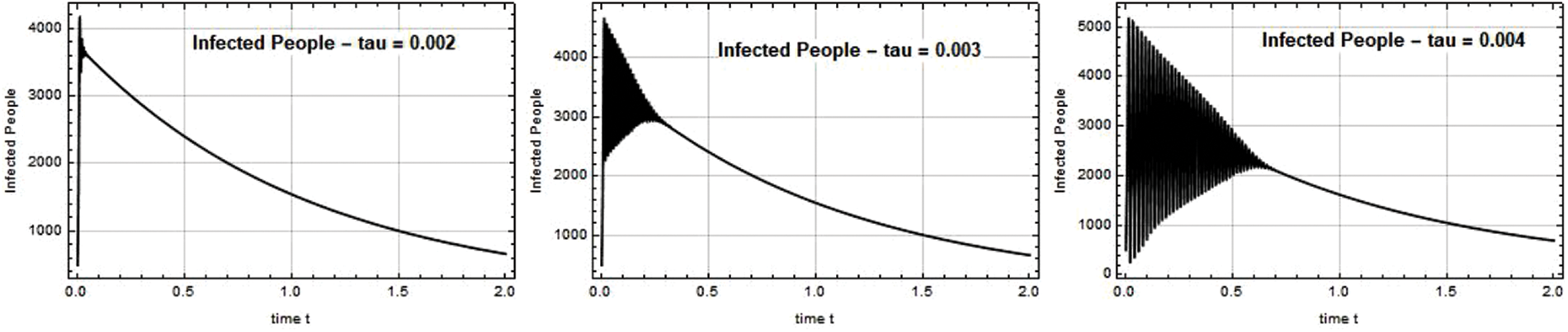
Figure 6: Infected people I(t) against time t with various
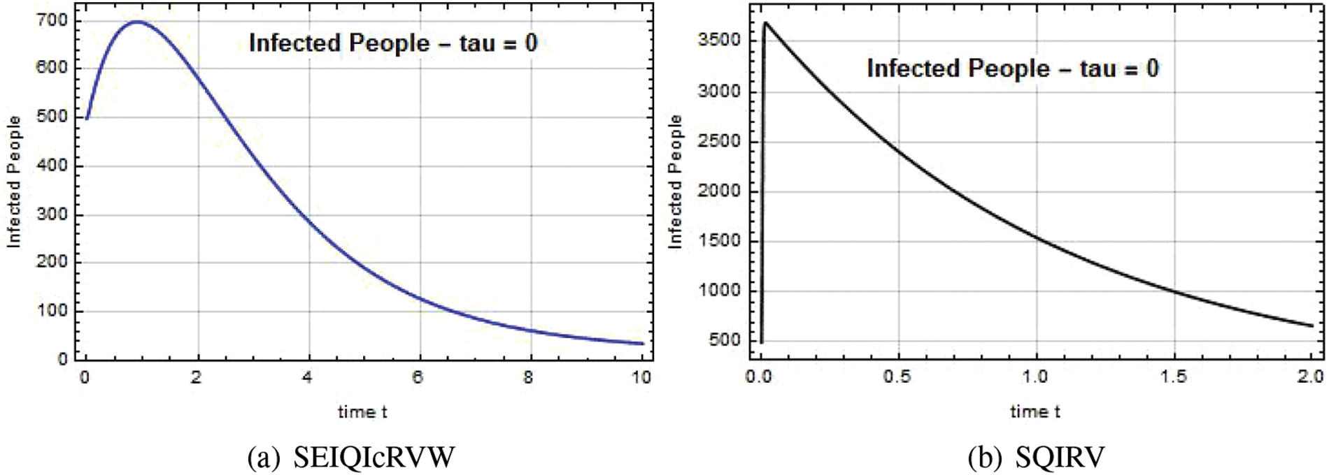
Figure 7: Infected people I(t) against time t with
The Quarantined individual level at time t is depicted in Figs. 8–10. When the government implemented the quarantine in Chennai at a high range, the spread of the disease was contained, and the situation in Chennai returned to normal.

Figure 8: Quarantined people Q(t) against time t with various
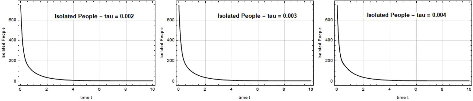
Figure 9: Quarantined people Q(t) against time t with various
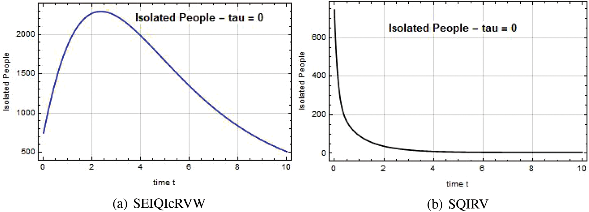
Figure 10: Quarantined people Q(t) against time t with
According to Fig. 11, the population of these four districts experiences a high rate of illness during the Omicron period, which begins on December 25 and ends on March 11, 2022. The infection rate gradually decreased to a low level and there were no deaths when people were vaccinated in accordance with government instructions.
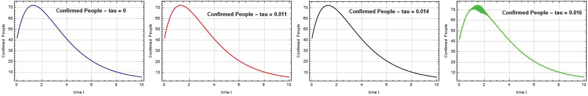
Figure 11: Confirmed people S(t) against time t with various
Reproduction numbers of 0.66, 0.92, 0.63, and 0.06 for SEIQ
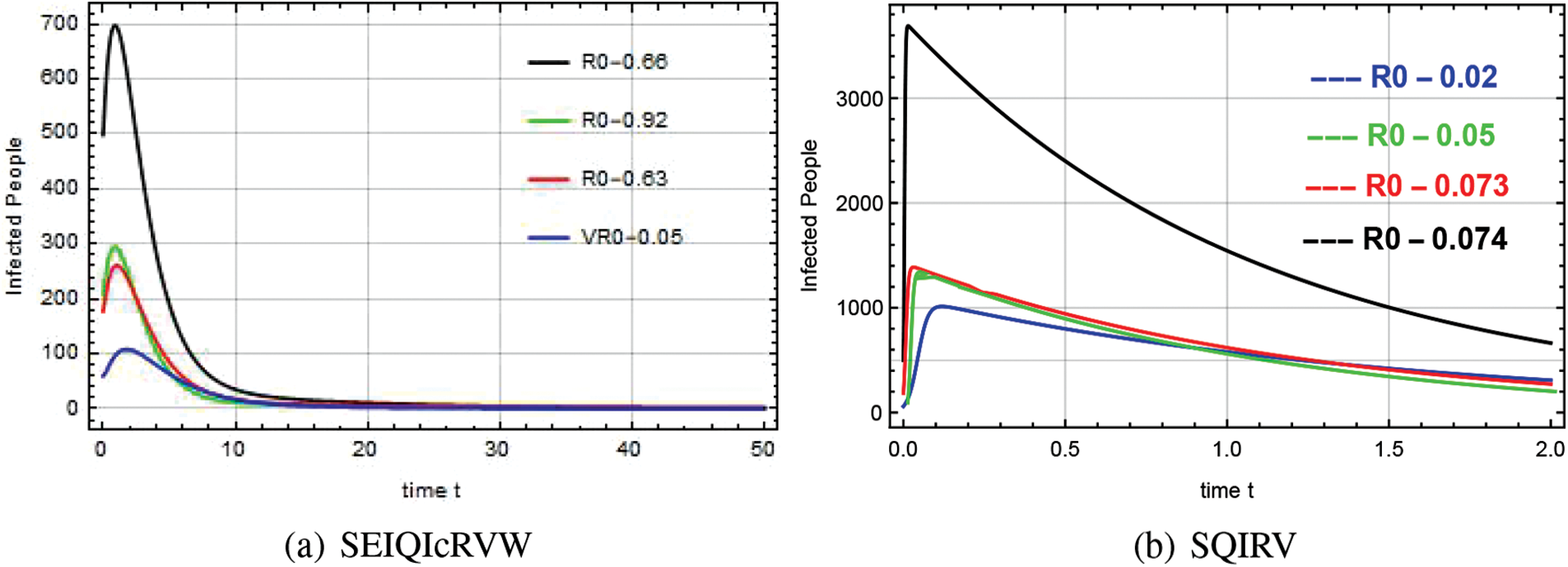
Figure 12: Infected range about various reproduction numbers for the system SEIQ
The rise in recovered rates for both systems in Chennai is depicted in Figs. 13–15. By balancing the recovered and infected rates with standard rates, the system SEIQ

Figure 13: Recovered people R(t) against time t with various
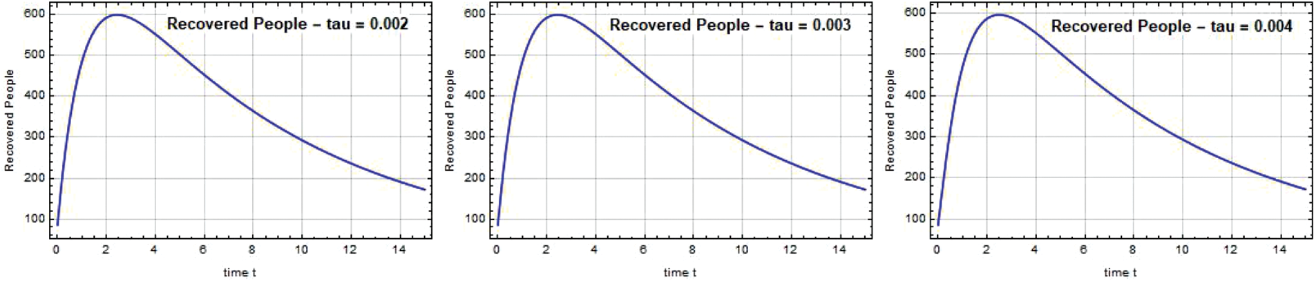
Figure 14: Recovered people R(t) against time t with various

Figure 15: Recovered people R(t) against time t with
The rapid rise in the number of people being vaccinated is depicted in Figs. 16–18. As a result, the system’s infection rate significantly decreased, and the system became stable. The significance of vaccination to the Omicron virus control strategy is demonstrated by these figures.
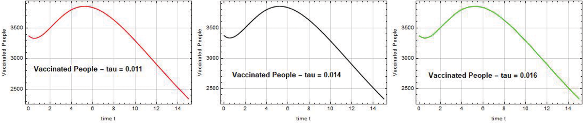
Figure 16: Vaccinated people V(t) against time t with various

Figure 17: Vaccinated people V(t) against time t with various

Figure 18: Vaccinated people V(t) against time t with
The effect of delayed SEIQ

Figure 19: Reservoir people W(t) against time t with various

Figure 20: Stability of the system SEIQI

Figure 21: Stability of the system SQIRV against time t with various
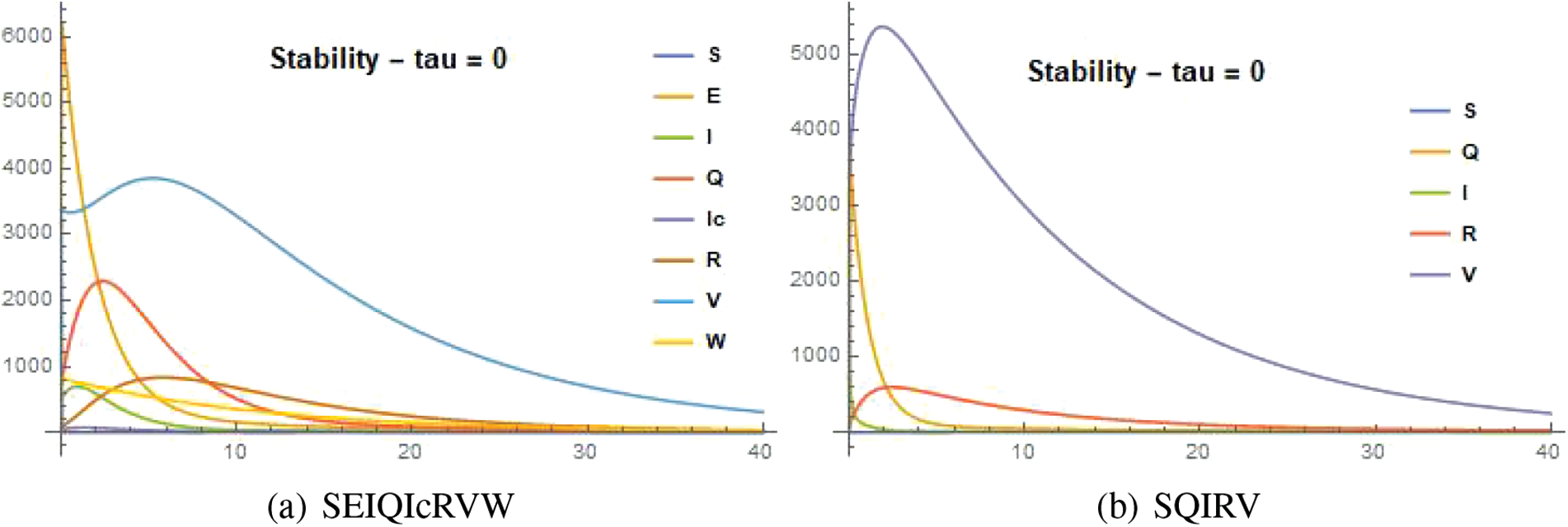
Figure 22: Stability of the systems with
Novel delayed mathematical models for the Omicron B.1.1.529 SARS-Cov-2 Variant were developed in this paper. The stability of the two models has been examined and validated, and the principles of reproduction number calculated with this model are an outbreak threshold that determined whether or not the disease would spread further in the district Chennai of Tamilnadu. As the figures show, infection-free steady-state solutions are locally asymptotically stable when
Acknowledgement: This study is supported via funding from Prince Sattam bin Abdulaziz University Project Number (PSAU/2023/R/1444). The first author is partially supported by the University Research Fellowship (PU/AD-3/URF/21F37237/2021 dated 09.11.2021) of Periyar University, Salem. The second author is supported by the fund for improvement of Science and Technology Infrastructure (FIST) of DST (SR/FST/MSI-115/2016).
Funding Statement: This study is supported via funding from Prince Sattam bin Abdulaziz University Project Number (PSAU/2023/R/1444). The first author is partially supported by the University Research Fellowship (PU/AD-3/URF/21F37237/2021 dated 09.11.2021) of PeriyarUniversity, Salem. The second author is supported by the fund for improvement of Science and Technology Infrastructure (FIST) of DST (SR/FST/MSI-115/2016).
Author Contributions: S. Dickson: Conceptualization, Visualization, Software, Resources, Formal analysis, Investigation, Writing-original draft. S. Padmasekaran: Investigation, Supervision, Formal analysis, Writing-review & editing. P. Kumar: Investigation, Supervision, Formal analysis, Writing-review & editing. Kottakkaran Sooppy Nisar: Investigation, Supervision, Formal analysis, Writing-review & editing. Hamidreza Marasi: Investigation, Supervision, Formal analysis, Writing-review & editing.
Availability of Data and Materials: Data sharing not applicable to this article as no datasets were generated or analyzed during the current study.
Conflicts of Interest: The authors declare that they have no conflicts of interest to report regarding the present study.
References
1. Byul Nim, K., Eunjung, K., Sunmi, L., Chunyoung, O. (2020). Mathematical model of COVID-19 transmission dynamics in South Korea: The impacts of travel, social distancing and early detectio. Processes, 8(10), 1304. [Google Scholar]
2. Chatzarakis, G. E., Dickson, S., Padmasekaran, S. (2022). A dynamic SIqIRV mathematical model with non-linear force of isolation, infection and cure. Nonautonomous Dynamical System, 9(1), 56–67. [Google Scholar]
3. Daniel Deborah, O. (2020). Mathematical model for the transmission of COVID-19 with nonlinear forces of infection and the need for prevention measure in nigeria. Journal of Infectious Diseases and Epidemiology, 6(5), 1–12. [Google Scholar]
4. Kiran, R., Madhumita, R., Syed, A., Taraphder, A. (2021). Effect of population migration and punctuated lockdown on the spread of infectious diseases. Nonautonomous Dynamical System, 8(1), 251–266. [Google Scholar]
5. Maski Tomochi, M. K. (2021). A mathematical model for COVID-19 pandemic-SIIR model: Effects of asymptomatic individuals. Journal of General and Family Medicine, 22(1), 5–14. [Google Scholar] [PubMed]
6. Sudhanshu Kumar, B., Jayanta Kumar, G., Susmita, S., Uttam, G. (2020). COVID-19 pandemic in India: A mathematcal model study. Nonlinear Dynamics, 102(1), 1–17. [Google Scholar]
7. Swati, T., Shaifu, G., Syed, A., Krishna, P., Baazaoui, R. (2021). Analysis of infectious disease transmission and prediction through SEIQR epidemic model. Nonautonomous Dynamical Systems, 8(1), 75–86. [Google Scholar]
8. Ashwin, M., Balamuralitharan, S., Poongodi, M., Mounir, H., Kaamran, R. et al. (2022). Stability and numerical solutions of second wave mathematical modeling on COVID-19 and omicron outbreak strategy of pandemic: Analytical and error analysis of approximate series solutions by using HPM. Mathematics, 10(3), 343. [Google Scholar]
9. Wang, B. G., Wang, Z. C., Wu, Y., Xiong, Y. P., Zhang, J. P. et al. (2022). A mathematical model reveals the in the influence of NPIs and vaccination on SARS-CoV-2 omicron variant. Nonlinear Dynamics, 111(4), 3937–3952. [Google Scholar] [PubMed]
10. Dickson, S., Padmasekaran, S., Kumar, P. (2023). Fractional order mathematical model for B.1.1.529 SARS-CoV-2 omicron variant with quarantine and vaccination. International Journal of Dynamics and Control, 11(5), 2215–2231. [Google Scholar]
11. Kumar, P., Suat Erturk, V. (2021). A case study of COVID-19 epidemic in India via new generalised caputo type fractional derivatives. Mathematical Methods in Applied Sciences, 2021, 1–14. [Google Scholar]
12. Kurkina E. S., Koltsova E. M. (2021). Mathematical modeling of the propagation of COVID-19 pandemic waves in the world. Computational Mathematics and Modeling, 32(2), 147–170. [Google Scholar]
13. Pakwan, R., Sherif, E., Arthi, I. (2021). A mathematical model of COVID-19 pandemic: A case study of bangkok, Thailand. Computational and Mathematical Methods in Medicine, 6664483, 1–11. [Google Scholar]
14. Kumar, P., Govindaraj, V., Zareen, A. K. (2022). Some novel mathematical results on the existence and uniqueness of generalized Caputo-type initial value problems with delay. AIMS Mathematics, 7(6), 10483–10494. [Google Scholar]
15. Liu, Z., Magal, P., Seydi, O., Webb, G. (2020). A COVID-19 epidemic model with latency period. Infectious Disease Modelling, 5, 323–337. [Google Scholar] [PubMed]
16. Yang, C., Yang, Y. L., Li, Z. W., Zhang, L. S. (2021). Modeling and analysis of COVID-19 based on a time delay dynamic model. AIMS Mathematical Biosciences and Engineering, 18(1), 154–165. [Google Scholar]
17. Sedighe, R., Noushin, A., Azadeh, S. (2020). Application of distribution-delay models to estimating the hospitalized mortality rate of COVID-19 according to delay effect of hospitalizations counts. Journal of Biostatatistics and Epidemiology, 6(4), 241–250. [Google Scholar]
18. Yang, F. F., Zhang, Z. Z. (2021). A time-delay COVID-19 propagation model considering supply chain transmission and hierarchical quarantine rate. Advances in Difference Equations, 2021, 191. [Google Scholar] [PubMed]
19. Hameed, K. E., Nizar, A., Hussein, B., Ebraheem, S. (2021). Delayed dynamics of SIR model for COVID-19. Open Journal of Modelling and Simulation, 9(2), 146–158. [Google Scholar]
20. Shidong, Z., Guoqiang, L., Tao, H., Xin, W., Junli, T. et al. (2021). Vaccination control of an epidemic model with time delay and its application to COVID-19. Nonlinear Dynamics, 106, 1279–1292. [Google Scholar]
21. Giovanni, N., Carla, P., Salvatore, T., Giorgia, V. (2022). A time-delayed deterministic model for the spread of COVID-19 with calibration on a real dataset. Mathematics, 10(4), 661. [Google Scholar]
22. Mohamed Zaitri, A., Christiana, J., Delfim, F. (2022). Stability analysis of delayed COVID-19 models. Axioms, 11(8), 400. [Google Scholar]
23. Dickson, S., Padmasekaran, S., Chatzarakis, G. E., Panetsos, L. (2022). SQIRV model for Omicron variant with time delay. Australian Journal of Analysis and Applications, 19(2), 1–16. [Google Scholar]
24. Diekmann, O., Heesterbeek, J., Metz, J. (1990). On the definition and computation of the basic reproduction number R0 in models for infectious disease. Journal of Mathematical Biology, 28, 365–382. [Google Scholar] [PubMed]
25. Van den Driessche, P., Watmough, J. (2002). Reproduction number and sub threshold epidemic equilibrium for compartmental models for disease transmission. Mathematical Biosciences, 180(1–2), 29–48. [Google Scholar] [PubMed]
26. Niculescu, S. I. (2001). Delay effects on stability: Lecture notes in control and information sciences, vol. 269. London, UK: Springer. [Google Scholar]
27. Dickson, S., Padmasekaran, S., Chatzarakis, G. E. (2022). Stability analysis of B.1.1.529 SARS-cov-2 omicron variant mathematical model: The impacts of quarantine and vaccination. Nonautonomous Dynamical System, 9(1), 290–306. [Google Scholar]
28. IndiaFightsCorona COVID-19 (2022). https://www.mygov.in/covid-19 (accessed on 11/03/2022). [Google Scholar]
Cite This Article
 Copyright © 2024 The Author(s). Published by Tech Science Press.
This work is licensed under a Creative Commons Attribution 4.0 International License , which permits unrestricted use, distribution, and reproduction in any medium, provided the original work is properly cited.
 Downloads
 Citation Tools