Distributed Dynamic Load in Structural Dynamics by the Impulse-Based Force Estimation Algorithm

1  Introduction

Accurately reconstructing the dynamic forces acting on a structure holds significant importance in various engineering applications. Frequently, direct measurements of the input are not feasible, while limitations in practicality and cost prevent measurements of the structure’s response at all physical locations. In such cases, the forces must be indirectly determined from dynamic response measurements using system inversion techniques.

A distributed dynamic load, such as the air pressure load experienced by a building or the water pressure load on ships, plays a critical role in the analysis of dynamic loads. Therefore, the recognition of distributed dynamic loads has considerable practical significance. While numerous methods and techniques [1,2] were developed to identify concentrated dynamic loads, there remains a dearth of research focused on distributed dynamic loads, particularly in the area of time-domain recognition methods.

Two primary avenues have emerged for studying distributed dynamic loads: one involves the technology of spatial fitting, while the other emphasizes establishing load relationships in either the time or frequency domain. It is comparatively straightforward to identify the load with the frequency response function [3–6] in the frequency domain because the time series information is essentially lost in the frequency domain, thereby simplifying the calculation. The study of establishing a temporal relationship in load is primarily observed in the context of concentrated loads, as evident in the current scientific literature [1]. Several studies have employed a variety of methods to estimate concentrated or distributed dynamic loads, primarily using Green’s kernel function to discretize the acceleration response. For example, Li et al. [7,8] and Wan et al. [9] used the direct inverse method of discretized Green’s kernel function to establish the relationship between load and response in the time domain. Kazemi et al. [10] applied the trapezoidal rule to improve the accuracy of the discretization method of Green’s kernel function. Liu et al. [11] proposed a time domain Galerkin method based on discretized Green’s kernel function. The studies on the aforementioned time-domain techniques can be grouped together, encompassing two main steps. The first step involves mathematically formulating the mapping from input sequences to output sequences using an operational matrix, resulting in a large matrix. The second step focuses on solving the ill-posed inverse problem through the application of a regularization method. Many papers have studied ill-conditioned inverse problems. For example, Wang et al. [12,13] adopted a new homotopy perturbation method and a new iterative regularization method, Wang et al. [14] employed Tikhonov regularization, while Liu [15] utilized the multi-vector iterative algorithm in a Krylov subspace. However, when the dimension of the matrix is significantly increased, it becomes challenging or even impossible to solve the matrix and identify the force. Liu et al. [16] and Jiang et al. [17] attempted to establish the load-response relationship in the time domain using the Newmark method. Furthermore, a recursive approach for load identification through joint input-state estimation was developed by Meas et al. [18] and Lourens et al. [19]. Li et al. [20] innovatively calculated the relationship of concentrated loads in the time domain using function principles. As described above, these methods [16–20] are used in the identification of concentrated loads. In the space fitting technique, shape functions [21,22], basic functions [16], and generalized orthogonal polynomials [3–6] have been widely employed. In addition, Wu et al. [23–25] have conducted research on the identification of randomly distributed dynamic loads. However, these studies do not involve fixed-frequency excitation, particularly low-frequency excitation associated with significant structural damage. In addition to parametric methods, there are non-parametric methods such as artificial intelligence. Artificial intelligence [16,26,27] can recognize the structure of the training target through a large number of prior trainings. However, this black box method is challenging to explain at the principal level, so its applicability needs to be enhanced for structural dynamics, which are sensitive to shape and boundary conditions.

This paper presents the Impulse-based Force Estimation Algorithm (IFEA), in which the recursive algorithm based on convolution integral combined with the moving mean and polynomial fitting methods can avoid the inversion of super-high dimensional matrices and, as a result, can accurately identify loads with a long history and fast-changing characteristics over time. For distributed dynamic load, the utilization of polynomial function and modal analysis has proven successful in converting a dynamic load, which encompasses two dimensions of space and time, into coefficient identification for a single-degree-of-freedom (SDOF) system. Ultimately, the successful identification of distributed dynamic loads with a sufficiently long duration and diverse forms on a continuum with an infinite number of degrees of freedom is achieved in the time domain, in contrast to the frequency domain proposed in [3–6], rather than the concentrated loads proposed in [16–20]. Moreover, the method employs acceleration response instead of strain proposed in [21,28], making it more convenient to measure in engineering applications.

The theoretical framework of this study commences with Section 2, which details the process of dimension reduction for the distributed dynamic load and provides a mathematical derivation of the IFEA. In Section 3, the proposed method is validated with numerical simulations, followed by experimental verification of the IFEA in Section 4. Section 5 presents the conclusion of this research.

2  Principle of Distributed Dynamic Load Identification

A conventional point-load excitation is inherently constrained in terms of spatial degrees of freedom, with a mathematical form of f(x1,x2,⋅⋅⋅,xn,t), where x1,x2,⋅⋅⋅,xn are discrete variables. However, distributed dynamic loads, characterized by the mathematical form f(x,t), exhibit infinite-dimensional spatial degrees of freedom. Consequently, the identification and calculation of distributed dynamic loads present substantial challenges. Additionally, a limited number of measurement points in engineering applications further complicates the estimation of infinite-dimensional distribution loads based on such limited data.

2.1 Dimension Reduction

For deterministic structures, modal parameters can be obtained with modal testing or finite-element modal-analysis technique [29]. The introduction of modal coordinates simplifies the problem of identification, reducing it to that of a typical SDOF system. Let us consider the bending vibration of a Bernoulli-Euler simply supported beam in a continuous system. By introducing the modal coordinates w(x,t)=ϕn(x)qn(t), the vibration equation for this scenario is represented by Eq. (1).

q¨n(t)+2ωnζnq˙n(t)+ωn2qn(t)=fn(t)mn.(1)

where n stands for modal order. qn(t), q˙n(t) and q¨n(t) denote modal displacement, model velocity and modal acceleration of each order, respectively. ωn and ζn represent natural frequency and damping ratio of each order. mn is a modal mass and fn(t) is a modal force of each order after mass normalization, given by fn(t)=∫0lϕn(x)f(x,t)dx. l is the beam length. The modal truncation frequency is typically set at 1.5 times the maximum dynamic response frequency, with a maximum limit of not exceeding 2 times. Modes beyond this frequency range have negligible contributions to the dynamic response, aligning with the principle of the modal superposition method for calculating dynamic response.

For decoupled SDOF systems, the distributed dynamic load f(x,t) can be transformed into fn(t). When time is discretized, the fitting target in this case is fn(tj), where tj is the discrete and known time. If the objective of the fitting is fn(tj), it becomes possible to achieve dimensionality reduction from two dimensions to one because fn(tj) is a scalar quantity, also referred to as the modal force for each discrete time. Even if an analytical solution for the integral of x cannot be obtained, there exists an approximate numerical solution at tj. Through modal analysis, the distributed dynamic load is effectively reduced from the two dimensions of t and x to the numerical values of each mode at discrete time instants, thereby achieving dimensionality reduction of the unknown variables. In this manner, time and space can be simultaneously identified in the form of modal force, without the need for sequential recognition of time and spatial functions.

2.2 Recursion Principle of IFEA

Eq. (1) can be calculated using the convolution integral expressed in Eq. (2),

q(t)=∫0th(t−τ)f(τ)dτ.(2)

Here, h(t−τ)=e−ζω(t−τ)sin⁡(ωd(t−τ))mωd and ωd=ω1−ζ2. It should be noted that the modal order, represented by n, is not explicitly indicated in Eq. (2).

Considering a SDOF damped system subjected to an excitationf(t), in a separate sampling interval [tjtj+1], the responses of the two endpoints tj and tj+1 are known, enabling the determination of the two unknowns of the functional form of the force within the sampling interval [tjtj+1]. Assuming that the function of the force in the sampling interval [tjtj+1] is denoted as Eq. (3),

f(t)=a0+a1t.(3)

Theoretically, Eq. (3) can be uniquely determined based on the aforementioned two response points. Moreover, if the sampling interval is sufficiently small, it can be assumed that the excitation force undergoes an approximately linear change within the interval [tjtj+1]. This establishes a relationship between the force described by a first-order polynomial and the arbitrary excitation function, as depicted in Fig. 1. Once the force within the interval [tjtj+1] is expressed by Eq. (3), its response at a specific time t within the interval can be expressed as the sum of the three responses shown in Eq. (4), based on the principle of linear superposition,

x(t)=x1(t)+x2(t)+x3(t).(4)

Figure 1: Schematic illustration of recursion principle

Among these, x1(t) is the displacement of free vibration resulting from the displacement x(tj) and velocity x˙(tj) at time tj. x2(t) represents the displacement response caused by a rectangular pulse with an amplitude of a0. Similarly, x3(t) represents the displacement response caused by a triangular pulse with a slope of a1.

Upon substituting Eq. (3) into Eq. (2), the results are

x2(t)=a0∫0th(t−τ)dτ,(5)

x3(t)=a1∫0th(t−τ)τdτ.(6)

From the perspective of impulse, Eqs. (5) and (6) are equivalent to Eqs. (7) and (8),

x2(t)=f(tj)∫0th(t−τ)dτ,(7)

x3(t)=f(tj+1)−f(tj)tj+1−tj∫0th(t−τ)τdτ.(8)

Within each discrete time interval, the integrand function of the convolution integral comprises known quantities, including the constant basis, basis t, and unit impulse response function. Hence, the convolution integral can provide an analytical solution. There is an inherent analytical solution for x1(t), so arranging x1(t), x2(t), and x3(t) yields,

{x1(t)=e−ζωt[x(tj)cos⁡ωdt+x˙(tj)+ζωx(tj)ωdsin⁡ωdt]x2(t)=f(tj)k[1−e−ζωt(cos⁡ωdt+ζωωdsin⁡ωdt)]x3(t)=f(tj+1)−f(tj)(tj+1−tj)kω2[ω2t−2ζω+e−ζωt(2ζωcos⁡ωdt−ωd2−ζ2ω2ωdsin⁡ωdt)].(9)

where k is the stiffness. By taking the first and second derivatives of t, the acceleration and velocity can be obtained as Eq. (10),

{x˙(t)=x˙1(t)+x˙2(t)+x˙3(t)x¨(t)=x¨1(t)+x¨2(t)+x¨3(t).(10)

The calculated velocity is shown in Eq. (11),

{x˙1(t)=e−ζωt[−(x(tj)ωd+ζωx˙(tj)+ζωx(tj)ωd)sin⁡ωdt+x˙(tj)cos⁡ωdt]x˙2(t)=f(tj)ω2kωde−ζωtsin⁡ωdtx˙3(t)=f(tj+1)−f(tj)(tj+1−tj)k[1−e−ζωt(cos⁡ωdt+ζωωdsin⁡ωdt)].(11)

The calculated acceleration is given by Eq. (12),

{x¨1(t)=e−ζωt[(ω2ζωx(tj)+x˙(tj)ωd−2x˙(tj)ωd)sin⁡ωdt−(2ζωx˙(tj)+ω2x(tj))cos⁡ωdt]x¨2(t)=f(tj)ω2ke−ζωt(cos⁡ωdt−ζωωdsin⁡ωdt)x¨3(t)=[f(tj+1)−f(tj)]ω2e−ζωtsin⁡ωdt(tj+1−tj)kωd.(12)

At the end of the time interval tj+1, t becomes equal to tj+1−tj. Thus, in Eqs. (9), (11) and (12), there are only four unknowns, namely, the displacement x(tj) at time tj, the velocity x˙(tj) at time tj, the force f(tj) at time tj and the force f(tj+1) at time tj+1. Define Δt=tj+1−tj, and combine the same terms for the above four unknowns in Eqs. (4) and (10) to obtain Eq. (13),

{x(tj+1)=C1x(tj)+C2x˙(tj)+(C1−C4)f(tj)+C4f(tj+1)x˙(tj+1)=C5x(tj)+C6x˙(tj)+(C7−C8)f(tj)+C8f(tj+1)x¨(tj+1)=C9x(tj)+C10x˙(tj)+(C11−C12)f(tj)+C12f(tj+1).(13)

Here, C1 to C12 are defined as follows:

C1=e−ζωΔt(cos⁡ωdΔt+ζωωdsin⁡ωdΔt), C2=1ωde−ζωΔtsin⁡ωdΔt,

C3=1k(1−C1), C4=1Δtk(Δt−2ζωmC3−C2), C5=−ω2C2,

C6=C1−2ζωC2, C7=1mC2, C8=1ΔtC3, C9=−ω2C1+2ω2ζωC2, C10=(4ζ2ω2−ω2)C2−2ζωC1, C11=1m(C1−2ζωC2) and C12=1ΔtmC2.

The convolution integration takes the form of a parametric integral in mathematics, namely the form F(x)=∫c(x)d(x)f(x,y)dy. The derivative rule is shown in Eq. (14),

F ′(x)=f(x,d(x))d ′(x)−f(x,c(x))c ′(x)+∫c(x)d(x)∂f(x,y)∂xdy.(14)

Eqs. (15) and (16) can be obtained by Eq. (14),

{x˙(t)=∫0th˙(t−τ)f(τ)dτh˙(t−τ)=∂h(t−τ)∂t=e−ζω(t−τ)m[cos⁡ωd(t−τ)−ζωωdsin⁡ωd(t−τ)],(15)

{x¨(t)=f(t)+∫0th¨(t−τ)f(τ)dτh¨(t−τ)=e−ζω(t−τ)[(ζ2ω2−ωd2)sin⁡ωd(t−τ)−2ζωωdcos⁡ωd(t−τ)]mωd.(16)

Eqs. (15) and (16) represent velocity and the acceleration in the form of convolution integral. It can be seen from Eqs. (2), (15), and (16) that at time 0, acceleration experiences a sudden change due to excitation, consistent with Newton’s second law. However, displacement and velocity do not experience such sudden changes due to excitation. Therefore, the recognition of initial excitation can be obtained from Eq. (16). Consequently, a recursive relationship in time is established for all discrete time of the excitation force. Fig. 2 displays the flowchart for force estimation.

Figure 2: Flow chart of recursion

The method reconstructs information regarding the force within the interval and a recursion relationship was established for the load between the two discrete points. This approach enables efficient handling of a large number of sampling points, as each step only requires solving the equation at the current moment. Specifically, for 10,000 sampling points, a matrix with 10,000 rows and 10,000 columns needs to be constructed according to references [7–10]. This matrix construction method is commonly referred to as the Green kernel function discretization method, which essentially discretizes acceleration. However, the method proposed in this paper only requires processing Eq. (13) for 10,000 times. For a larger number of sampling points, it is not feasible to calculate a super large-scale non-sparse matrix using conventional methods and equipment. Moreover, these matrices are often ill-conditioned in load identification, necessitating the use of regularization methods to process the matrix. The recursion based on convolution integral, however, does not suffer from such disadvantages, greatly increasing the engineering significance of our method. Of course, multiple iterations can introduce trend errors, which are described in the following section.

2.3 Trend Elimination of IFEA

Through experiments and simulations, we have observed that multiple iterations can lead to cumulative errors. To visualize these errors, we introduced the concept of Direct Current (DC) in the circuit, which we refer to as DC trends. According to the process shown in Fig. 2, the error of force estimation affects the entire process. After conducting numerous simulations and experiments, we have found that for a SDOF system, although the recognition result after multiple iterations exhibits a DC trend, the relative load estimation remains accurate. This means that the identified load fluctuates around the DC trend with the correct relative amplitude.

To address the issue of DC trend, we incorporate a moving mean filtering algorithm. Let us consider a set of time-series discrete signals denoted as s(i), where i represents the number of sampling points and belongs to the range of non-negative integers. We define the moving window size as k. When k is an odd number, the window is centered on the current element. When k is even, the window includes the current element and its previous element, resulting in an odd-sized window. If there are insufficient elements to fill the window at the end, the window will be automatically truncated. In such cases, the average is calculated only based on the elements within the window. Mathematically, the moving mean is represented as Eq. (17),

s¯=1k[s(i)+s(i+1)+⋅⋅⋅+s(i+k−1)].(17)

The schematic diagram is depicted in Fig. 3.

Figure 3: Schematic diagram of the moving mean

In the absence of a DC trend, the moving mean remains relatively constant. However, when a DC trend is present, the moving mean also changes, reflecting the trend value. The sliding window should be appropriately sized according to the sampling rate and frequency of the response. As the moving mean is calculated using a sliding window, any change in the input signal’s characteristics will cause fluctuations at the junctions of the two segments. To address this issue, we employ a polynomial fitting method to fit the DC trend of each segment. By using a polynomial, we perform fitting based on the least square index to approximate the DC trend from the sampled signal. Once the DC trend is fitted, it can be removed from the recognized excitation signal.

2.4 Spatial Dimension Reconstruction

Section 2.1 converts the continuous system into a SDOF system with multiple modes, while Section 2.2 establishes a recursive form in a SDOF system. Now it is merely necessary to establish the relationship between the SDOF systems and the actual response, and each order of modal force can be solved based on the actual response. At a specific discrete time tj, the modal forces of each order are denoted as fn(tj). Assuming there are k measuring points, the following system of linear equations can be constructed according to the modal analysis theory:

x¨(x1,tj)=∑n=1∞ϕn(x1)[Cn9x(tj−1)+Cn10x˙(tj−1)+(Cn11−Cn12)fn(tj−1)+Cn12fn(tj)]x¨(x2,tj)=∑n=1∞ϕn(x2)[Cn9x(tj−1)+Cn10x˙(tj−1)+(Cn11−Cn12)fn(tj−1)+Cn12fn(tj)]⋮x¨(xk,tj)=∑n=1∞ϕn(xk)[Cn9x(tj−1)+Cn10x˙(tj−1)+(Cn11−Cn12)fn(tj−1)+Cn12fn(tj)].(18)

where n still stands for modal order. Typically, the number of measuring points will be greater than the modal truncation order. Therefore, Eq. (18) can be rapidly solved using the least square solution, and the modal forces of each order at the discrete time fn(tj) can be obtained.

In accordance with Section 2.1, the modal force at discrete time tj is given by,

fn(tj)=∫0lϕn(x)f(x,tj)dx.(19)

This study assumes that the spatial distribution function of the distributed dynamic load displays spatial smoothness, indicating a low spatial frequency. Consequently, multi-order polynomials are utilized to approximate it. The modal load of each order at discrete time tj can be obtained as Eq. (20),

fn(tj)=∫0lϕn(x)[dxxdxx2dx⋯xkdx][a0a1a2⋯ak]T.(20)

where a0 to ak represent polynomial coefficients for each order. For multiple modes, Eq. (20) expands to,

[f1(tj)f2(tj)⋮fn(tj)]=[∫0lϕ1(x)dx∫0lϕ1(x)xdx⋯∫0lϕ1(x)xkdx∫0lϕ2(x)dx∫0lϕ2(x)xdx⋯∫0lϕ2(x)xkdx⋮⋮⋮∫0lϕn(x)dx∫0lϕn(x)xdx⋯∫0lϕn(x)xkdx][a0a1⋮ak].(21)

where n stands for modal order, as in the previous case. Eq. (21) can be abbreviated as,

F=HA.(22)

The matrix H is a small-scale matrix whose size depends solely on the modal order and the polynomial order. As a result, the coefficient matrix A can be obtained by,

A=H+F.(23)

Hence, the distributed dynamic load at discrete time tj can be obtained, and subsequently, the distributed dynamic load at each discrete time can be determined based on modal forces at corresponding discrete time. When calculating the spatial distribution of the distributed dynamic load, each discrete time is independent of one another, and there is no mutual influence of errors. This overcomes the vulnerability of multi-order polynomials to error sensitivity.

3  Results of Simulation Validation and Discussion

3.1 Evaluation Index

In order to objectively and quantitatively describe the obtained dynamic load, commonly used signal evaluation methods should be adopted. Let the theoretical load signal at time j be X(j), and the reconstructed signal at time j be Y(j). The following equation defines the normalized mean error of square (NMES),

NMES=∑j=0n[X(j)−Y(j)]2∑j=0nX(j)2×100%.(24)

where n is the number of discrete points. The smaller the value of this index, the closer the identification is to the theoretical value. The correlation coefficient method (CCM) is also introduced as an evaluation criterion, as demonstrated by Eq. (25),

CCM=∑i=1n[X(i)−X¯][Y(i)−Y¯]∑i=1n[X(i)−X¯]2∑i=1n[Y(i)−Y¯]2×100%.(25)

Here, X¯ and Y¯ respectively represent the mean value of X(i) and Y(i), n also represents the number of discrete points, and the correlation coefficient is employed to signify the degree of correlation between the theoretical signal X(i) and the recognized signal Y(i), with a maximum value of 100% that indicates complete consistency between the two pieces of information. The closer the value is to 100%, the stronger the correlation between the two signals, indicating higher recognition accuracy.

3.2 Fixed Frequency Plus Random Excitation

The IFEA is validated for the SDOF system depicted in Fig. 4. The system parameter is set to m=5kg, k=200 N/m and c=0.1N⋅s/m. the form of the applied load is sin⁡(3πt)+10sin⁡(5πt). Additionally, a noise with a mean of 0 and a standard deviation of 1 is superimposed on the excitation to simulate random excitation. Since random excitation should be represented in the form of a power spectrum, simulating rapidly changing random excitation using noise is convenient in this context.

Figure 4: Schematic diagram of the SDOF system

The acceleration response of the example is illustrated in Fig. 5, the identified dynamic load is depicted in Fig. 6, and the rating index is presented in Fig. 7.

Figure 5: Response of acceleration

Figure 6: Estimation of force

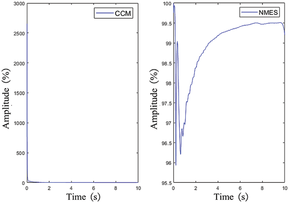
Figure 7: The index of the example

Fixed frequency plus random excitation is a common condition in engineering, and the time-domain algorithm has the potential to identify the excitation after fixed frequency and random superposition simultaneously. However, this requires a smaller sampling interval and more sampling points. It can be observed from Fig. 6 that the estimated force is largely consistent with the applied excitation. The error indicator drops rapidly and approaches zero, except for the initial point where the applied stimulus is zero, leading to a significant amplification of the error. The correlation coefficient steadily increases during the identification process, indicating a growing similarity between the two signals. The example demonstrates that IFEA can accurately identify dynamic loads in the time domain, including long time-history loads, which is unachievable with the discrete Green’s function.

3.3 Distributed Dynamic Load of Fixed Frequency

In the field of structural dynamics, low-frequency loads induce low-order modes in a structure, which typically exhibit larger amplitudes and have the potential to cause more damage. On the other hand, high-frequency loads are often treated as random loads acting upon the structure in engineering scenarios. Consequently, a simply supported beam model with a remarkably low first-order mode was specifically designed, as depicted in Fig. 8. The beam has a length of 2 m and a rectangular cross-sectional shape with dimensions of 0.02 m×0.003 m (width × height). The material properties of the beam are characterized by an elastic modulus of 70 GPa, a density of 2700 kg/m3, and a damping of 0.1 N⋅s/m. The first five natural frequencies of the simply supported beam are determined as 1.7, 6.9, 15.6, 27.7, and 43.3 Hz, respectively.

Figure 8: Simply-supported beam and boundary conditions

The distributed dynamic load, acting perpendicular to the beam, is described by the equation sin⁡(180 t)cos⁡(0.5 πx)/2+0.7. This load exhibits an excitation frequency of approximately 28.6 Hz, effectively stimulating the fourth-order mode. The sampling step is defined as 0.0005 s, resulting in a sampling rate of 2000 Hz. A total duration of 1s is considered, resulting in a total of 2001 sampling points. The chosen measurement positions were 0.5, 0.9, 1.1, 1.3 and 1.7 m, as shown in Fig. 8, which theoretically facilitate the determination of the fourth-order polynomial. The measuring point does have an effect on the result of identification. Selecting the location of the sampling points is a complex matter. The most crucial aspect is that the measurement point information should encompass as much modal information as possible, and the dynamic response of the measurement point should be uncorrelated. This is also the principle of selecting measuring points in this paper. The selection of measuring points has significant criteria, which can be specifically viewed in papers [30,31] on optimal sensor placement. The selection of the number of measurement points is dependent on the order of modal truncation. In the case of the four modes, at least four measuring points are required to uniquely determine each mode force.

The form of the load is shown in Fig. 9.

Figure 9: Original load: (a) three-dimensional view; (b) x-z view; (c) x-y view

The estimation of each order of modal force is depicted in Fig. 10, while the index of modal force is illustrated in Fig. 11. Furthermore, the three-dimensional distributed dynamic load identified is presented in Fig. 12.

Figure 10: Modal forces: (a) first order (b) second order (c) third order (d) fourth order

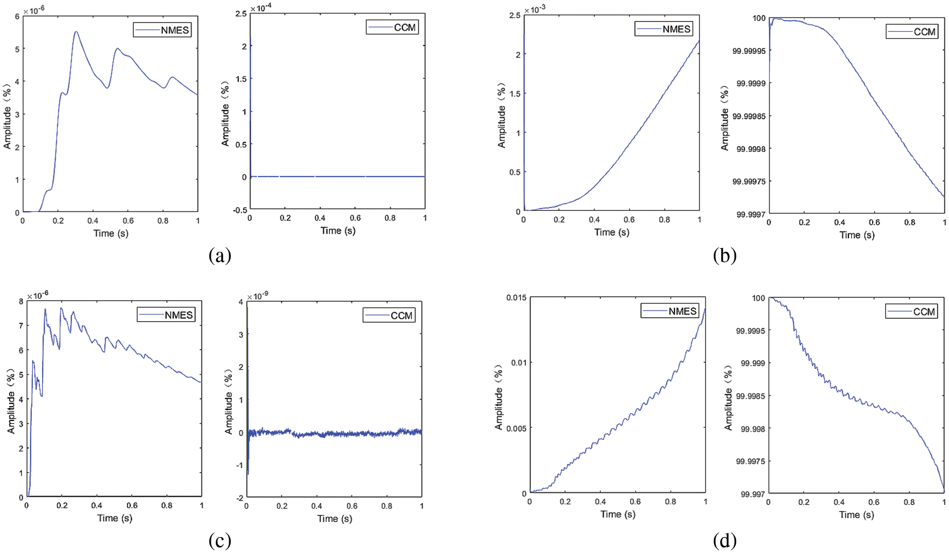
Figure 11: NMES and CCM: (a) first order (b) second order (c) third order (d) fourth order

Figure 12: Reconstructed load: (a) three-dimensional view; (b) x-z view; (c) x-y view

Due to the linear nature of the first-order and third-order modal forces, the correlation coefficient index yields a poor result and loses its functionality. However, by observing the NMES index and the modal force curve, it is evident that the identified force fluctuates around a straight line with minimal error. Overall, both the modal force curves and the index curves indicate a highly accurate recognition of each order of modal force.

The errors between the reconstructed and original loads are shown in Fig. 13.

Figure 13: Errors of reconstructed load: (a) three-dimensional view; (b) x-z view

As depicted in Fig. 13, the absolute error is extremely small and nearly zero in the middle. The increase in error at both ends can be attributed to the inherent error in fitting trigonometric functions with polynomials. The utilization of spatial distribution in the form of trigonometric functions aims to demonstrate that any error in the spatial fitting of each step remains confined to the space of the current step and does not impact the accuracy of the modal force in the time domain. Consequently, spatial errors do not result in cumulative errors over time. This observation is further supported by Fig. 13, as the spatial error does not exhibit an increase with an escalation in the number of recurrence steps.

3.4 Distributed Dynamic Load Undergone a Mutation

Furthermore, to validate the method’s estimation capability for rapidly changing and long time-history loads, we devised an excitation that undergoes a mutation. The mutation of this excitation alternates in both spatial distribution and frequency, thereby testing the method’s recognition ability. The form of excitation is shown in Eq. (26),

f(x,t)={12cos⁡(180t)cos⁡(π2x),0≤t<0.512[cos⁡(180t)sin⁡(π2x)−cos⁡(90)sin⁡(π2x)+cos⁡(90)cos⁡(π2x)],0.5≤t<212[sin⁡(182t)sin⁡(π2x)−sin⁡(364)sin⁡(π2x)+cos⁡(360)sin⁡(π2x)−cos⁡(90)sin⁡(π2x)+cos⁡(90)cos⁡(π2x)],2≤t.(26)

The excitation is continuous in the time domain. All other conditions remain unchanged from the previous example, with the only alteration being the extension of sampling time to three seconds. The form of excitation is illustrated in Fig. 14.

Figure 14: Original load: (a) three-dimensional view; (b) x-z view; (c) x-y view

As evident from Fig. 14, there is a successive mutation in both the spatial distribution and frequency. The estimation of each order of modal force is depicted in Fig. 15, while the modal force index is illustrated in Fig. 16. Furthermore, the three-dimensional distributed dynamic load identified is presented in Fig. 17.

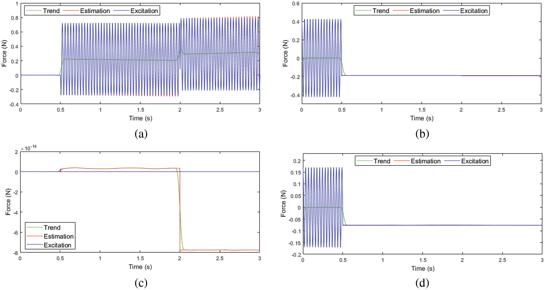
Figure 15: Modal forces: (a) first order (b) second order (c) third order (d) fourth order

Figure 16: NMES and CCM: (a) first order; (b) second order; (c) third order

Figure 17: Reconstructed load: (a) three-dimensional view; (b) x-z; (c) x-y view

The third-order modal force is represented by a straight line with a value of 0, and it is evident from the figure that the identification is highly accurate. Hence, calculating its index is not possible as the denominator of the index becomes extremely small, resulting in an infinite value. Similarly, this applies to the first 0.5 s of the first-order modal force, so the index for the first-order modal force is calculated starting from 0.5 s. The modal force diagram and all indices demonstrate the accuracy of the estimated force.

The errors between the reconstructed and original loads are shown in Fig. 18.

Figure 18: Errors of reconstructed load: (a) three-dimensional view; (b) x-z view

The example demonstrates that the proposed method can effectively identify long time-history distributed dynamic loads undergone a mutation, with highly accurate identification results and minimal error.

3.5 Robustness to Noise

To assess the method’s robustness against noise, we introduced 2% Gaussian white noise to the response stimulated in Section 3.3 for noise simulation, while keeping everything else unchanged. The modal force is depicted in Fig. 19, the index is illustrated in Fig. 20, and the fitted distributed dynamic load error is showcased in Fig. 21.

Figure 19: Modal forces with noise: (a) first order (b) second order (c) third order (d) fourth order

Figure 20: NMES and CCM: (a) first order (b) second order (c) third order (d) fourth order

Figure 21: Reconstructed error for load with noise: (a) three-dimensional view; (b) x-z view

The first and third order modal force indices can also be elucidated by the analysis in Section 3.3. From the aforementioned figures, it is evident that the method possesses a certain level of noise resistance. Nevertheless, since the assessment of dynamic load relies on the accuracy of acceleration response, any inaccuracies in the acceleration response will inevitably impact the precision of load estimation.

4  Results of Experimental Verification and Discussion of Algorithm

The modal force for single-point concentrated loads is given by Eq. (27),

fn(t)=∫0lϕn(x)f(x,t)δ(x−x1)dx,(27)

where x1 signifies the position at which the load is applied.

About contributions of single-point concentrated to the response, it can be obtained similarly from Eq. (27) that the sole difference between concentrated loads and distributed lies in the modal force of each mode order, while all other factors remain constant.

Given the proposed nature of IFEA as a time-domain method in this study, it is feasible to employ experimental data comprising concentrated excitations to verify the algorithm’s performance in the time domain. Since concentrated dynamic loads are employed, the multi-order polynomial fitting is unnecessary during the computation process. Merely utilizing zero-order polynomial fitting is adequate. Among the various forms of concentrated excitations, impulsive loads, characterized by high amplitude and rapid variations, pose more stringent demands on numerical computations, particularly in terms of load tracking in the time domain and accuracy of amplitude reconstruction [32,33].

Considering the challenges associated with controlling and measuring spatially distributed dynamic loads, including difficulties in accurately controlling the amplitude of distributed loads in the spatial domain and challenges in measuring the amplitude of continuously distributed dynamic loads. These challenges can lead to significant errors in experimental data, thereby impeding the validation of the algorithm itself. Therefore, the validation procedure uses the mature and easily controllable concentrated dynamic load to emphasize the performance of the time domain of the newly proposed IFEA. If the experiment incorporates impulse loads, it would provide an opportunity to evaluate the performance of the IFEA under an impulse load. Additionally, this would serve as a supplementary demonstration of simulations. Thus, a pulsive load is the excitation source during the experimental validation process.

The configuration of the simply supported beam model is depicted in Fig. 22, while the structural and material parameters can be found in Table 1.

Figure 22: Physical model

A modal experiment was performed on the simply supported beam employing the hammer impact technique, wherein the natural frequencies and modal damping ratios of the simply supported beam were measured and are presented in Table 2.

Given the instantaneous characteristics and brief duration of impact loads, there are stringent demands for dynamic-load identification algorithms. To assess the accuracy of amplitude recognition, the peak relative error is introduced,

PRE=|maxY(i)−maxX(i)|maxX(i)×100%.(28)

An impact load was imparted using a force hammer at a distance of 0.37 m. Accelerometers were strategically positioned at response point 1 (located at 0.28 m) and response point 2 (located at 0.49 m) to capture the acceleration responses, as depicted in Fig. 23.

Figure 23: Experimental diagram

Notably, in the magnified section of Fig. 24, the dynamic response promptly initiates after 0.49 s, signifying the application of the impact load on the beam is between 0.49 and 0.492 s.

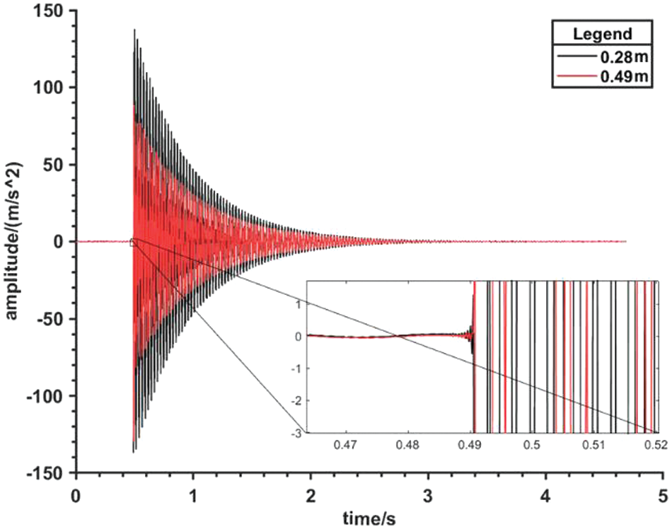
Figure 24: Acceleration response to impact load

The reconstructed load is shown in Fig. 25.

Figure 25: Reconstructed impact load

Similarly, in the identified impact-load graph, the zoomed-in segment illustrates the load attaining its peak at 0.492 s and commencing its effects between 0.49 and 0.492 s. These findings affirm the experiment’s success in verifying the algorithm’s precision in reconstructing the load duration. In Fig. 24, the temporal and amplitude values of the peaks are visually discernible, with the peak relative error calculated using Eq. (28) amounting to 17.96%. Overall, this algorithm accurately determines the application time of the impact load and reasonably determines its amplitude and trend. Although this paper focuses on distributed dynamic loads, it can be observed from experiments and Eq. (27) that when the concentrated loads and distributed loads are converted into modal forces at a specific discrete time, there is no significant difference in their forms, and both are scalar. Therefore, the algorithm can still accurately identify the modal forces. This is why the experiment is conducted to verify the algorithm with a concentrated load that is easily controlled and accurately measured. Hence, this method can also identify a specific form of distributed dynamic load, namely a point load, on the premise of knowing the position of the point load. For an unknown position of the point load or a moving point load, the method cannot determine the excitation position, so it needs to be adjusted accordingly.

5  Conclusion

In this study, a novel approach for distributed load identification in the time domain is introduced. The novelty of the methodology can be summarized as follows:

(1) By employing polynomials and modal analysis, the task of recognizing a dynamic distribution load which has two dimensions of space and time is converted into the identification of coefficients within a single-degree-of-freedom system. This method can effectively reduce the dimension of the system and recognize the spatial and temporal distribution simultaneously in the form of model force. In coefficient recognition, each step of the reconstruction is solely based on the modal force at the current time. This prevents the accumulation of spatial reconstruction errors and has no impact on the errors in the time domain. Through this approach, the distributed dynamic loads on a continuum are effectively established, not for discrete systems with multiple degrees of freedom, nor for concentrated loads.

(2) Based on the convolution integral, a recursive algorithm is proposed. The recursive scheme possesses the ability to calculate long time-history loads undergone a mutation in the time domain. This is an ability that ultra-high-dimensional matrices, which require regularization, do not possess. Utilizing the response of the sampling point, the algorithm reconstructs the force in the sampling interval while considering the pulse energy. This enhancement obtains the analytical solution of the convolution integral of the reconstructed force in discrete time, instead of assuming a constant interval force. Additionally, the method employs acceleration response instead of strain, making it easier to measure in engineering applications.

(3) The strategy of moving mean and polynomial fitting to eliminate trend is introduced, providing IFEA with the capability to accurately estimate the dynamic loads of structures in the time domain.

As demonstrated by the examples, IFEA possesses the capability to estimate rapidly changing loads in the time domain after converting the loads into modal space, which is also an advantage of this algorithm. However, when identifying the spatial distribution, this paper assumes a smooth spatial distribution of load. For loads that exhibit significant spatial variations, higher-order polynomials are necessary for fitting, but correspondingly more measurement points are required, potentially leading to overfitting. However, as the spatial distribution recognition is confined to each individual step, any inaccuracy in spatial recognition does not impact the accuracy of the modal forces in the time domain.

Acknowledgement: The invaluable advice of Tian Tang during the preparation of this experiment is greatly appreciated. We are also grateful to the editors and reviewers for their helpful suggestions.

Funding Statement: The authors received no specific funding for this study.

Author Contributions: The authors confirm contribution to the paper as follows: study conception and design: Yuantian Qin, Yucheng Zhang; data collection: Yucheng Zhang; analysis and interpretation of results: Yuantian Qin, Yucheng Zhang; draft manuscript preparation: Yucheng Zhang, Vadim Silberschmidtb. All authors reviewed the results and approved the final version of the manuscript.

Availability of Data and Materials: The data used in this paper has been made available within the paper. Moreover, the data supporting the findings can be obtained from the corresponding author upon a reasonable request.

Conflicts of Interest: The authors declare that they have no conflicts of interest to report regarding the present study.

References

1. Liu, R. X., Dobriban, E., Hou, Z. C., Qian, K. (2022). Dynamic load identification for mechanical systems: A review. Archives of Computational Methods in Engineering, 29(2), 831–863. [Google Scholar]

2. Wang, L., Liu, Y. R., Xu, H. Y. (2021). Review: Recent developments in dynamic load identification for aerospace vehicles considering multi-source uncertainties. Transactions of Nanjing University of Aeronautics and Astronautics, 38(2), 271–287. [Google Scholar]

3. Jiang, J. H., Kong, H. F., Yang, H. J., Chen, J. D. (2021). One identification method of distributed dynamic load based on modal coordinate transformation for thin plate structure. International Journal of Computational Methods, 18(7), 2150012. https://doi.org/10.1142/S0219876221500122 [Google Scholar] [CrossRef]

4. Jiang, J. H., Luo, S. Y., Zhang, F. (2021). One novel dynamical calibration method to identify two-dimensional distributed load. Journal of Sound and Vibration, 515, 116465. https://doi.org/10.1016/j.jsv.2021.116465 [Google Scholar] [CrossRef]

5. Qin, Y. T., Chen, G. P., Zhang, F. (2012). Moment method of two-dimensional distributed dynamic load identification. Journal of Vibration, Measurement & Diagnosis, 32(1), 34–41 (In Chinese). [Google Scholar]

6. Qin, Y. T. (2012). Two-dimensional wavelet-Galerkin method for distributed load identification. Journal of Vibration, Measurement & Diagnosis, 32(6), 1005–1009 (In Chinese). [Google Scholar]

7. Li, K., Liu, J., Han, X., Sun, X. S., Jiang, C. (2015). A novel approach for distributed dynamic load reconstruction by space-time domain decoupling. Journal of Sound and Vibration, 348, 137–148. [Google Scholar]

8. Li, K., Liu, J., Han, X., Jiang, C., Zhang, D. Q. (2017). Distributed dynamic load identification based on shape function method and polynomial selection technique. Inverse Problems in Science and Engineering, 25(9), 1323–1342. [Google Scholar]

9. Wan, C., Yan, B. (2017). A time domain identification method for distributed dynamic loads on 1D spatial structures. Applied Mathematics and Mechanics, 38(9), 967–978 (In Chinese). [Google Scholar]

10. Kazemi, A. A., Bucher, C. (2015). Derivation of a new parametric impulse response matrix utilized for nodal wind load identification by response measurement. Journal of Sound and Vibration, 344, 101–113. [Google Scholar]

11. Liu, J., Meng, X. H., Jiang, C., Han, X., Zhang, D. Q. (2016). Time-domain Galerkin method for dynamic load identification. International Journal for Numerical Methods in Engineering, 105(8), 620–640. [Google Scholar]

12. Wang, L. J., Xu, H., Xie, Y. X. (2011). A new homotopy perturbation method for solving an ill-Posed problem of multi-source dynamic loads reconstruction. Computer Modeling in Engineering & Sciences, 82(3–4), 179–194. [Google Scholar]

13. Wang, L. J., Han, X., Xie, Y. X. (2012). A new iterative regularization method for solving the dynamic load identification problem. Computers, Materials & Continua, 31(2), 113–126. [Google Scholar]

14. Wang, L., Liu, J. K., Lu, Z. R. (2020). Bandlimited force identification based on Sinc-dictionaries and Tikhonov regularization. Journal of Sound and Vibration, 464, 114988. https://doi.org/10.1016/j.jsv.2019.114988 [Google Scholar] [CrossRef]

15. Liu, C. S. (2013). An optimal multi-vector iterative algorithm in a Krylov subspace for solving the ill-posed linear inverse problems. Computers, Materials & Continua, 33(2), 175–198. [Google Scholar]

16. Liu, Y. R., Wang, L., Li, M., Wu, Z. M. (2022). A distributed dynamic load identification method based on the hierarchical-clustering-oriented radial basis function framework using acceleration signals under convex-fuzzy hybrid uncertainties. Mechanical Systems and Signal Processing, 172, 108935. https://doi.org/10.1016/j.ymssp.2022.108935 [Google Scholar] [CrossRef]

17. Jiang, J. H., Ding, M., Li, J. (2021). A novel time-domain dynamic load identification numerical algorithm for continuous systems. Mechanical Systems and Signal Processing, 160, 107881. https://doi.org/10.1016/j.ymssp.2021.107881 [Google Scholar] [CrossRef]

18. Meas, K., Smyth, A. W., De, R. G., Lombaert, G. (2016). Joint input-state estimation in structural dynamics. Mechanical Systems and Signal Processing, 70–71, 445–466. [Google Scholar]

19. Lourens, E., Reynders, E., De, R. G., Degrande, G., Lombaert, G. (2012). An augmented Kalman filter for force identification in structural dynamics. Mechanical Systems and Signal Processing, 27, 446–460. [Google Scholar]

20. Li, H. Q., Jiang, J. H., Cui, W. X., Zhao, J. M., Mohamed, M. S. (2022). One novel dynamic-load time-domain-identification method based on function principle. Applied Sciences, 12(19), 9623. https://doi.org/10.3390/app12199623 [Google Scholar] [CrossRef]

21. Zheng, Y., Wu, S. Q., Fei, Q. G. (2021). Distributed dynamic load identification on irregular planar structures using subregion interpolation. Journal of Aircraft, 58(2), 288–299. [Google Scholar]

22. Li, X. W., Zhao, H. T., Chen, Z., Chen, J. A. (2020). Identification of distributed dynamic excitation based on Taylor polynomial iteration and cubic Catmull-Rom spline interpolation. Inverse Problems in Science and Engineering, 28(2), 220–237. [Google Scholar]

23. Wu, S. Q., Yin, J., He, Z. H., He, D. D., Chen, S. H. (2022). Experimental study on base acceleration excitation and interface load identification on a satellite structure. Journal of Astronautics, 43(3), 319–327 (In Chinese). [Google Scholar]

24. Wu, S. Q., Sun, Y. W., Li, Y. B., Fei, Q. G. (2019). Stochastic dynamic load identification on an uncertain structure with correlated system parameters. Journal of Vibration and Acoustics, 141(4), 041013. https://doi.org/10.1115/1.4043412 [Google Scholar] [CrossRef]

25. Wu, S. Q., He, Z. H., Yin, J., Chen, S. H. (2022). Identification of annularly distributed random dynamic load between satellite and rocket in the frequency domain. Journal of Southeast University (Natural Science Edition), 52(5), 825–832 (In Chinese). [Google Scholar]

26. Zhou, J. M., Dong, L. L., Guan, W., Yan, J. (2019). Impact load identification of nonlinear structures using deep recurrent neural network. Mechanical Systems and Signal Processing, 133, 106292. https://doi.org/10.1016/j.ymssp.2019.106292 [Google Scholar] [CrossRef]

27. Qiu, B. B., Zhang, M., Li, X., Qu, X. Q., Tong, F. S. (2020). Unknown impact force localization and reconstruction in experimental plate structure using time-series analysis and pattern recognition. International Journal of Mechanical Sciences, 166, 105231. https://doi.org/10.1016/j.ijmecsci.2019.105231 [Google Scholar] [CrossRef]

28. Wang, Y. H., Zhou, Z. H., Xu, H., Li, S., Wu, Z. J. (2021). Inverse load identification in stiffened plate structure based on in situ strain measurement. Structural Durability & Health Monitoring, 15(2), 85–101. https://doi.org/10.32604/sdhm.2021.014256 [Google Scholar] [CrossRef]

29. Sarmast, M., Ghafari, H., Wright, J. (2019). Experimental and numerical study of structural identification using non-linear resonant decay method. Sound & Vibration, 53(3), 75–95. https://doi.org/10.32604/sv.2019.04193 [Google Scholar] [CrossRef]

30. Qin, X. R., Zhan, P. M., Yu, C. Q., Zhang, Q., Sun, Y. T. (2021). Health monitoring sensor placement optimization based on initial sensor layout using an improved partheno-genetic algorithm. Advances in Structural Engineering, 24(2), 252–265. [Google Scholar]

31. Qin, B. Y., Lin, X. K., Zhang, L. M., Guo, Q. T. (2011). Optimal sensor placement based on integer-coded genetic algorithm. Journal of Vibration and Shock, 30(2), 252–257 (In Chinese). [Google Scholar]

32. Kulkarni, R. B., Gopalakrishnan, S., Trikha, M. (2020). Impact force identification in structures using time domain spectral finite elements. Acta Mechanica, 231(11), 4513–4528. [Google Scholar]

33. Li, Q. F., Lu, Q. H. (2016). Impact localization and identification under a constrained optimization scheme. Journal of Sound and Vibration, 366, 133–148. [Google Scholar]