An Improved Bounded Conflict-Based Search for Multi-AGV Pathfinding in Automated Container Terminals

1  Introduction

Automated guided vehicles (AGVs) are the primary tool for container transport and crucial pieces of equipment for horizontal transportation operations in automated terminals. The number of AGVs is growing, which also causes issues like waiting, conflict, and deadlock in the operation of the equipment. These issues are caused by manual operation, large-scale operation, and the rising difficulty of intelligent terminals. At the level of automated terminals, increasing AGV operating speed is a critical issue that must be resolved since it has an impact on the efficiency of AGV transportation.

In various scenarios, research has been conducted on challenges related to multi-AGV path planning, spanning warehouses [1], electric vehicles [2], and terminals [3]. It closely addresses the challenges of job dispatch, scheduling, and routing. For warehouses and workshops, Yuan et al. [4] proposed a bi-level path planning algorithm employing an improved A* method at the first level and a rapidly exploring random tree approach at the second level to enhance search effectiveness. Wang et al. [5] suggested using a heuristic ant colony algorithm to solve the model, demonstrating its efficacy. Fazlollahtabar et al. [6] utilized a modified network simplex algorithm (NSA) to optimize the model. Ivica et al. [7] based their approach on a vehicle priority scheme to resolve conflicts. Chen et al. [8] utilized the ant agent optimized by a repulsive potential field to improve collision avoidance, transportation distance, and efficiency. Li et al. [9] proposed a novel quantum ant colony optimization algorithm that combines the advantages of various methods. Choi et al. [10] proposed a QMIX-based scheme for cooperative path control of multiple AGVs. For automated container terminals, Guo et al. [11] proposed an improved Dijkstra algorithm and an enhanced acceleration control method to solve the path planning problem for 42 AGVs. Hu et al. [12] combined the A* algorithm with a time window principle to plan each AGV’s path, with a maximum of 12 AGVs. Zhong et al. [13] validated the effectiveness of a hybrid genetic algorithm particle swarm optimization (HGA-PSO) in solving path planning problems for 24 AGVs. Zhong et al. [14] utilized a priority-based speed control strategy in conjunction with the Dijkstra depth-first search algorithm to solve the model. The AGV scheduling problem has been established as an non-deterministic polynomial (NP)-hard problem [15]. Luo et al. [16] proposed a genetic algorithm to obtain a mixed-integer linear optimization model (MILP), considering up to 10 AGVs. In existing literature, single-AGV path planning is often applied to solve multi-AGV path planning in automated container terminals (ACT). Simple traffic rules are employed when two AGVs might collide. However, as the number or density of robots increases, congestion occurs, leading to decreased system efficiency. In contrast, Multi-agent Path Finding (MAPF) plans paths for all AGVs simultaneously, considering various collision possibilities. Limited literature exists on multi-AGV path planning in ACT using the MAPF method.

MAPF problems involve finding the optimal set of paths from the starting position to the target position for multiple agents without conflicts. These problems can be divided into two classes: optimal and sub-optimal solvers. One approach to solving MAPF is by reducing it to other problems. For instance, Ma et al. [17] introduced a hierarchical algorithm within a Markov decision processes framework and utilized Integer Linear Programming (ILP) [18] and Answer Set Programming (ASP) [19]. Andreychuk et al. [20] used a branch-and-cut-and-price method to address the issue, incorporating a shortest-path pricing problem for locating paths for each agent independently and incorporating thirteen types of constraints to resolve various conflict situations. However, these methods are less efficient, especially for the sum of the cost function. While the optimal solver is preferable for small-scale scenarios, the NP-hard nature of the problem leads to an increased state space as the number of agents grows, making sub-optimal solvers more suitable.

For optimal solvers, Goldenberg et al. [21] presented another A* variant called enhanced partial expansion A* (EPEA*). Sharon et al. [22] proposed an increasing cost tree search (ICTS) algorithm that transforms MAPF into a set of faster-to-solve problems. Sharon et al. [23] introduced the conflict-based search (CBS), dividing the MAPF problem into two levels: a low level to solve single-agent pathfinding problems and a high level using a conflict tree to resolve conflicts between different agents. Regarding sub-optimal solvers, most are unbounded and do not guarantee the quality of the returned path. Pearl et al. [24] introduced three sub-optimal algorithms, including focal search, which avoids excessive excellence in A*, enhancing algorithm efficiency within bounded sub-optimality. The extension of CBS to greedy conflict-based search (GCBS) [25] uses greedy best-first search to relax high-level and low-level search. However, the absence of time and bounded limits often leads to timeouts or excessively large solution sizes. Barer et al. [26] proposed Bounded CBS (BCBS), utilizing focal search, and Enhanced CBS (ECBS), which employs an open list. ECBS tends to get caught in local searches and lacks guaranteed efficiency, whereas BCBS offers more flexibility to adjust the bounded depth and search strategy according to the model. It generally avoids expanding too many nodes in the search, particularly in ACT scenarios with lower complexity or fewer conflicts.

The multi-AGV conflict-free path planning challenge for ACT is referred to in this work as the MAPF problem. An improved bounded conflict-based search (IBCBS) was used to plan the AGVs’ paths in automated terminals to reduce the overall path length of AGVs between the shore bridge and the yard while considering point and edge conflict between AGVs. It creates an AGV road network utilizing the grid method. The following are the primary contributions made to this paper:

•   Enabling large-scale AGVs on automated terminals to use conflict-free route planning.

•   Statute of automated terminals using MAPF and grid method modeling of terminal maps.

•   Verifies the efficacy of the algorithm using a bounded conflict-based search that shortens calculation time, maintains quality within reasonable bounds, and speeds up computation.

The remaining portions of this essay are listed below. Section 2 describes the issue. Section 3 outlines the model. Section 4 details the method. Section 5 presents the findings and results of our simulations. Finally, conclusions are drawn in Section 6.

2  Problem Description and Design

2.1 AGV Road Network Modelling

The model uses a yard plane that is perpendicular to the quay shoreline, ensuring that no horizontal transportation equipment enters the box area and transfers operation with yards at both ends of the box area. Fig. 1 depicts the layout of the automated quay with 4 shore bridges and 12 yards built up. In this paper, a two-way single-lane path is chosen, and the AGV can travel to the nearby passable four nodes or wait in place. The grey obstacle designates the yard buffer region, which is regarded as an obstruction while the AGV conducts horizontal transportation operations.

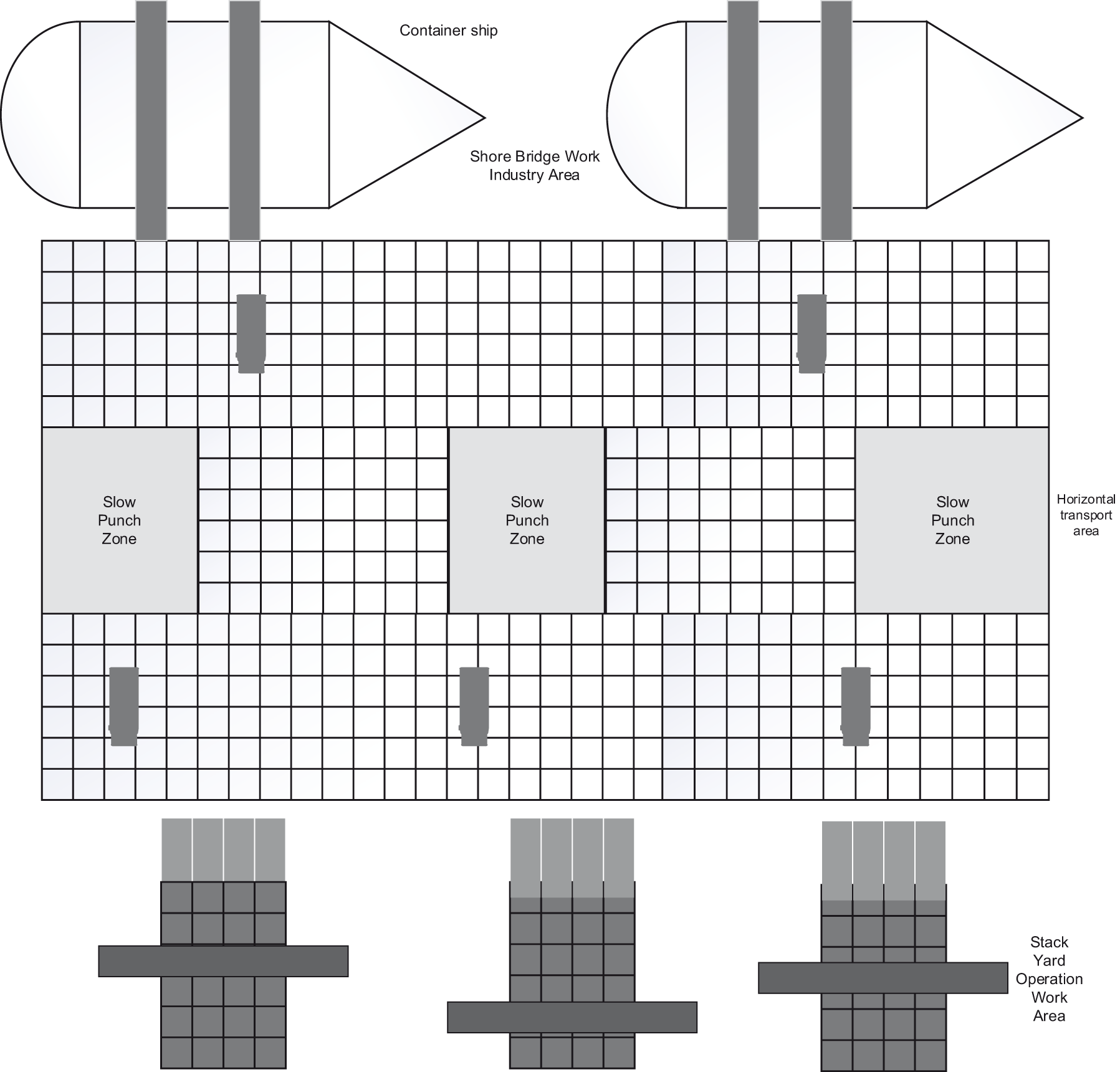
Figure 1: The layout of automated container terminals

The automated terminal’s AGV path planning system is a sophisticated system made up of numerous components, including shore bridges, yards, buffer zones, magnetic pegs, etc. The AGV horizontal transport area is taken into consideration, and the map is modeled using the grid method. Cells are used to represent the obstacle information of the AGV horizontal transport area, and their weights are Boolean variables where passable nodes are represented by 0 and impassable nodes by 1. The obstacle cells and the AGV cannot overlap.

2.2 Communication Interaction Protocols

A centralized control strategy is employed to discover a solution for all AGVs using a single central processing unit for horizontal transport operations at terminals with changeable surroundings. A wireless communication system, such as a communication interaction protocol between AGVs and the console, is required to implement communication between AGVs due to their constant movement and variety of horizontal transport tasks. The AGV sends the task starting point, the task deadline, and the following task receipt. Then, the AGV communicates the task start point, task finish point, and AGV cart number to the console, which then sends each cart the determined conflict-free path. This paper chooses user datagram protocol (UDP) wireless network communication, sets the network IP addresses of the AGV and console in the same IP network segment, and uses a wireless Wi-Fi signal to connect to the router to realize the communication between them while taking the cost of communication and the convenience of task operation into account. In the four corners and the center, a total of five WiFi access points (APs) are placed, using dual-band (2.4 and 5 GHz) APs, and installed at a height of 2–3 m above the ground to achieve complete WiFi coverage.

2.3 Multi-AGV Conflict Avoidance Strategy

1. Intersection conflict;

The intersection conflict is produced, as seen in Fig. 2a, when AGVi,AGVj move vertically toward the intersecting grid Vm and reach the same grid point Vm at once at time point t. Add constraints (AGVi,Vm,t) for AGVi and (AGVj,Vm,t) for AGVj, respectively, to this conflict binary tree node and treat it as a point conflict (AGVi,AGVj,Vm,t).

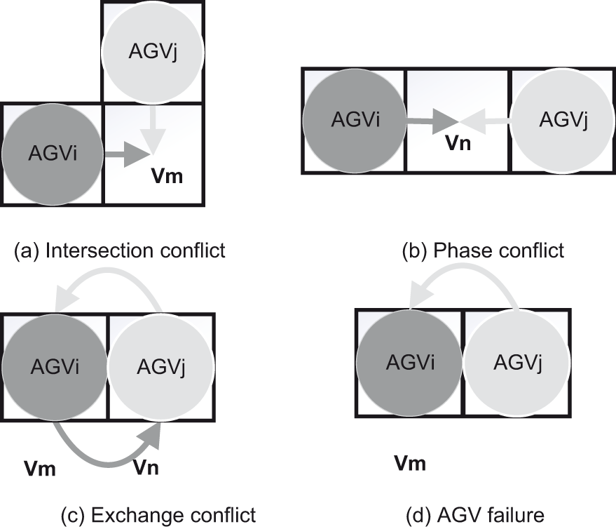
Figure 2: AGV main conflict types (a) intersection conflict; (b) phase conflict; (c) exchange conflict; (d) AGV failure

2. Phase conflict;

A phase conflict develops when AGVi and AGVj travel to the same grid node Vn from opposing directions and arrive at the same grid point Vn at the same time at time point t, as shown in Fig. 2b. As with the intersection conflict, it is referred to as a point conflict (AGVi,AGVj,Vn,t) and constraints are added to AGVi(AGVi,Vn,t) and AGVj(AGVj,Vn,t) on the conflict binary tree nodes, respectively.

3. Exchange conflict;

As seen in Fig. 2c, an exchange conflict occurs when AGVi, AGVj move in opposite directions to exchange the positions of grid points Vm, Vn at time point t. Think of it as an edge conflict (AGVi,AGVj,Vm,Vn,t), and apply constraints toAGVi(AGVi,Vm,Vn,t) and AGVj(AGVj,Vm,Vn,t) on the conflict binary tree nodes, respectively.

4. AGV failure.

As seen in Fig. 2d, the equipment must wait while the faulty AGVi stops at the grid point Vm and the planned path AGVj crosses the fault point. This model does not take into account the possibility of an AGV conflict due to a fault.

On the automated terminal, both point conflicts and edge conflicts occur. After determining the shortest path for each AGV using the Manhattan distance-based A * algorithm, the search proceeds on the conflict binomial tree. AGV mobility is constrained by each node on the conflict tree, comprising a set of constraints (N.constraints), a solution (N.solution), and a total cost (N.cost).

Fig. 3 illustrates an instance of AGV conflict at the terminal. Each AGV must plan its entire route from the shore bridge to the stacking yard. In the diagram, and represent two shore bridges S1 and S2, while G1 and G2 denote two stacking areas. Both AGVs’ routes have lengths of 3: AGV1:S1,A1,D,G1;AGV2:S2,B1,D,G2. They simultaneously reach grid point D at time step t2, resulting in a conflict. The decision AGV1 is for to wait until a certain time point, and the AGV with the shortest total path length is designated to apply the restriction. Consequently, N.solution = 7 emerges as the optimal solution in this scenario.

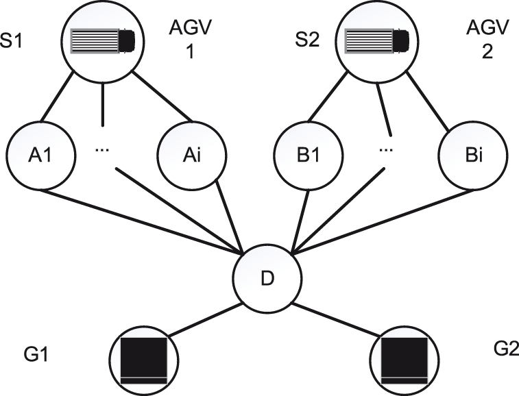
Figure 3: AGV conflict example

Fig. 4 displays the related conflict binary tree. The initial paths of AGV1 and AGV2 from the shore bridge to the heap and the yard are calculated using the underlying A* algorithm as N.solution={AGV1:S1,A1,D,G1},{AGV2:S2,B1,D,G2}; this results in N.cost = 6. The root node of the conflict tree corresponds to an empty constraint set, denoted as N.constraints={ϕ}. The root node is where this data is kept. A conflict (AGV1,AGV2,D,t2) occurs when both AGVs arrive at the raster point D at the time t2 during the verification of the supplied solution. Hence, the target node is not the root node.

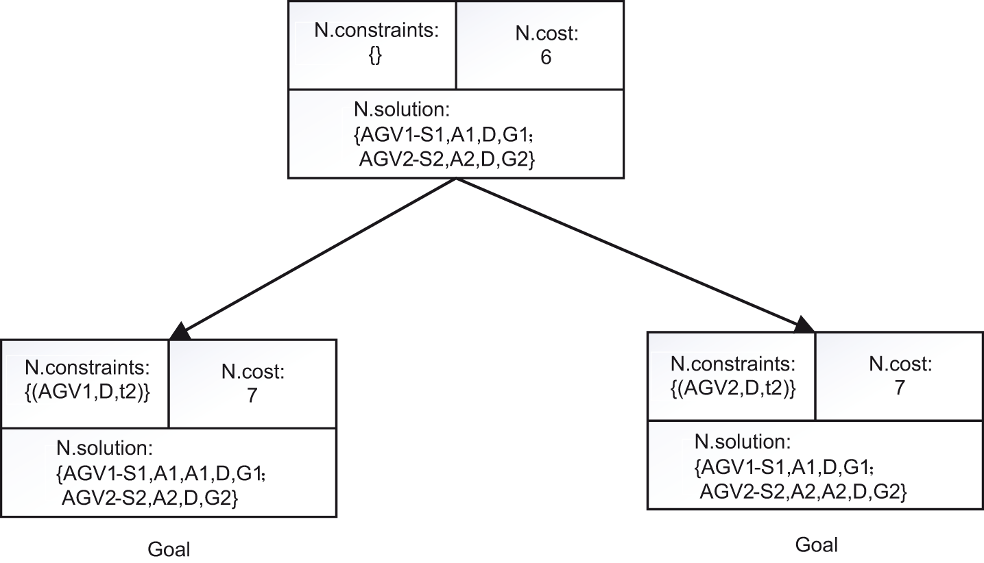
Figure 4: Conflict tree example

Two new child nodes are created to resolve the dispute. In contrast to the right child node, which adds constraints N.constraints={(AGV2,D,t2)}, the left child node adds constraints N.constraints={(AGV1,D,t2)}. To determine the best path while adhering to the new constraint, the left child node’s underlying A* search is invoked. To execute this, AGV1 must wait for a time point at A1 or S1, after which its new path becomes: {S1,A1,A1,D,G1}, whereas AGV2’s path in the left child node remains unchanged. The total cost for the left child node N.cost is 7.

Similarly, in creating the appropriate child node, the cost for Node N is 7. The OPEN node contains both child nodes. The left child node, which exhibits the lowest cost, is selected for expansion in the subsequent iteration of the while loop, confirming the underlying path. The left child node is identified as the target node because no conflict exists, making its solution N.solution the optimal one for this particular dock conflict case.

3  Mathematical Model

3.1 Assumptions

1. The shore bridge and yard are located in a fixed and well-known location, and there is one shore bridge for each section of the yard box;

2. Every AGV has an identical type definition;

3. The AGV runs at a steady pace, even while turning;

4. Without taking into account the impact of variables like failure, weather, and electricity while AGVs are being driven;

5. The idle AGV parking space is built up as a static obstruction in the buffer zone between the shore bridge and the yard, making it impossible for the AGV to move through when performing horizontal transportation operations;

6. AGVs can load and unload containers quickly between the yard and the beach bridge;

7. Every AGV grid route is accessible from both directions;

8. Several AGVs may be permitted to occupy the grid at the shore bridge, but only one AGV is permitted to occupy each grid at any time point.

3.2 Variable Setting

In representing the path network of AGVs in the horizontal transport area of the automated terminal, the path network of AGVs is represented by the G=(V,E,ob) directed weighted graph. where V denotes the set of all node numbers of the AGV grid graph on the automated terminal, V=[(x1,y1),(x2,y2),…,(xn,yn)], where n×n denotes the number of grids, and E is the set of edges of V, which denotes the length corresponding to each V. obdenotes the set of obstacle coordinates ob=[(xm,y1),(xm,y2),…,(xm,yn)]. Other variables are set as shown in Table 1.

3.3 Variable Setting

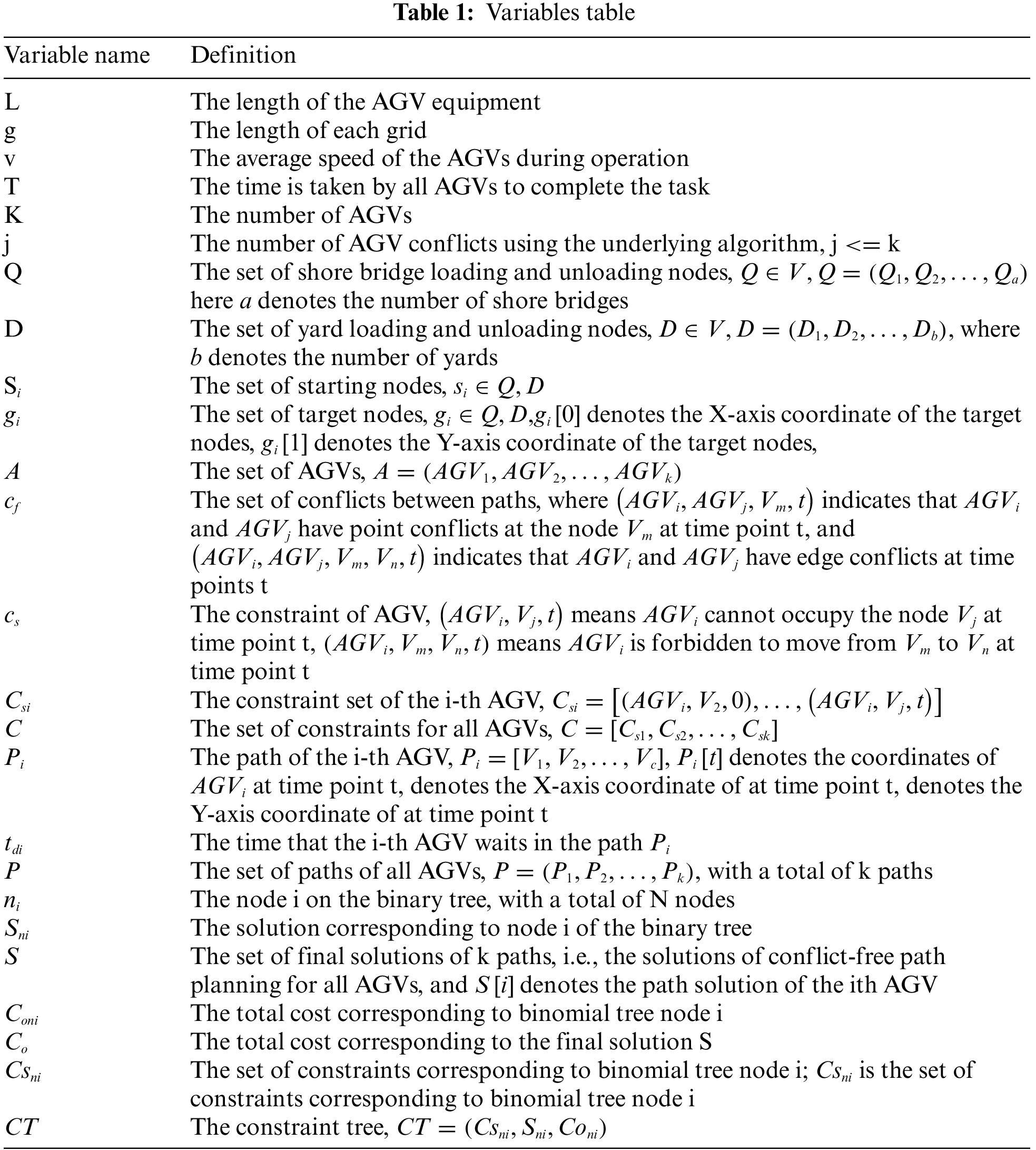
They should also be separated from the surrounding text by one space.

Objective function:

min∑i=1NConi(1)

Constraints:

Xij={1,AGVa accesses node j after accessing node i0,Otherwise}(2)

∑i=1N∑j=1NXij=1(3)

T=Cov(4)

f(i)=g(i)+h(i)(5)

h(i)=|Pi[ t ][ 0 ]−gi[ 0 ]|+|Pi[ t ][ 1 ]−gi[ 1 ]|(6)

Td=∑i=1ktdi(7)

mov={1,Indicates that the AGV is waiting in place0,Otherwise}(8)

Co=∑i=1kPi−1(9)

Eq. (1) indicates that the objective function of this model is the total cost minimization, Eqs. (2) and (3) indicates that each node is visited by AGV at most once at the same time, Eq. (4) indicates the time for all AGVs to complete the task, Eq. (5) indicates the A* algorithm used at the bottom, where f(i) is the estimation function, g(i) is the actual cost from the starting node to node i, h(i) is the estimated node i to the target node cost, Eq. (6) denotes the heuristic function using the Manhattan distance-based A* algorithm, Eq. (7) denotes the total waiting time, Eq. (8) denotes the choice of movement method for the AGVs, including waiting in place or moving one time step to a neighboring node, and Eq. (9) denotes the total cost of all AGVs to complete the task.

4  An Improved Bounded Conflicted-Based Search Algorithm on Automated Container Terminals

The solutions to MAPF problems are divided into two main categories: optimal solvers and suboptimal solvers. Optimal solvers work better when the number of AGVs is small, but as the number of AGVs increases, the state space grows exponentially, making finding the optimal solution NP-hard. However, in the case of AGV path planning on the automated terminal studied in this paper, with large map size and numerous AGVs, optimal solvers are not viable. Suboptimal solvers, known for their rapid solving speed, are usually preferred in scenarios involving a high number of AGVs.

Optimal solvers and suboptimal solvers constitute the primary solutions for MAPF issues. Finding the best solution for the MAPF problem is NP-hard because optimal solvers perform better with a low number of AGVs, but as the number grows, the state space expands exponentially. Unfortunately, due to the enormous map area and high AGV density in the automated terminal analyzed in this paper, optimal solvers cannot be applied. The swift-solving ability of suboptimal solvers makes them a popular choice in scenarios involving numerous AGVs.

This article employs the IBCBS algorithm, considering both point conflicts and determining edge conflicts in the binary tree. Furthermore, constraints are added to child nodes with edge conflicts to achieve multi-AGV conflict-free path planning. The utilization of focal search in both high-level and low-level tasks is employed to ensure solution quality while accelerating solution times.

The IBCBS algorithm flowchart is shown in Fig. 5, the left is a high level search and the right is a low-level single A* search. There are two lists of nodes in focal search which include Open_list and Focal_list. Open_list is a regular Open_list of A*. Focal_list is a subset of Open_list. The focal search uses two functions f1 and f2, f1 defines where nodes are in Focal_list and f2 defines which node from Focal_list to expand.

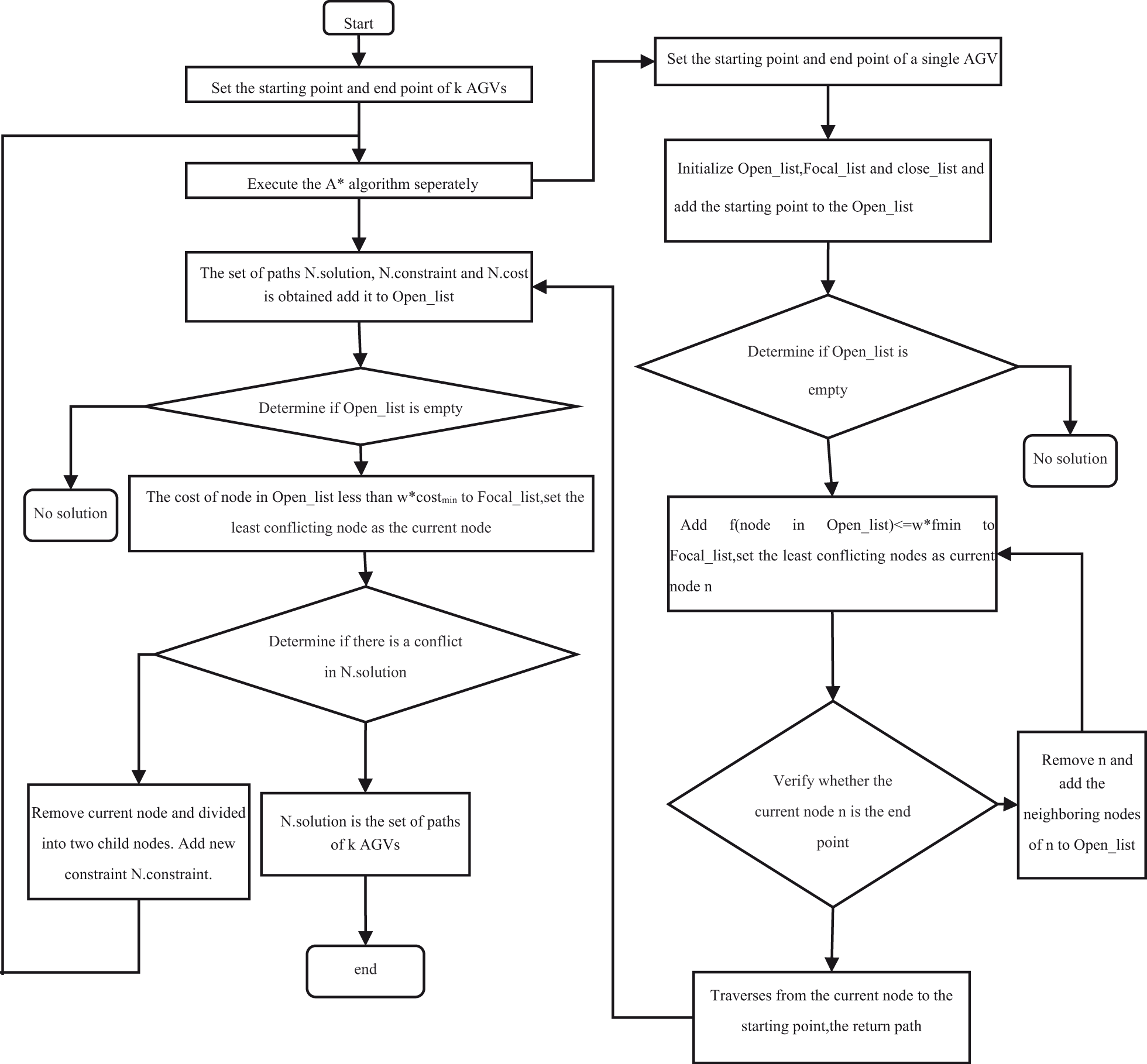
Figure 5: IBCBS algorithm flowchart

After setting start points and endpoints, conducted a single A* search for each agent to get paths. At the low-level of IBCBS, apply focal search (f,hc) for single AGV pathfinding where f(n) is the regular f(n)=g(n)+h(n), h(n) is the number of conflicts. At the high-level of IBCBS, search a binary tree called CT. Each node N in the tree consists of N.constraints, N.solution and N.cost. Each constraint belongs to an AGV and the root of CT is an empty set. There are k conflict-free paths in the solution and consistent with constraints. N.cost is the sum of all the paths. Apply focal search (g,hc) to search the CT, where g(n) is the cost of the CT node n and hc(n) is the number of conflicts. Determined no conflict in the locations reserved in all agents at all time steps and if no two AGVs plan to be at the same location at the same time, the paths are the solution. If a conflict exists, add a constraint to the CT node, and the low-level invoke again.

4.1 The Quality of the Solution

IBCBS(ωH,ωL) denote IBCBS uses ωH in high level and ωL in low level. IBCBS(ω,1) is a special case that focal search only used at a high level and IBCBS(1,ω) is focal search only used at a low level. The cost of IBCBS(ωH,ωL) is at most ωH∗ωL∗C∗. This also proves the boundedness of the algorithm.

4.2 The Completeness of the Algorithm

The expansion cost of both IBCBS is no more than ω times higher than the ideal solution. Moreover, within OPEN, at least one CT node consistently aligns with every viable answer. Due to its systematic search, it eventually identifies all solutions. Consequently, IBCBS concludes.

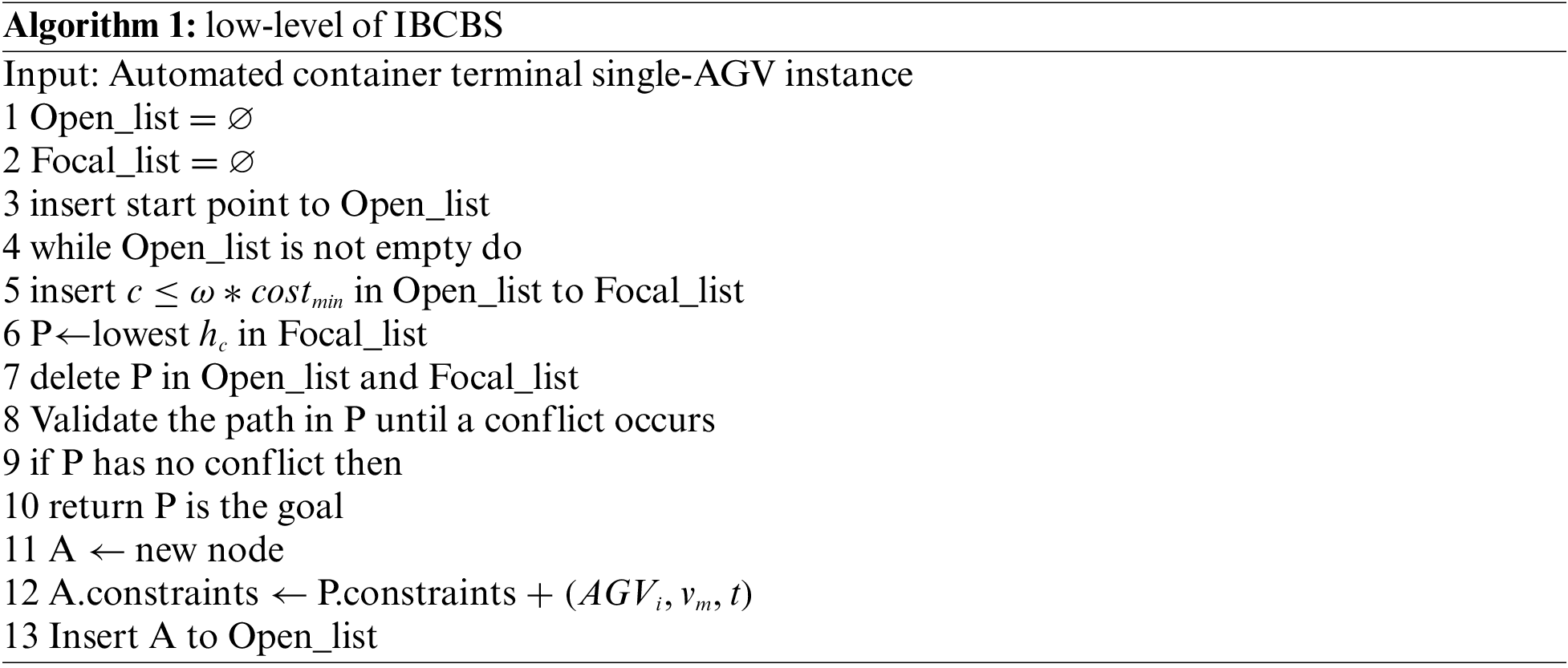
Algorithm 1 presents the pseudo-code for a low level of IBCBS which uses a Manhattan distance-based A* algorithm with focal search (f,hc) for each single AGV path planning.

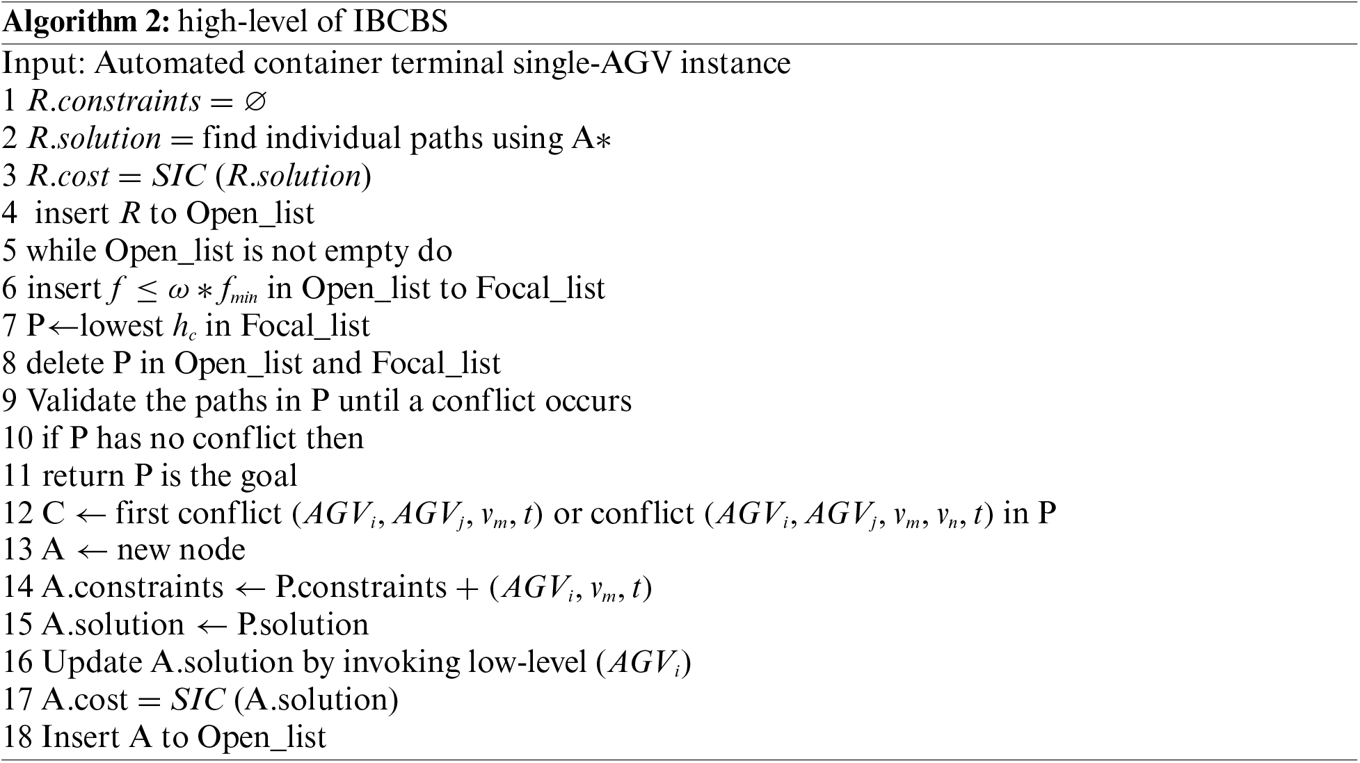
Algorithm 2 presents the pseudo-code for a high level of IBCBS which use focal-search (g,hc) to choose the cost of nodes in CT lower than ω∗g.

5  Experimental Results and Analysis

Referring to the actual situation of the automated terminal, a two-way grid road network diagram is designed, as depicted in Fig. 6. In the road network layout, Q1–Q10 represents the location of the quay crane, while D1–D30 signifies the location of the container yard. The white grid denotes an access point, whereas the grey indicates a static obstacle that is inaccessible. The program is written in Python and runs on an Intel® AMD5-2500U CPU @ 2.00 GHz with 8 GB memory on a Windows 10 computer.

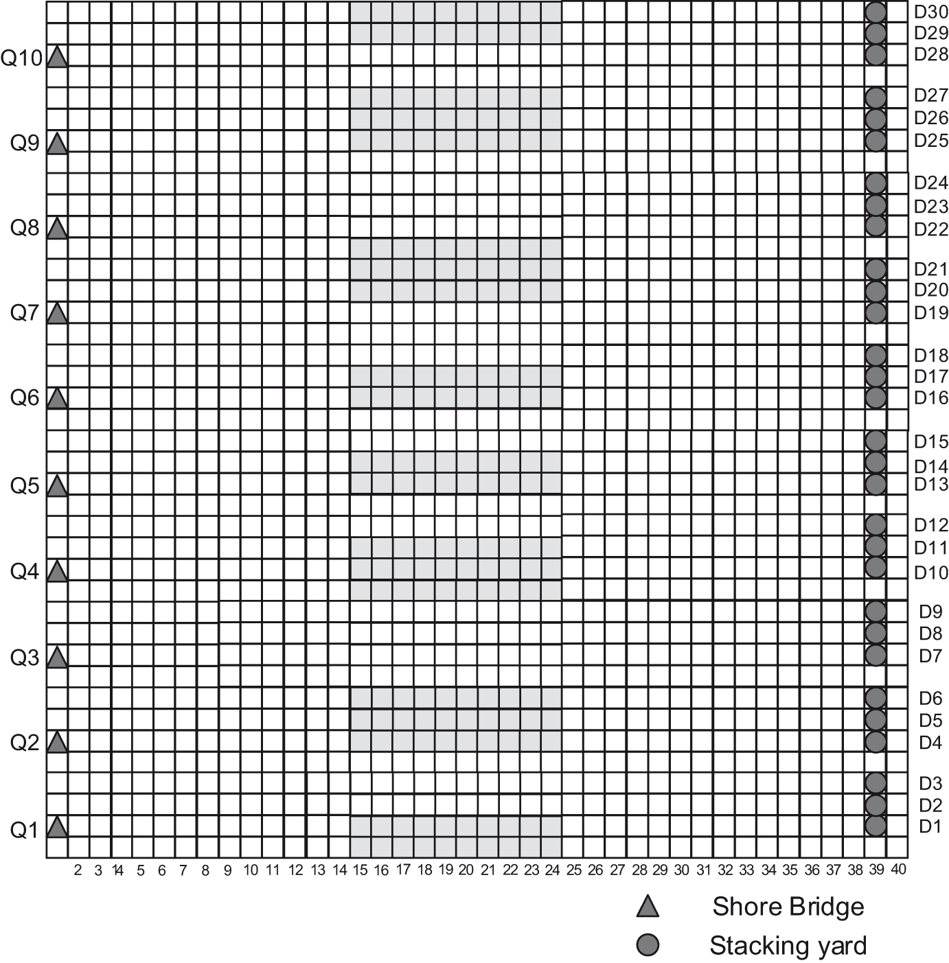
Figure 6: AGV road network layout

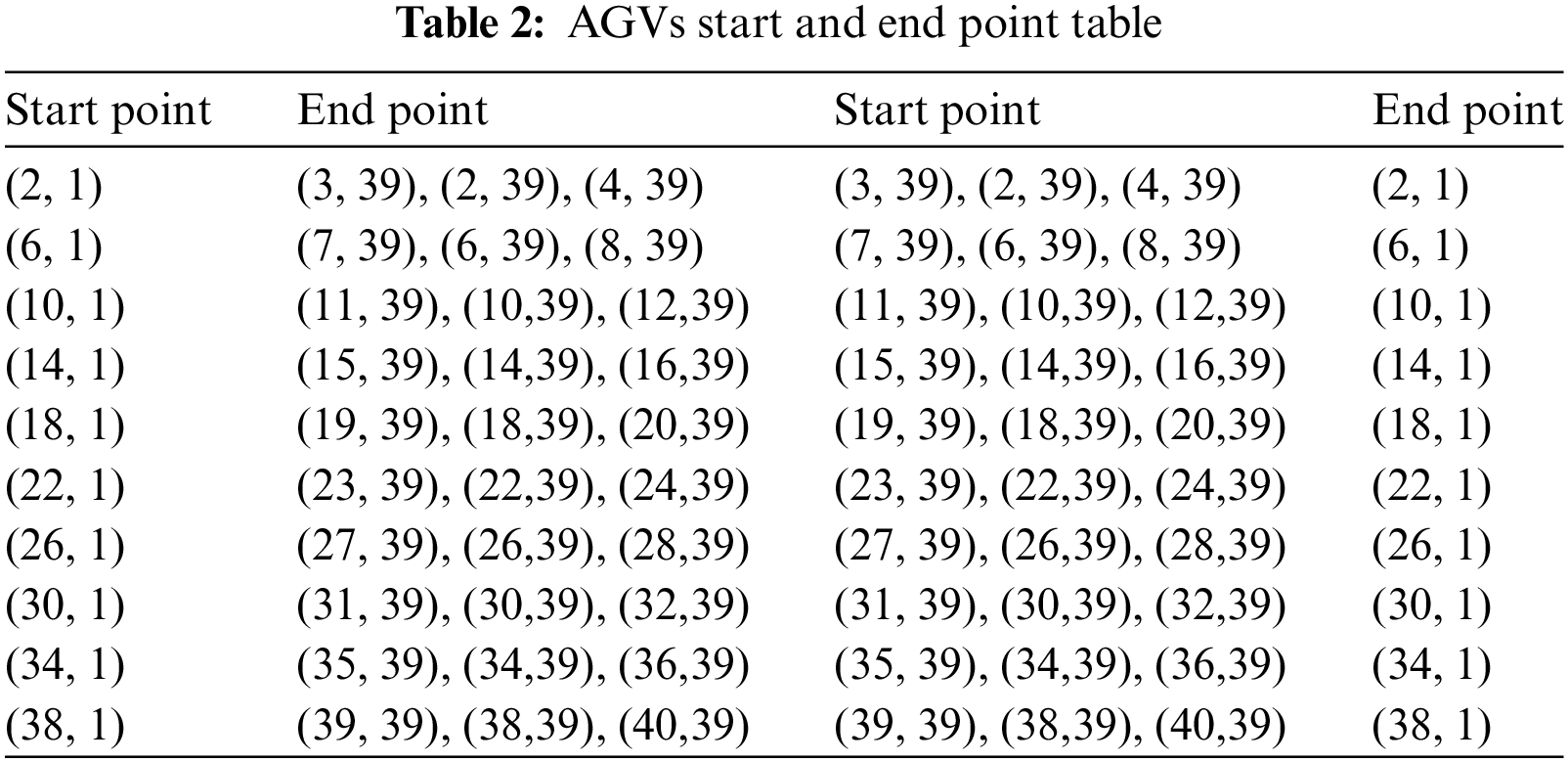
The following criteria are utilized in this example: The AGV road network size is set to 40 × 40 with a grid length of 2 m. The starting point and endpoint information can be found in Table 2. Both the starting point and endpoint are selected according to the operating mode, either from the shore bridge to the container yard or from the container yard to the shore bridge. Each AGV maintains a constant speed of 2 m/s, with a length of 2 m.

5.1 Performance Comparison Experiments between CBS and IBCBS Algorithms for Different Numbers of AGVs with Starting Endpoints

Set the number of AGVs as 10, 20, 30, 40, 50, and 60, and then randomly select the starting and endpoint based on Table 1. The shore bridge can be repeatedly selected. For AGV = 10, 20, 30, the starting point includes all shore bridges, and the endpoint is the yard. For AGV = 30, the endpoint includes all yards. However, for AGV = 40, 50, 60, 30 units move from the shore bridge to the yard, while the others move from the yard to the shore bridge. The starting point and endpoint remain fixed after random selection.

Set ω = 1.1. Four methods—IBCBS (ω, 1), IBCBS (1, ω), IBCBS (ω,ω) and CBS—are utilized for 100 experiments each. The effective time is set to 60 s, and if a solution cannot be obtained within this time, it is considered as unsolvable. Despite fixing the number of AGVs and algorithms, the computing time for each experiment differs while maintaining the same total path length. Thus, the computing time for 2400 experiments is depicted in Fig. 7.

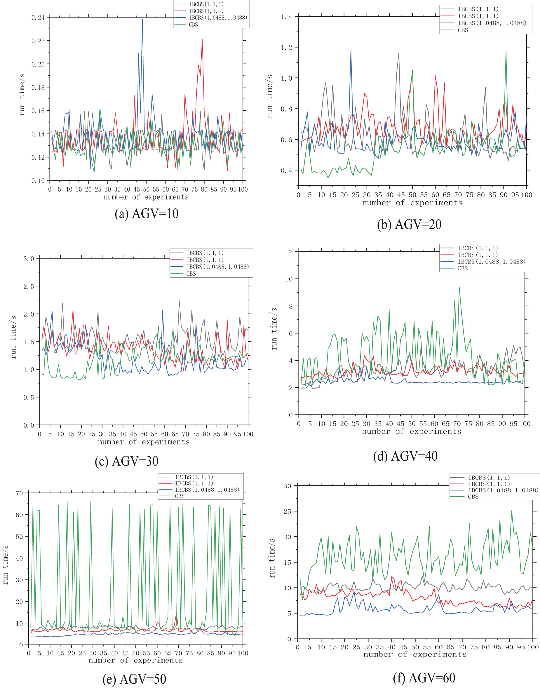
Figure 7: Run time of IBCBS (ω, 1), IBCBS (1, ω), IBCBS (ω,ω) and CBS. (a) AGV = 10; (b) AGV = 20; (c) AGV = 30; (d) AGV = 40; (e) AGV = 50; (f) AGV = 60

It is evident from Fig. 7 that with a smaller AGV scale of 10, 20, 30, conflicts among AGVs are fewer. The effectiveness of focal search between the high-level and low-level in IBCBS is less pronounced. Additionally, the discrepancy between CBS and IBCBS (ω, 1), IBCBS (1, ω), IBCBS (ω,ω) is marginal. However, as the AGV scale increases to 40, 50, 60, AGV conflicts surge. IBCBS sacrifices optimality, leading to a slackening effect in both the high-level and low-level operations. Notably, CBS’s operational time is significantly longer compared to IBCBS (ω, 1), IBCBS (1, ω), IBCBS (ω,ω).

Fig. 8 illustrates that the effectiveness of bounded suboptimal search is not immediately evident with a low number of AGVs. Conflicts are minimal, below 30 units, resulting in comparable computing times for the six methods. However, as the AGV count exceeds 30 units, both point and edge conflicts rise, consequently escalating computing times for all six methods. The CBS algorithm consistently strives for optimal solutions, resulting in longer operational times. Due to convergence, GCBS algorithm operation times are extended, while BCBS operation times are marginally better than CBS and less than the other three IBCBS algorithms. The three IBCBS algorithms adopt focal search with different levels of permissive optimality constraints, substantially reducing runtime and enhancing computational efficiency. Among them, IBCBS (1.0488, 1.0488) uses focal search at both high and low levels, exhibiting the shortest operational time.

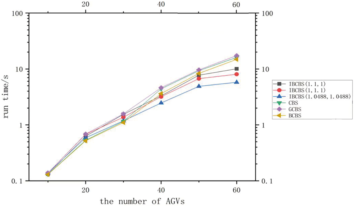
Figure 8: Average run time of IBCBS (ω, 1), IBCBS (1, ω), IBCBS (ω,ω), GCBS, BCBS and CBS, when the number of AGVs is 10, 20, 30, 40, 50, 60

Fig. 9 indicates that CBS consistently yields the shortest total path length regardless of AGV count, with IBCBS following as the second shortest. At 10 AGVs, where path conflicts are absent, the total path length is identical for all four methods. Even with an increased AGV count, the total path length of the three IBCBS methods cannot exceed 1.1 times that of CBS due to CBS’s optimal nature, resulting in the shortest total path length. IBCBS is constrained by *cost, set at 1.1. By incorporating additional measures at the low level, potential conflicts can be averted. Consequently, IBCBS (1, 1) displays a shorter path length than IBCBS (1.0488, 1.0488) and IBCBS (1.1, 1).

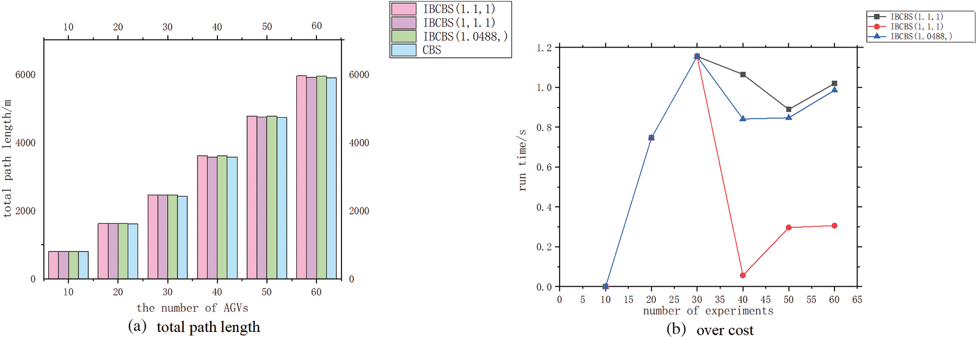
Figure 9: When the number of AGVs is 10, 20, 30, 40, 50, 60, (a) total path length (b) over the cost of IBCBS (ω, 1), IBCBS (1, ω), IBCBS (ω,ω) and CBS

Table 3 presents specific experimental data. The reduced time is calculated as (CBS’s average run time-IBCBS’s average run time)/CBS’s average run time, expressed as a percentage. Meanwhile, the over cost is determined by (IBCBS’s total path length-CBS’s total path length)/CBS’s total path length, also as a percentage. The results indicate that, in line with the analyses in Figs. 7 and 8, CBS exhibits the lowest operation time at AGV = 10, 20, 30; whereas, at AGV = 40, 50, 60, IBCBS (1.0488, 1.0488) demonstrates the lowest time, reduced by up to 64.06%. Regarding the total path length, as observed in Fig. 9, the sequence from shortest to longest is CBS, IBCBS (1, 1.1), IBCBS (1.0488, 1.0488), IBCBS (1.1, 1). All variants of IBCBS maintain an over the cost of no more than 1.2%.

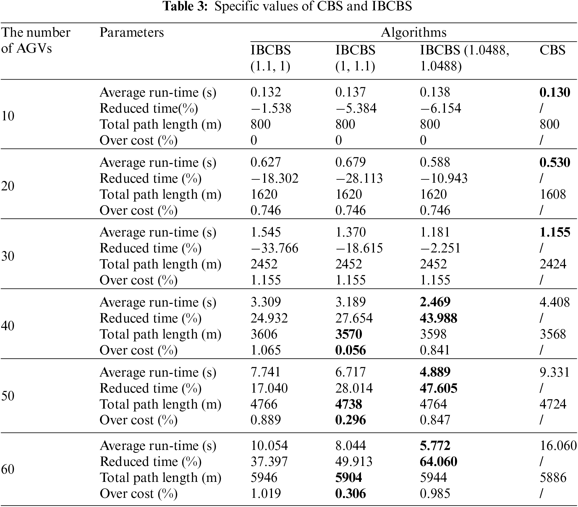
Based on the analysis, when a low total path length is desired, the CBS algorithm is automatically preferred. For fewer AGVs (10, 20, or 30), CBS stands as the best choice due to its shorter computation time and total path length. On the other hand, when more AGVs are involved (40, 50, or 60), the IBCBS algorithm becomes the selection due to its shorter computation time and its ability to accept a more costly solution (1.0488, 1.0488).

5.2 Performance Comparison Experiments of Three IBCBS Algorithms with Randomly Selected Starting Endpoints

AGV counts were set to 10, 20, 30, 40, 50, and 60, with starting and ending points chosen randomly from Table 1. The shore bridge can be selected repeatedly, without considering potential conflicts. For AGV = 10, 20, 30, the starting and ending points are selected from the shore bridge to the yard. For AGV = 40, 50, 60, 30 units are chosen from the shore bridge to the yard, while the remaining units are from the yard to the shore bridge.

In Fig. 10, a horizontal comparison highlights that as the number of AGVs increases, conflicts intensify, resulting in fewer valid points and declining success rates across all three algorithms. However, with the same AGV count, employing focal searches at the high level extends the search range and enhances the success rate, leading to an increased number of green points. These green points surpass the red and blue ones because only IBCBS (1, 1.1) and IBCBS (1.0488, 1.0488), which conduct focal search solely at the low level, might avoid potential conflicts and exhibit lower operation times.

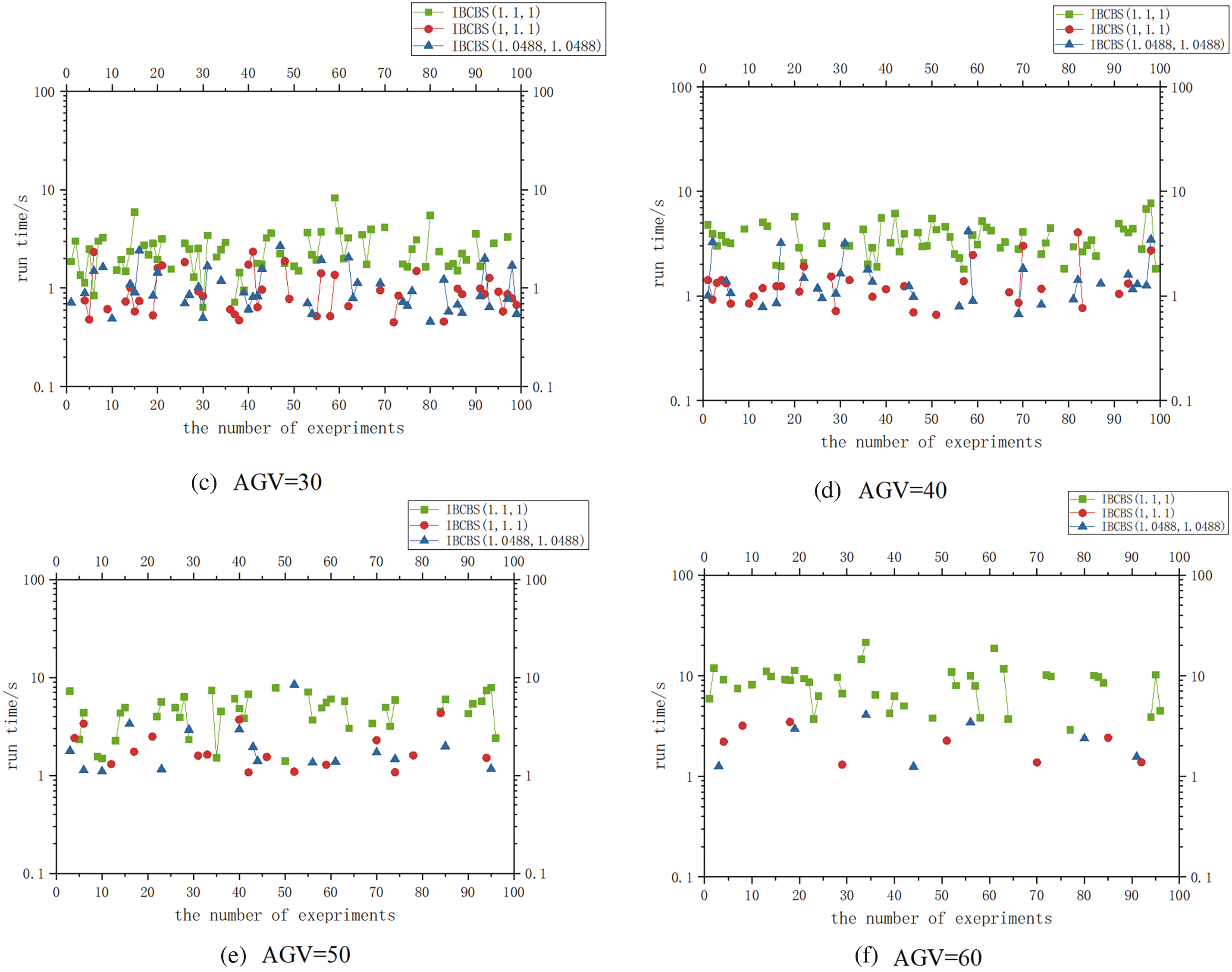
Figure 10: Run time of IBCBS (ω, 1), IBCBS (1, ω) and IBCBS (ω,ω). (a) AGV = 10; (b) AGV = 20; (c) AGV = 30;(d) AGV = 40;(e) AGV = 50; (f) AGV = 60

Fig. 11, following the analysis from Fig. 10, displays the average run times of the three algorithms across 100 experiments. As the number of AGVs increases, all three algorithms take longer to compute. Notably, IBCBS (1.1, 1) takes significantly more time than IBCBS (1, 1.1) and IBCBS (1.0488, 1.0488). However, IBCBS (1.0488, 1.0488) exhibits the fastest operation time, employing focal search at both top and bottom levels, encompassing a wider search range.

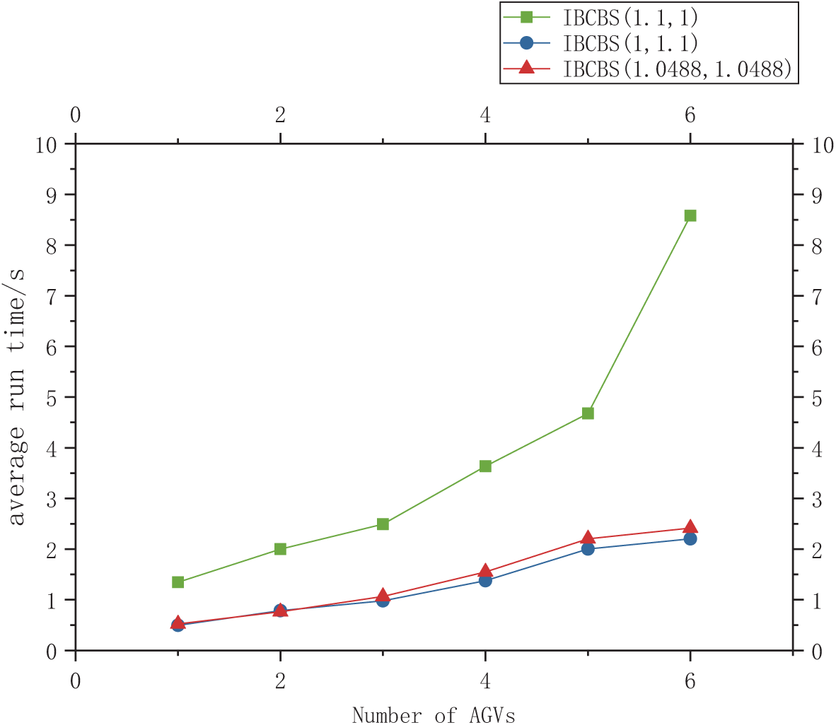
Figure 11: Average run time of three kinds of IBCBS

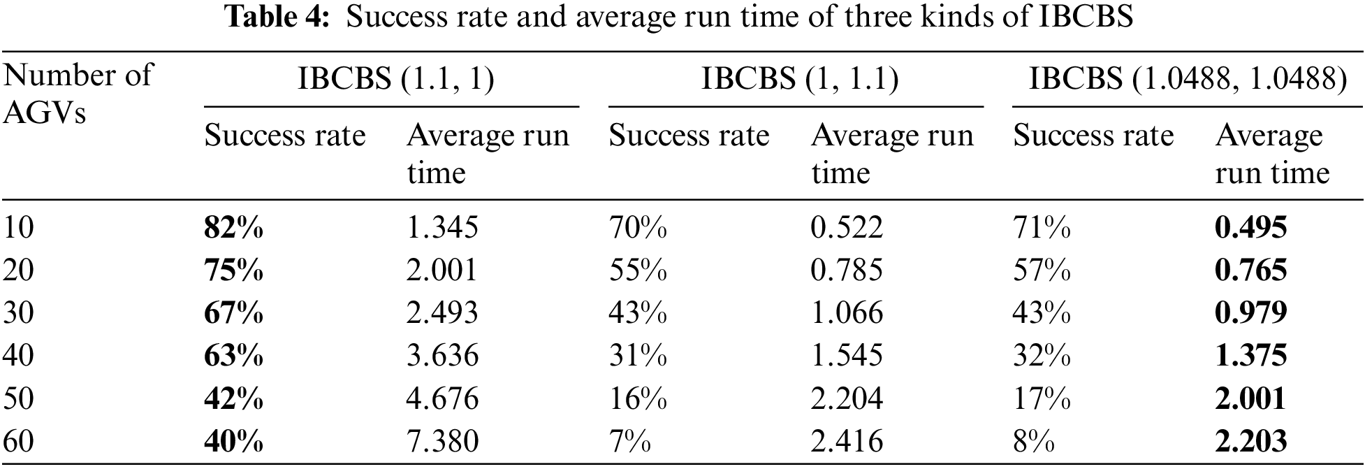
Table 4 demonstrates specific success rates and average operation times using the three algorithms after randomly choosing starting and ending points. Based on the analysis, IBCBS (1.1, 1) attains the highest success rate among the three algorithms, while IBCBS (1.0488, 1.0488) records the shortest operation time. If the problem model prioritizes a higher success rate over operation time, selecting IBCBS (1.1, 1) is recommended, despite its longer operation time. Conversely, if a higher operation time is required, choosing IBCBS (1.0488, 1.0488) would be preferable.

5.3 Experimental Analysis of the Value of ω in IBCBS (ω, 1) on the Performance When AGV = 60 Units

Set the effective time limit at 60 s, beyond which the solution is considered invalid. Choose 60 AGVs, with half of them moving from the shore bridge to the yard and the other half from the yard to the shore bridge. Fix the values at 1.01, 1.05, 1.1, 1.5, and 2.0 for ω, and opt for IBCBS (ω, 1) with the highest success rate among the three methods. Conduct 100 experiments.

Fig. 12 depicts the computing time for 500 experiments, where times exceeding 60 s are deemed invalid. Experiment configurations, particularly the starting and endpoint selections, are random, occasionally resulting in computing times surpassing the limit. For instance, at ω = 1.01 and 1.05, some instances exceed 60 s, while other data cluster around 7.0 s. At ω = 1.01, the operation takes longer (illustrated by the green squares), with fewer instances indicating the lowest success rate compared to other data.

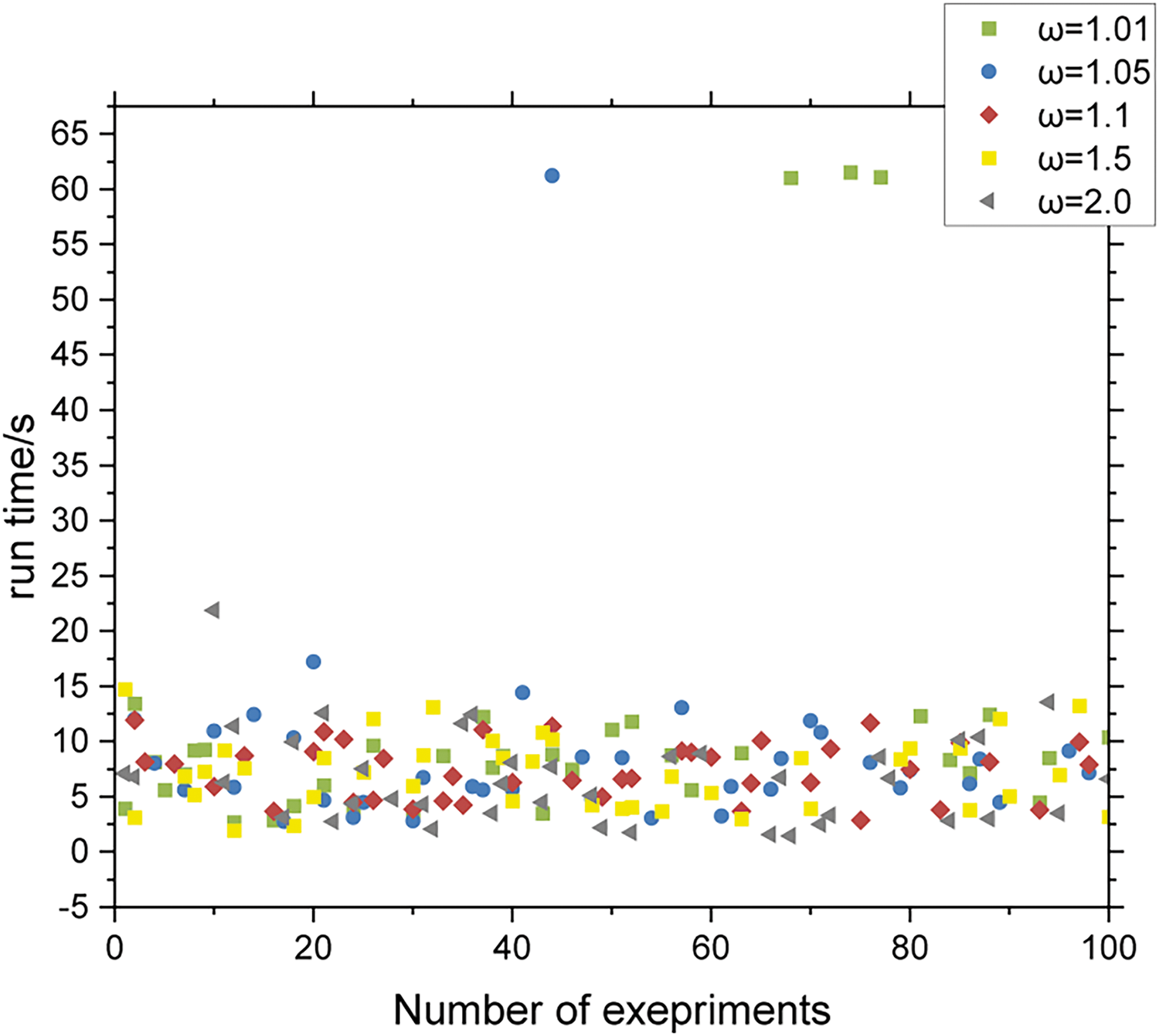
Figure 12: Run time of IBCBS (1.01, 1), IBCBS (1.05, 1), IBCBS (1.1, 1), IBCBS (1.5, 1) and IBCBS (2.0, 1)

Fig. 13 displays the average operation time and success rate, excluding invalid data where operation times exceeded 60 s. With smaller ω values, the focal search scope decreases, making it challenging to find valid solutions through Focal_list traversal. Therefore, success rates rise and average run times decline as ω increases from 1.01 to 1.05 and 1.1. As ω grows larger, the Focal_list node count increases, enhancing the chance of the target node’s existence. Beyond ω = 1.1, the success rate plateaus, yet increasing ω widens the search range, enabling faster discovery of nodes with fewer conflicts, thereby enhancing algorithm efficiency.

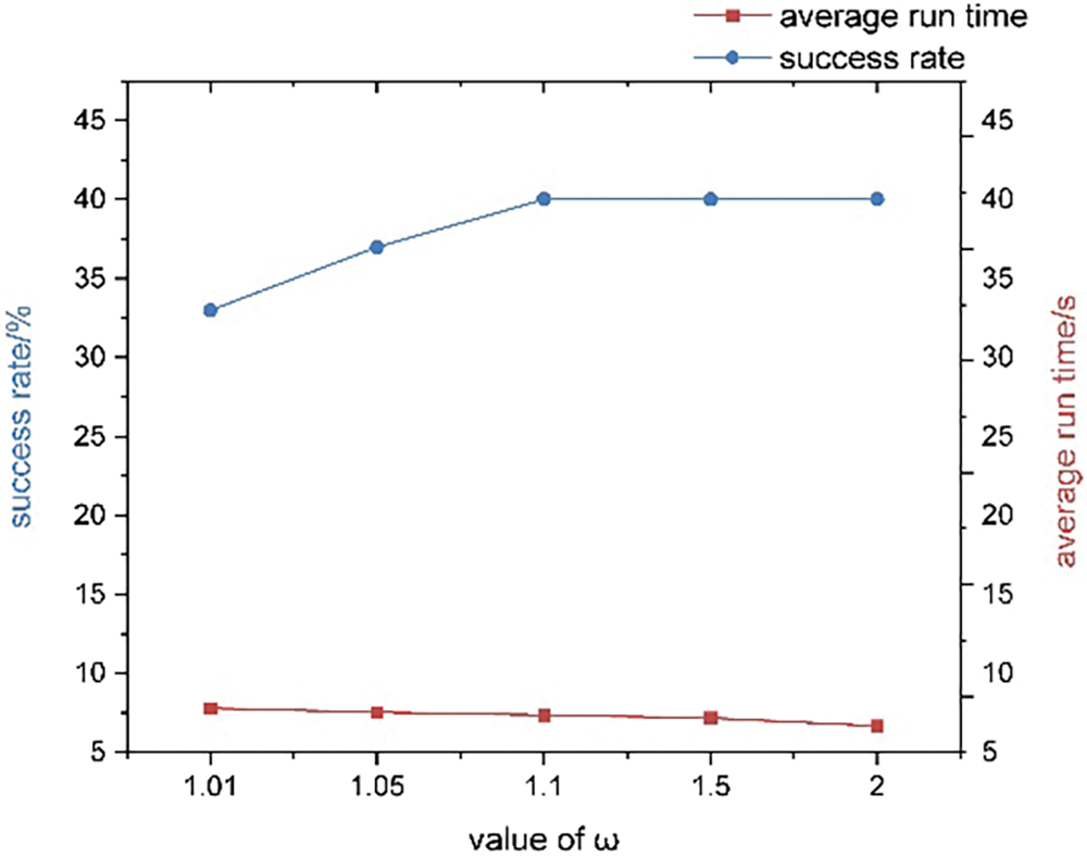
Figure 13: Success rate and average run time of IBCBS (ω, 1)

Table 5 presents specific success rates and average operation time data for varying ω values in IBCBS (ω, 1). Based on the analysis, when dealing with 60 AGVs in the automated terminal, ω = 2.0 is preferable for high success rates and rapid computing times, whereas ω = 1.1 is preferable for maintaining a high success rate with excellent solution quality.

6  Conclusions

To enhance productivity and minimize conflicts, a novel bounded conflict-based search method was introduced for ACT. Addressing AGV point and edge conflicts, the approach aimed to minimize AGVs’ total path length. We developed a multi-AGV conflict-free path planning model and solved it using the IBCBS algorithm with focal search. Our study compared the efficiency of IBCBS and CBS algorithms through several numerical experiments. The comparison was conducted across four techniques involving varying AGV numbers in three sets of experiments. Initially, with fixed start and endpoints and ω value set at 1.1, all three IBCBS algorithms outperformed CBS. At 30 to 60 AGVs, IBCBS (1.0488, 1.0488) exhibited the highest speed and maintained an over cost of no more than 1.2%. Subsequently, employing randomly selected start and endpoints demonstrated the swiftness of IBCBS (1.0488, 1.0488) and the higher success rate of IBCBS (1.1, 1). Finally, using the IBCBS (ω, 1) algorithm revealed a higher success rate with ω above 1.1 and shorter average run times specifically at ω = 2.0. Our experiments indicate the practical applicability of the proposed IBCBS algorithm to existing automatic terminals, promising a significant enhancement in efficiency.

In our study, AGV speed remained constant. However, in practical scenarios, AGV speed might decrease or halt during turns or malfunctions. Future work could consider increasing the turning factor to minimize turns and better reflect real ACT scenarios. Additionally, employing reinforcement learning in future studies might further enhance solution speed.

Acknowledgement: The authors would like to acknowledge that this work would not have been possible without the support of the Shanghai Maritime University.

Funding Statement: This work was supported by National Natural Science Foundation of China (No. 62073212), Shanghai Science and Technology Commission (No. 23ZR1426600).

Author Contributions: Xinci Zhou: Methodology, Software, Validation, Investigation, Resources, Writing original draft, Visualization; Jin Zhu: Conceptualization, Formal analysis, Writing—review and editing, Supervision, Project administration, Funding acquisition.

Availability of Data and Materials: All the reviewed research literature and used data in this research paper consists of publicly available scholarly articles, conference proceedings, books, and reports. The references and citations are contained in the reference list of this manuscript and can be accessed through online databases, academic libraries, or by contacting the respective publishers.

Conflicts of Interest: The authors declare that they have no conflicts of interest to report regarding the present study.

References

1. Zhang, Z., Chen, J., Guo, Q. (2023). Application of automated guided vehicles in smart automated warehouse systems: A survey. Computer Modeling in Engineering & Sciences, 134(3), 1529–1563. https://doi.org/10.32604/cmes.2022.021451 [Google Scholar] [CrossRef]

2. Xu, C., Zhu, H., Zhu, H., Wang, J., Zhao, Q. (2023). Improved RRT ∗ algorithm for automatic charging robot obstacle avoidance path planning in complex environments. Computer Modeling in Engineering & Sciences, 137(3), 2567–2591. https://doi.org/10.32604/cmes.2023.029152 [Google Scholar] [CrossRef]

3. Yue, L., Fan, H. (2022). Dynamic scheduling and path planning of automated guided vehicles in automatic container terminal. IEEE/CAA Journal of Automatica Sinica, 9(11), 2005–2019. https://doi.org/10.1109/jas.2022.105950 [Google Scholar] [CrossRef]

4. Yuan, Z., Yang, Z., Lv, L., Shi, Y. (2020). A bi-level path planning algorithm for multi-AGV routing problem. Electronics, 9(9), 1351. https://doi.org/10.3390/electronics9091351 [Google Scholar] [CrossRef]

5. Wang, Y. J., Liu, X. Q., Leng, J. Y., Wang, J. J., Meng, Q. N. et al. (2022). Study on scheduling and path planning problems of multi-AGVs based on a heuristic algorithm in intelligent manufacturing workshop. Advances in Production Engineering & Management, 17(4), 505–513. https://doi.org/10.14743/apem2022.4.452 [Google Scholar] [CrossRef]

6. Fazlollahtabar, H., Hassanli, S. (2017). Hybrid cost and time path planning for multiple autonomous guided vehicles. Applied Intelligence, 48(2), 482–498. https://doi.org/10.1007/s10489-017-0997-x [Google Scholar] [CrossRef]

7. Draganjac, I., Miklic, D., Kovacic, Z., Vasiljevic, G., Bogdan, S. (2016). Decentralized control of multi-AGV systems in autonomous warehousing applications. IEEE Transactions on Automation Science and Engineering, 13(4), 1433–1447. https://doi.org/10.1109/tase.2016.2603781 [Google Scholar] [CrossRef]

8. Chen, J., Zhang, X., Peng, X., Xu, D., Peng, J. (2022). Efficient routing for multi-AGV based on optimized Ant-agent. Computers & Industrial Engineering, 167, 108042. https://doi.org/10.1016/j.cie.2022.108042 [Google Scholar] [CrossRef]

9. Li, J., Xu, B., Yang, Y., Wu, H. (2018). Quantum ant colony optimization algorithm for AGVs path planning based on Bloch coordinates of pheromones. Natural Computing, 19(4), 673–682. https://doi.org/10.1007/s11047-018-9711-0 [Google Scholar] [CrossRef]

10. Choi, H. B., Kim, J. B., Han, Y. H., Oh, S. W., Kim, K. (2022). MARL-based cooperative multi-AGV control in warehouse systems. IEEE Access, 10, 100478–100488. https://doi.org/10.1109/access.2022.3206537 [Google Scholar] [CrossRef]

11. Guo, K., Zhu, J., Shen, L. (2021). An improved acceleration method based on multi-agent system for AGVs conflict-free path planning in automated terminals. IEEE Access, 9, 3326–3338. https://doi.org/10.1109/access.2020.3047916 [Google Scholar] [CrossRef]

12. Hu, Y. J., Dong, L. C., Xu, L. (2020). Multi-AGV dispatching and routing problem based on a three-stage decomposition method. Mathematical Biosciences and Engineering, 17(5), 5150–5172. https://doi.org/10.3934/mbe.2020279 [Google Scholar] [PubMed] [CrossRef]

13. Zhong, M., Yang, Y., Dessouky, Y., Postolache, O. (2020). Multi-AGV scheduling for conflict-free path planning in automated container terminals. Computers & Industrial Engineering, 142, 106371. https://doi.org/10.1016/j.cie.2020.106371 [Google Scholar] [CrossRef]

14. Zhong, M., Yang, Y., Sun, S., Zhou, Y., Postolache, O. et al. (2020). Priority-based speed control strategy for automated guided vehicle path planning in automated container terminals. Transactions of the Institute of Measurement and Control, 42(16), 3079–3090. https://doi.org/10.1177/0142331220940110 [Google Scholar] [CrossRef]

15. Wang, J., Sun, Y., Zhang, Z., Gao, S. (2020). Solving multitrip pickup and delivery problem with time windows and manpower planning using multiobjective algorithms. IEEE/CAA Journal of Automatica Sinica, 7(4), 1134–1153. https://doi.org/10.1109/jas.2020.1003204 [Google Scholar] [CrossRef]

16. Luo, J., Wu, Y. (2015). Modelling of dual-cycle strategy for container storage and vehicle scheduling problems at automated container terminals. Transportation Research Part E: Logistics and Transportation Review, 79, 49–64. https://doi.org/10.1016/j.tre.2015.03.006 [Google Scholar] [CrossRef]

17. Ma, A., Ouimet, M., Cortés, J. (2020). Hierarchical reinforcement learning via dynamic subspace search for multi-agent planning. Autonomous Robots, 44(3–4), 485–503. https://doi.org/10.1007/s10514-019-09871-2 [Google Scholar] [CrossRef]

18. Zhou, Y., Yang, H., Wang, Y., Yan, X. (2021). Integrated line configuration and frequency determination with passenger path assignment in urban rail transit networks. Transportation Research Part B: Methodological, 145, 134–151. https://doi.org/10.1016/j.trb.2021.01.002 [Google Scholar] [CrossRef]

19. Chen, H., Chen, B., Varshney, P. K. (2012). A new framework for distributed detection with conditionally dependent observations. IEEE Transactions on Signal Processing, 60(3), 1409–1419. https://doi.org/10.1109/tsp.2011.2177975 [Google Scholar] [CrossRef]

20. Andreychuk, A., Yakovlev, K., Surynek, P., Atzmon, D., Stern, R. (2022). Multi-agent pathfinding with continuous time. Artificial Intelligence, 305(C). https://doi.org/10.1016/j.artint.2022.103662 [Google Scholar] [CrossRef]

21. Goldenberg, M., Felner, A., Stern, R., Sharon, G., Sturtevant, N. et al. (2014). Enhanced partial expansion A. Journal of Artificial Intelligence Research, 50, 141–187. https://doi.org/10.1613/jair.4171 [Google Scholar] [CrossRef]

22. Sharon, G., Stern, R., Goldenberg, M., Felner, A. (2013). The increasing cost tree search for optimal multi-agent pathfinding. Artificial Intelligence, 195, 470–495. https://doi.org/10.1016/j.artint.2012.11.006 [Google Scholar] [CrossRef]

23. Sharon, G., Stern, R., Felner, A., Sturtevant, N. R. (2015). Conflict-based search for optimal multi-agent pathfinding. Artificial Intelligence, 219, 40–66. https://doi.org/10.1016/j.artint.2014.11.006 [Google Scholar] [CrossRef]

24. Pearl, J., Kim, J. H. (1982). Studies in semi-admissible heuristics. IEEE Transactions on Pattern Analysis and Machine Intelligence, (4), 392–399. https://doi.org/10.1109/TPAMI.1982.4767270 [Google Scholar] [PubMed] [CrossRef]

25. Lifschitz, V. (2019). Answer set programming, pp. 1–147. Heidelberg: Springer. [Google Scholar]

26. Barer, M., Sharon, G., Stern, R., Felner, A. (2014). Suboptimal variants of the conflict-based search algorithm for the multi-agent pathfinding problem. Proceedings of the International Symposium on Combinatorial Search, 5, 19–27. https://doi.org/10.1609/socs.v5i1.18315 [Google Scholar] [CrossRef]