Decoupling Algorithms for the Gravitational Wave Spacecraft

1  Introduction

In 2016, the LIGO team in the United States announced the detection of gravitational waves. It was the first direct detection of gravitational waves in human history. To detect gravitational waves at lower frequencies, researchers have proposed space gravitational wave detection missions such as the Laser Interferometer Space Antenna (LISA) [1], Taiji [2] and TianQin [3]. Interest in this research field is steadily growing, with related studies spanning various aspects such as orbit [4], laser links [5], low-noise mechanisms [6], algorithms [7], and more. As shown in Fig. 1, the space gravitational wave detection formation consists of three identical spacecraft, each with two Moving Optical Assemblies (MOAs). Each MOA consists of an optical bench (OB), a telescope, and a test mass (TM) protected in the electrode cage. The three spacecraft form a triangular constellation with an interferometric arm between each two. Gravitational waves are detected by measuring the change in distance between two TMs on the same interferometric arm. The MOA can be driven to rotate around its pivot by the Optical Assembly Tracking Mechanism (OATM) [8].

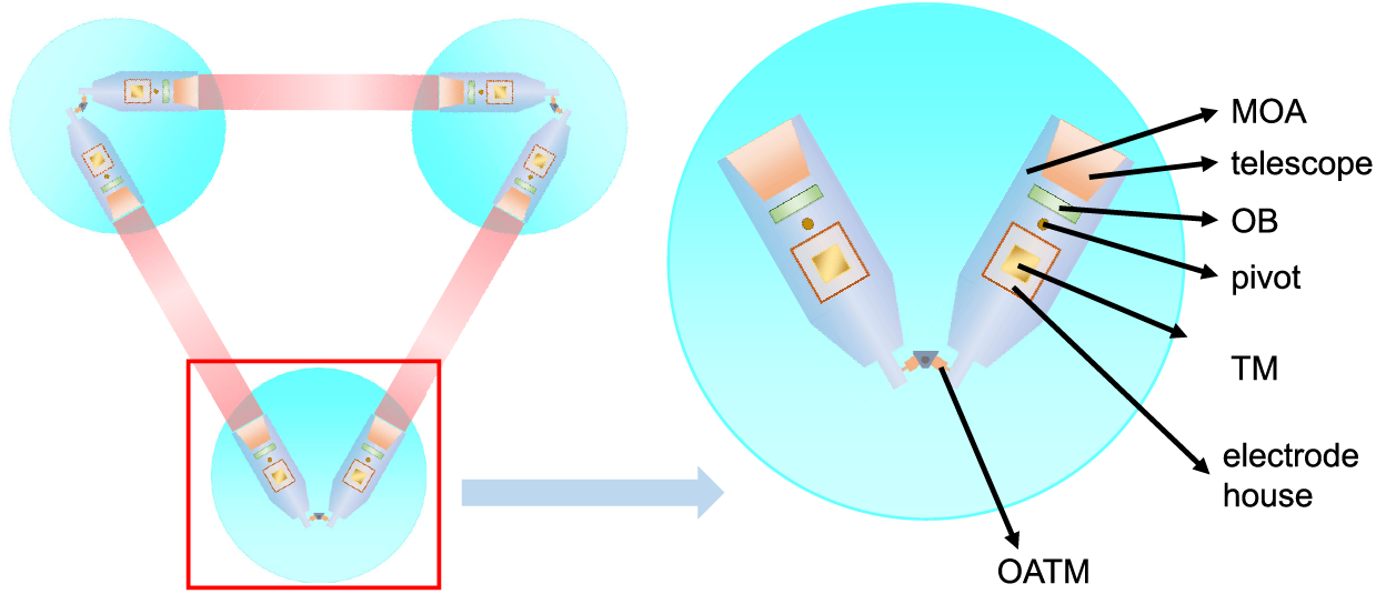
Figure 1: Gravitational wave spacecraft

In these space-based gravitational wave detection missions, the laser acquisition should be achieved prior to scientific measurement. Various acquisition schemes for different conditions are proposed [9,10]. On-ground demonstration of one laser-link construction has also been performed at [5,11,12]. Laser acquisition of formations containing three spacecraft is more complex. Laser acquisition schemes dedicated to three spacecraft have also been studied [13,14]. In the aspect of spacecraft dynamics modeling and control, a linear system dynamics model with 19 degrees of freedom (DOFs) has been presented at [15,16]. A detailed nonlinear dynamics model with 20 DOFs has been derived by Simone Vidano and the frequency response relationships between the different DOFs were also demonstrated [17].

The optical axis is defined by the optical bench (OB), which is fixed with respect to the OB without considering point-ahead angle mechanism and deformation. Thus there are 2 optical axes on a spacecraft. In the laser acquisition (Fig. 2), first the spacecraft A keeps pointing the reference direction. As the same time, spacecraft B controls the optical axis to continuously rotate for scanning. At the moment when the laser from spacecraft B covers spacecraft A, a signal is obtained on the Charge Coupled Device (CCD) of spacecraft A, which is used to determine the direction of spacecraft B. In the second step, spacecraft A adjusts its attitude so that the optical axis of spacecraft A is aligned with the orientation of spacecraft B, thus a signal is obtained on the CCD of spacecraft B. In the third step, spacecraft B performs the same attitude adjustment so that the optical axis is stably aligned with spacecraft A. At this point, the optical axes of two spacecraft enter each other’s field of view and the laser acquisition of one link is realized. The laser acquisition should be achieved between each two spacecraft.

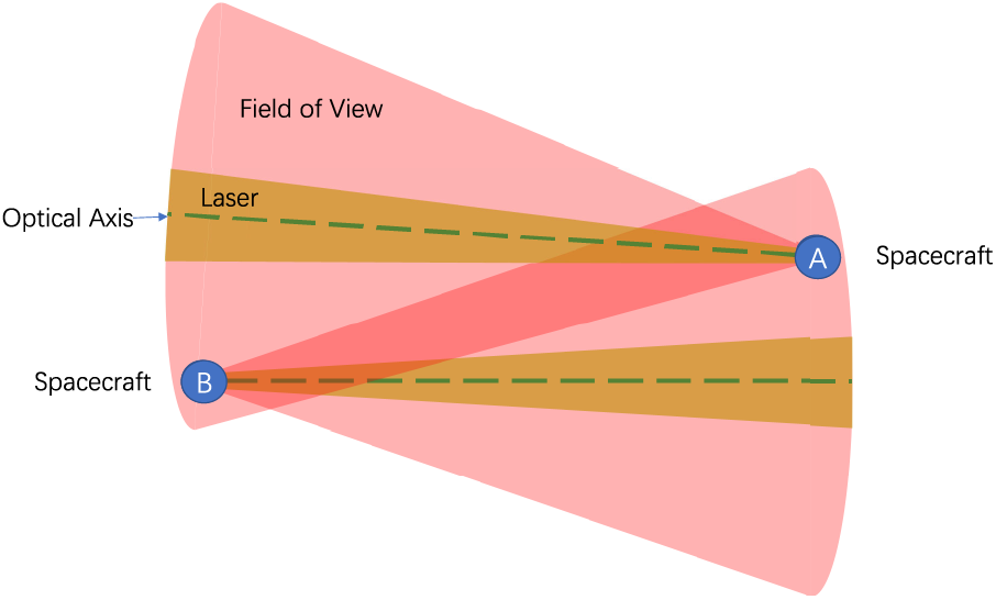
Figure 2: Laser acquisition

In Taiji program, the inter-spacecraft uncertain half-angle is 24 μ rad during the scanning phase, and the laser divergence half-angle is 1.7 μ rad. In the currently equipped attitude sensors on the gravitational wave spacecraft, the only available sensor before receiving laser from the opposite spacecraft is the star tracker sensor (STR).The accuracy of STR is 5 μ rad, which does not meet the control requirement of 1 μ rad. Therefore, during the scanning phase, considering the worst-case scenario involves insufficient accuracy in the feedback signals.

More researches are required to upgrade from the single laser-link to multi laser-links. Decoupling algorithms are necessary here. Due to complex spacecraft dynamics, each actuator leads to the motion of multiple degrees of freedom. Therefore, a decoupling module should be included in the control system to realize single-DOF motion by converting the motion demand of a single DOF into control signals to multiple actuators. In previous work, the 19 DOFs were assigned to three control loops as follows: drag-free control, spacecraft attitude control, and electrostatic suspension control. Each control loop contained an equal number of DOFs and driving forces (torques) [15]. For each control loop, decoupling could only happen within the current loop, having nothing to do with the other two loops.

The decoupling algorithm designed in this paper further addresses two problems. One is the degree of freedom problem. During the laser acquisition, the optical axes of two OBs on a spacecraft need to be controlled continuously and independently. 4 DOFs are needed for the two optical axes, while there are 3 DOFs in the spacecraft attitude control loop. Therefore, the spacecraft attitude control cannot achieve independent control of the optical axes. In previous work, the control and decoupling of the optical axis were only considered for the spacecraft’s attitude. Therefore, the earlier decoupling algorithms did not meet the requirements of degrees of freedom. Considering the entire MOA can be rotated by the OATM, the DOFs of the optical axis motion can be increased. Therefore the rotational torque of the spacecraft and the driving torque of OATM should be used to achieve the optical axis control.

The second is the motion coupling problem. Coupling causes noise transfer between different DOFs, so decoupling should minimize coupling between different DOFs. When a OATM operates, a torque is applied to the target MOA and a reaction torque is applied to the rest of the spacecraft. This can cause coupling problems between the optical axis motions. The rotational torque of the spacecraft can be used to offset the reaction torque of the OATM to reduce the coupling. Thus, the rotational torque of the spacecraft and the driving torque of the OATM should be put into a control loop for decoupling.

In response to the requirements of one spacecraft with two laser links in gravitational wave detection, this paper proposes the upgraded decoupling algorithms. The three control loops of the spacecraft control system are reassigned. Unlike previous work, optical axis control and decoupling in this study are not only focused on the spacecraft’s attitude but also involve Optical Assembly Tracking Mechanism. The driving torque of the OATM and the rotational torque of the spacecraft are assigned to the optical axis control loop, to achieve independent control of optical axes. The transfer function compensation method is proposed to reduce the coupling by analyzing the linear dynamics model of the spacecraft. The decoupling effect is verified by the open-loop frequency response of the decoupled system. The open-loop performance also affects the subsequent closed-loop control performance.

In Section 2, the overall control system framework is presented, the driving forces (torques) and DOFs are reassigned to the three control loops. In Section 3, the transfer function of the decoupler is given by analyzing the dynamics model and different decoupling algorithms are designed. In Section 4, the frequency response analysis of the open-loop system is performed to evaluate the effectiveness of the decoupling algorithms.

2  Control Systems and Control Loops

The spacecraft’s control system is shown in the red dashed box in Fig. 3. The controller contains 20 Single-Input Single-Output (SISO) control units. Each element of the control vector η output by the controller represents a control signal for one DOF. The decoupler converts the control vector η into the control signal for each driver. The drivers output driving forces and torques u. DOFs x1 are measured by sensors mounted on the spacecraft (with redundancy). The more accurate estimate of each DOF is given by the state observer through fusing u and the measured values [16].

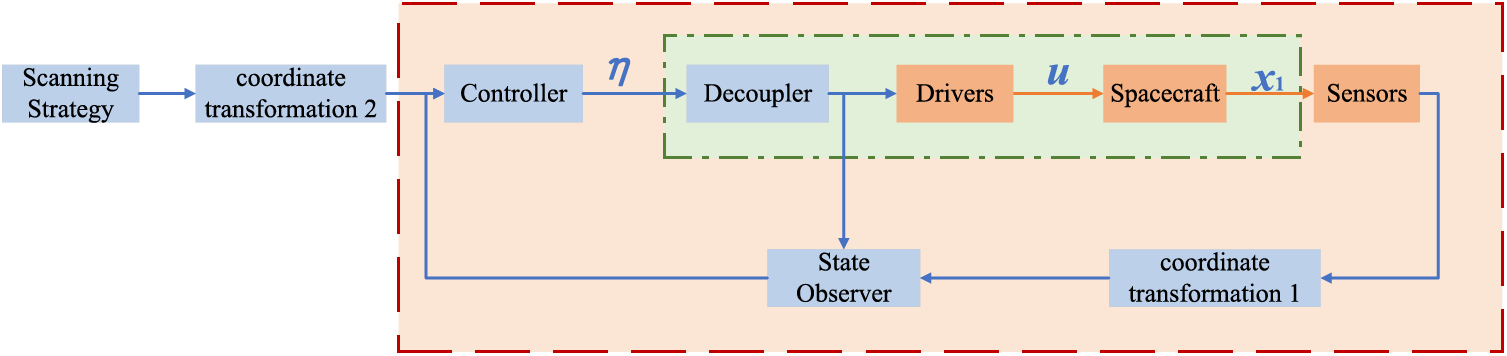
Figure 3: Gravitational wave spacecraft control system structure

CCD and Quadrant photodiodes (differential wavefront sensing, effective after attitude adjustment) [18–20] are used to measure the position of the target spacecraft. The description of the OB attitude need to be converted into the description of the spacecraft attitude and MOA turning angle relative to the nominal angle by the coordinate transformation (the relevant method can be found in the literature [21,22]). This is the coordinate transformation 1 after the sensor in the control system of Fig. 3. Scanning is required during laser acquisition, and the scanning strategy provides the maneuvering signal for the optical axis [23] that needs to be converted to control signals for spacecraft rotation and MOA rotation. Then they are provided to the controller. This is coordinate transformation 2 after the scanning strategy.

During the laser acquisition, if one spacecraft has already established one laser link, the established laser link is kept while establishing another laser link, and then the other optical axis is controlled for scanning or alignment. The optical axes of both OBs of one spacecraft needed to be controlled independently (4 DOFs are required). The DOFs controlled by the optical axis control loop should include 3 DOFs of the spacecraft attitude and the rotation angle of the MOA. The driving torque of the optical axis control loop should include the spacecraft rotational torque and the driving torque of the OATM. The spacecraft rotational torque and the driving torque of the OATM need to be collaboratively controlled and jointly decoupled in the optical axis control loop. Therefore, the spacecraft control system is divided into three control loops: drag-free control, optical axis control and electrostatic suspension control. The DOFs and driving forces and torques in each control loop are listed in the Table 1.

3  Decoupling Algorithm Design

3.1 Dynamics Model

In this paper, we use MATLAB Simscape to build the nonlinear dynamics model of the spacecraft in Fig. 3, and the schematic diagram of the simscape model is as follows Fig. 4.

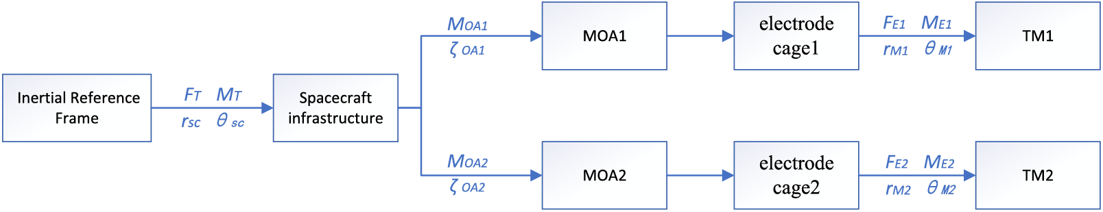
Figure 4: The schematic diagram of the gravitational wave spacecraft dynamics model

For the dynamics model, the input vector u is the driving force and torque (described in Table 2), and the output vectors x1 are the positions and angles of the DOFs (described in Table 3).

u=[FT,MT,MOA1,MOA2,FE1,ME1,FE2,ME2]T(1)

x1=[rSC,θSC,ζOA1,ζOA2,rM1,θM1,rM2,θM2]T(2)

Therefore, a 20 * 20 Multiple-In Multiple-Out (MIMO) system is used in this paper. After the start of the drag-free control, only 3 of the 6 DOFs translational forces on the TM will be used, and the other 3 directions will be tracked by driving the spacecraft translations without applying electrostatic forces.

3.2 Transfer Function of Decoupler

After obtaining the the spacecraft nonlinear dynamics model, the state space equation can be obtained by the linearization at the working point, and the initial working point is selected as

x1=0x˙1=0

The state space equation is obtained as

x˙=Ax+Bu

y=Cx+Du

D=0

where x is the 40-dimensional state variable, including state vector x1 and its first-order derivative x2 and therefore x can be decomposed,

x=[x1x2]

Decomposing A and B similarly, the state space equation is written as

[x˙1x2˙]=[0IA1A2][x1x2]+[B1B2][u]

B1=0

It can be written as two equations,

x1˙=x2(3)

x2˙=A1x1+A2x2+B2u(4)

Substituting Eq. (3) into Eq. (4),

x1¨=A1x1+A2x1˙+B2u

Perform Laplace transform,

X1s2=A1X1+A2X1s+B2U

The transfer function of driving forces (torques) to DOFs is

G=X1U=B2(Is2−A2s−A1)

For the decoupler, the input is the control signal of DOFs η, and the output is the control signal for the driving force (torque) u. The corresponding Laplace transforms are noted as H, U, respectively. The transfer function of an ideal decoupler is

D2=UH=B2−1(I−A21s−A11s2)(5)

The transfer function of the decoupler and spacecraft dynamics model is

X1H=1s2(6)

It can be seen that the transfer function compensation is performed when use Eq. (5) to decouple, in this way the decoupler and the spacecraft dynamics model present the dynamics of the second-order integral within a certain range.

In the previous decoupling design, there are only scale factors in the transfer function of the decoupler,

D1=B2−1(7)

The above D1, D2 are used to decouple the entire spacecraft, which are 20 * 20 matrixes of transfer functions. The 20 * 20 transfer functions are not all necessary in the actual control system. In other words, not all 20 driving forces (torques) but only the driving forces assigned to the corresponding control loop are used to control one DOF.

3.3 Decoupling Algorithm

Each decoupling algorithm can be divided into two parts. One is the transfer function, which can be D1 or D2. The other is the assignment of the DOFs and the driving forces (torques) which can be represented in Fig. 5. Each cell represents the transfer function from the DOFs to the driving force (D1 or D2). Red represents drag-free control, yellow represents optical axis control, and green represents electrostatic suspension control. Blue represents the transfer function that is not used.

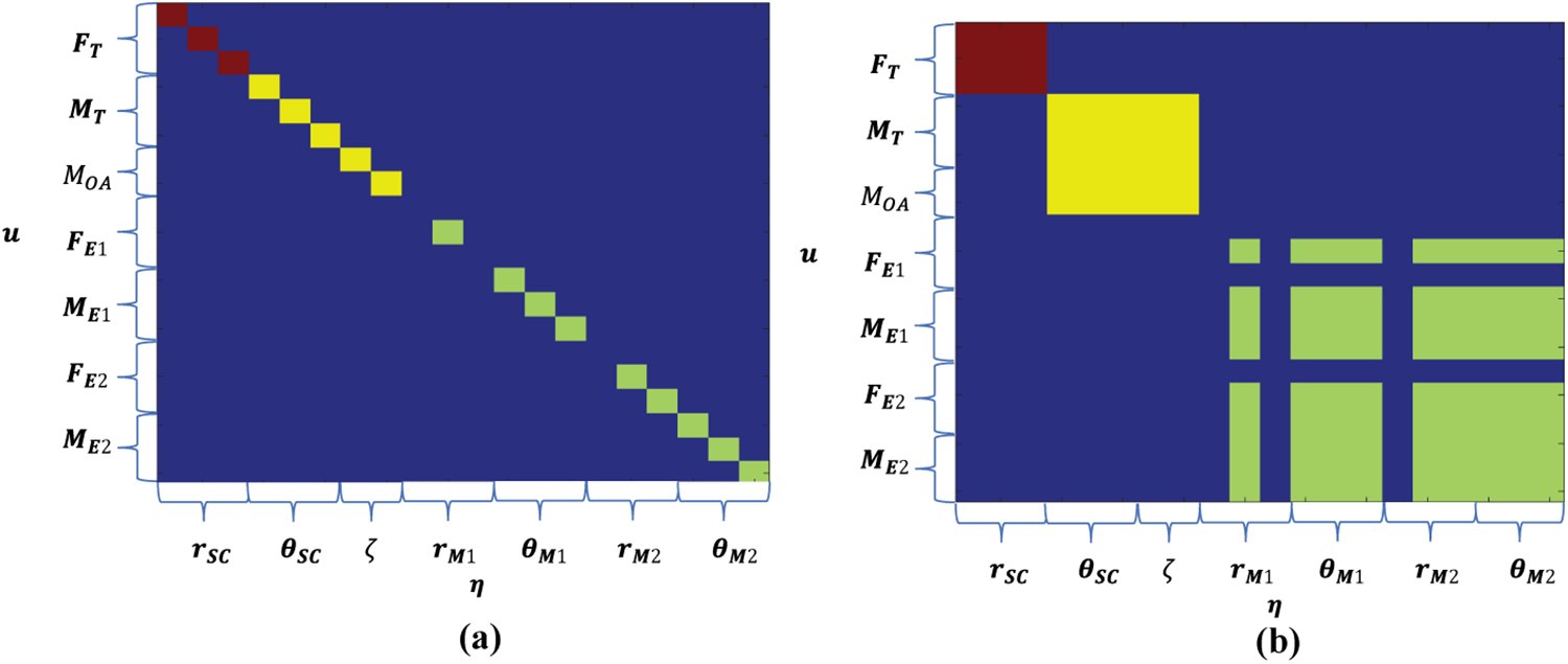
Figure 5: Input control vector of the decoupler η and output driving force u distribution relationship

Decoupling algorithm I: Only one driving force (torque) will be used to control one DOF. The input (DOF to be controlled) and output (driving force and torque) distribution of the decoupler can be represented in (a) in Fig. 5, with the transfer function using D1. There is only one scale factor between the control signal and the corresponding driving force for each DOF.

Decoupling algorithm II: Decoupling is performed within each control loop so that the driving forces (torques) within corresponding control loop are used to control one DOF. The input and output distribution of the decoupler is represented in (a) in Fig. 5. The missing rows and columns in the electrostatic suspension control are the 3 DOFs used for drag-free control. The transfer function is D1.

Decoupling algorithm III: Decoupling is performed within each control loop (Fig. 5). The transfer function is D2 to perform transfer function compensation.

4  Decoupling Evaluation

The decoupling effect can be evaluated by analyzing the open-loop frequency response of the decoupler and the spacecraft dynamics model represented in Fig. 4. It corresponds to Fig. 3 to the part inside the green dotted box, ignoring the characteristics of the drivers. The effect of decoupling is evaluated by the frequency response of the input vector η to the output vector x1 (Fig. 6). The control frequency of the drag-free control and optical axis control is less than 10 Hz due to the limitation the micro-thruster’s response time and the sensor’s sampling speed [15]. Therefore, the main frequency band during laser acquisition is 1–10 Hz. Frequency points at 1, 10, and 0.01 Hz are selected for test. 1 Hz is closest to the control system’s frequency, 10 Hz represents the upper limit of the control system’s frequency, and 0.01 Hz reflects low-frequency drift noise.

Figure 6: Open-loop system used for frequency response simulation

Fig. 7 is the frequency response at 1 Hz of the input vector η to the output vector x1 for different decoupling algorithms in decibels (dB) (20 dB represents a tenfold difference). Frequency responses that are 80 dB below the maximum frequency response are always indicated in blue. The green color is about 10−1 of the major frequency response, blue is about 10−2 of the major frequency response and yellow is the frequency response that is important or causes severe motion coupling. The cells on the diagonal represent the response of the target DOFs η in consistent with the actual DOFs x1. The two yellow boxed cells in each figure represent TM translational motion relative to the electrode cage rM caused by spacecraft translational motion rSC that is required to perform drag-free control. The other responses between different DOFs cause noise coupling and need be minimized. The red box is the optical axis control, which is our main concern.

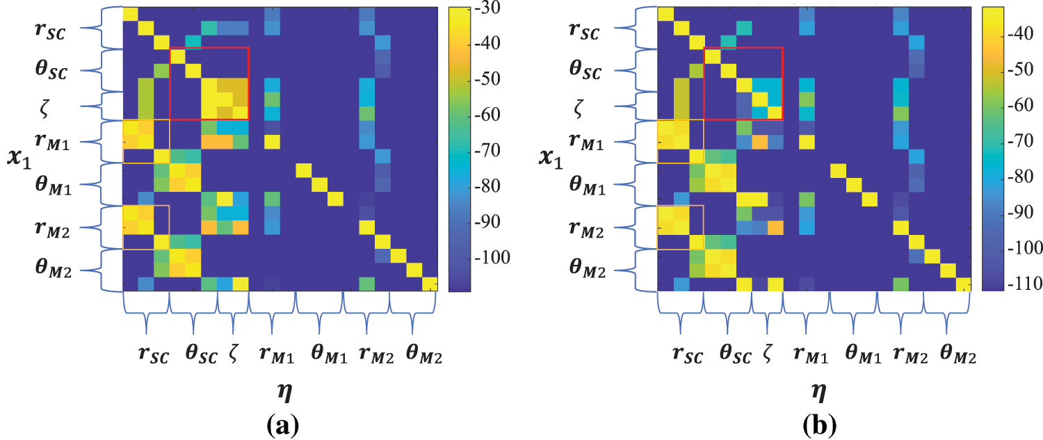
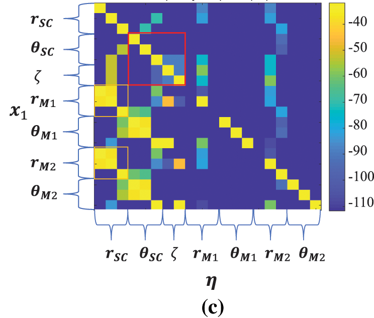
Figure 7: The frequency response at 1 Hz of the input vector η to the output vector x1 (a) Decoupling algorithm I (b) Decoupling algorithm II (c) Decoupling algorithm III

Table 4 records the maximum frequency response between different DOFs in optical axis control, i.e., unwanted motion coupling, and a smaller frequency response means a better decoupling effect.

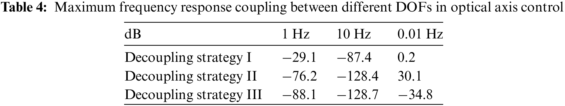
The frequency response at 1 Hz is analyzed first (Fig. 7). It can be seen that the decoupling algorithms II and III significantly reduce the coupling in the optical axis control. The decoupling algorithm II effectively reduces the coupling by offsetting the reaction torque of the OATM. Decoupling algorithm III also reduces the coupling in the optical axis control. For most DOFs, the dynamics of the system are second-order integrated without stiffness and damping, but for OATM, stiffness and damping exist. The collaborative motion produces errors due to different dynamics properties. The transfer functions compensation is used to modify the dynamics of OATM to a second-order integral model in decoupling algorithm III, thus reducing the motion coupling. For the coupling of other DOFs, the algorithms II and III are basically the same as the decoupling algorithm I.

At the higher frequency point of 10 Hz (Fig. 8), the decoupling algorithms II and III still effectively reduce coupling. However, the difference between the decoupling algorithms II and III has diminished. At the lower frequency of 0.01 Hz, the decoupling algorithm II shows a deterioration compared to the decoupling algorithm I. The decoupling algorithm III still effectively reduces coupling. The main reason is that, in the low-frequency range, the frequency response of DOFs with second-order integrator characteristics (without damping and stiffness) far exceeds that of DOFs with damping and stiffness. Decoupling algorithm III addresses this issue through transfer function compensation. However, in practical usage, the performance may not be as ideal due to the limitation imposed by actuator resolution.

Figure 8: The frequency response of the input vector η to the output vector x1. The columns from left to right are the decoupling algorithms I, II, III.The frequency points in Figs. a, b, and c are at 10 Hz. The frequency points in Figs. d, e, and f are at 0.01 Hz

In addition, the transfer function compensation method is also meaningful in cases where the output of the driver is the angle of rotation rather than the torque. This method can also be used to solve the problem of different units of input variables.

5  Conclusion

During the laser acquisition, the optical axes on a spacecraft need to be controlled independently. This imposes different decoupling requirements on the control system. The decoupling algorithm is divided into two parts, control loop assignment and transfer function design. In order to achieve independent control of the optical axes, the DOFs and the driving forces are reassigned to the three control loop. The sufficient freedom of optical axis motion is achieved by introducing the driving torque of OATM. The coupling problem due to reaction torque is reduced by decoupling in one control loop. The transfer function compensation method is used to reduce the coupling due to the different dynamics of the drivers. The open-loop simulation demonstrates that the decoupling algorithm significantly reduces the coupling of the optical axis. The decoupling algorithm addressed the motion coupling issue from a single laser link to a dual laser link on one spacecraft.

Acknowledgement: The authors are thankful to the anonymous reviewers for improving this article.

Funding Statement: This work was supported by the National Key Research and Development Program of China (2022YFC2203700).

Author Contributions: The authors confirm contribution to the paper as follows: analysis and discussion: Xue Wang, Xingguang Qian, Jinke Yang; study conception and design: Xue Wang; draft manuscript preparation: Xue Wang, Yikun Wang, Weizhou Zhu, Zhao Cui; management and coordination: Jianjun Jia. All authors reviewed the results and approved the final version of the manuscript.

Availability of Data and Materials: The data and related programs are available from the first and corresponding authors upon reasonable request.

Conflicts of Interest: The authors declare that they have no conflicts of interest to report regarding the present study.

References

1. Amaro-Seoane, P., Audley, H., Babak, S., Baker, J. et al. (2017). Laser interferometer space antenna. A proposal in response to the ESA call for L3 mission concepts. https://arxiv.org/abs/1702.00786 [Google Scholar]

2. Luo, Z., Wang, Y., Wu, Y., Hu, W., Jin, G. (2020). The Taiji program: A concise overview. Progress of Theoretical and Experimental Physics, 2021(5), 05A108. https://doi.org/10.1093/ptep/ptaa083 [Google Scholar] [CrossRef]

3. Mei, J., Bai, Y. Z., Bao, J., Barausse, E., Lin, C. et al. (2020). The TianQin project: Current progress on science and technology. Progress of Theoretical and Experimental Physics, 2021(5), 05A107. https://doi.org/10.1093/ptep/ptaa114 [Google Scholar] [CrossRef]

4. Qiao, D., Zhou, X., Li, X. (2023). Feasible domain analysis of heliocentric gravitational-wave detection configuration using semi-analytical uncertainty propagation. Advances in Space Research, 72(10), 4115–4131. https://www.sciencedirect.com/science/article/pii/S0273117723006300 [Google Scholar]

5. Gao, R., Wang, Y., Cui, Z., Liu, H., Liu, A. et al. (2023). On-ground demonstration of laser-link construction for space-based detection of gravitational waves. Optics and Lasers in Engineering, 160, 107287. [Google Scholar]

6. Zhu, W., Guo, Y., Jin, Q., Wang, X., Qian, X. et al. (2023). Measurement of the optical path difference caused by steering mirror using an equal-arm heterodyne interferometer. Photonics, 10(12), 1365. https://www.mdpi.com/2304-6732/10/12/1365 [Google Scholar]

7. Vidano, S., Novara, C., Pagone, M., Grzymisch, J. (2022). The LISA DFACS: Model Predictive Control design for the test mass release phase. Acta Astronautica, 193, 731–743. https://www.sciencedirect.com/science/article/pii/S0094576521007025 [Google Scholar]

8. Ira Thorpe, J., Stebbins, R. (2010). Preliminary investigations of an optical assembly tracking mechansim for LISA. 38th COSPAR Scientific Assembly, vol. 38. Bremen, Germany. [Google Scholar]

9. Wuchenich, D. M. R., Mahrdt, C., Sheard, B. S., Francis, S. P., Spero, R. E. et al. (2014). Laser link acquisition demonstration for the grace follow-on mission. Optics Express, 22(9), 11351–11366. [Google Scholar] [PubMed]

10. Gao, R. H., Liu, H. S., Luo, Z. R., Jin, G. (2019). Introduction of laser pointing scheme in the taiji program. Chinese Optics, 12(3), 425–431. [Google Scholar]

11. Sanjuan, J., Gohlke, M., Rasch, S., Abich, K., Görth, A. et al. (2015). Interspacecraft link simulator for the laser ranging interferometer onboard grace follow-on. Applied Optics, 54(22), 6682–6689. [Google Scholar] [PubMed]

12. Wang, Y. K., Meng, L. Q., Xu, X. S., Niu, Y., Qi, K. Q. et al. (2021). Research on semi-physical simulation testing of inter-satellite laser interference in the China Taiji space gravitational wave detection program. Applied Sciences, 11(17), 7872. [Google Scholar]

13. Maghami, P. G., Hyde, T. T., Kim, J. (2005). An acquisition control for the laser interferometer space antenna. Classical and Quantum Gravity, 22(10), S421. [Google Scholar]

14. Cirillo, F., Gath, P. F. (2009). Control system design for the constellation acquisition phase of the LISA mission. Journal of Physics: Conference Series, 154(1), 012014. [Google Scholar]

15. Gath, P., Schulte, H. R., Weise, D., Johann, U. (2007). Drag free and attitude control system design for the LISA science mode. AIAA Guidance, Navigation and Control Conference and Exhibit, Hilton Head, South Carolina, USA. https://doi.org/10.2514/6.2007-6731 [Google Scholar] [CrossRef]

16. Cirillo, F. (2007). Controller design for the acquisition phase of the LISA mission using a Kalman filter (Ph.D. Thesis). University of Pisa, Italy. [Google Scholar]

17. Vidano, S., Novara, C., Colangelo, L., Grzymisch, J. (2020). The LISA DFACS: A nonlinear model for the spacecraft dynamics. Aerospace Science and Technology, 107, 106313. [Google Scholar]

18. Wanner, G., Heinzel, G., Kochkina, E., Mahrdt, C., Sheard, B. S. et al. (2012). Methods for simulating the readout of lengths and angles in laser interferometers with gaussian beams. Optics Communications, 285(24), 4831–4839. [Google Scholar]

19. Hechenblaikner, G. (2010). Measurement of the absolute wavefront curvature radius in a heterodyne interferometer. Journal of the Optical Society of America A, 27(9), 2078–2083. [Google Scholar]

20. Luo, Z., Gao, R., Liu, H., Jin, G. (2020). Linearity performance analysis of the differential wavefront sensing for the taiji programme. Journal of Modern Optics, 67, 383–393. [Google Scholar]

21. Houba, N., Delchambre, S., Ziegler, T., Hechenblaikner, G., Fichter, W. (2022). Lisa spacecraft maneuver design to estimate tilt-to-length noise during gravitational wave events. Physical Review D, 106, 022004. [Google Scholar]

22. Houba, N., Delchambre, S., Ziegler, T., Fichter, W. (2022). Optimal estimation of tilt-to-length noise for spaceborne gravitational-wave observatories. Journal of Guidance, Control, and Dynamics, 45(6), 1078–1092. https://doi.org/10.2514/1.G006064 [Google Scholar] [CrossRef]

23. Ales, F., Gath, P., Johann, U., Braxmaier, C. (2015). Line of sight alignment algorithms for future gravity missions. AIAA Guidance, Navigation, and Control Conference, Kissimmee, Florida, USA. https://doi.org/10.2514/6.2015-0094 [Google Scholar] [CrossRef]