Fractional Discrete-Time Analysis of an Emotional Model Built on a Chaotic Map through the Set of Equilibrium and Fixed Points

1  Introduction

An evolution function, a chaotic map, refers to a map exhibiting some kinds of chaotic and transient behaviors, and in that regard, it is possible to parameterize the maps by a discrete-time or a continuous-time parameter. While discrete maps typically take the form of iterated functions, chaotic maps, often generating fractals, usually arise in the study of dynamical systems with ever-evolving properties. Considering that a fractal can be constructed by an iterative procedure, some fractals are to be studied as sets instead of the map generating them due to the presence of having different iterative procedures to generate the very same fractal. Regarded as one of the most rooted literatures of the world, the Persian literature includes the well-known deeply tragic and epic love story of Layla and Majnun. Different poems, plays, and operas have attempted to interpret the story in various artistic ways. Although it is difficult to develop a mathematical model particularly for this story, it is possible to probe and investigate ways to use mathematical ideas and methods to express various features of the story. One related strategy is to simulate the evolution of the love between Layla and Majnun’s intensity or strength over time. This intensity can be expressed mathematically using a function that takes into account factors including how long it has been since they first met, current relationship obstacles, and each person’s emotional condition. It is possible for this function to consider complex emotions like happiness, yearning, pain and hopelessness, with the ultimate core message of idealization of love and underlying hint of undying love.

Multiple interacting factors of systems with cyclic patterns have to do with many branches of possible states and high-dimensional manifolds in nonlinear dynamics, which requires one to take into account the historical and evolutionary path that has been through many different critical points in diverse phenomena [1]. The sensitive dependence on initial conditions results in a degree of unpredictability, which is common in romantic relationships. Complex variables are said to have both magnitude and phase, so they can represent love better and more complex emotions like the coexisting love and hate. The model shows the treating of the feelings as a two-dimensional vector rather than a scalar, which is a step closer to reality [2].

The model has discussed the romantic connections between Layla and Majnun. The nonlinear system with two complex variables is described in its most basic form [2–4]

dΩdτ=ρ1Ω(τ)+Λ2(τ)+σ1dΛdτ=ρ2Λ(τ)+Ω2(τ)+σ2,(1)

where Ω and Λ indicate the feeling of them; while ρ1,ρ2 and σ1,σ2 are the coefficients of the system satisfying ρ1<0,ρ2<0,σ1>0 (each has sympathy to Majnun) and σ2<0. Consider the Caputo fractional operator (1) (see [5] for recent effort) is defined as a complex system (four-dimensional real system of fractional differential equations) by numerous investigators. The authors in [6] presented the analytic univalent solution of a complex variable in the open unit disk

dΩdτ=ρ1Ω(τ)+Λ2(τ)+1dΛdτ=ρ2Λ(τ)+Ω2(τ)+1,(2)

where Ω and Λ are analytic functions in the open unit disk.

The recent investigation aims to formulate System (1) in terms of fractional discrete system. As a consequence, the system is analyzed to check different aspects of the stability, stabilization and controlling. Methods are provided in Section 2, while stability and fractional difference systems are presented in Section 3. Stabilizing is checked in Section 4 and the conclusion along with future directions are provided.

2  Fractional Calculus Techniques and Concepts

A branch of mathematics known as discrete fractional calculus applies the ideas of classical calculus to discrete or non-continuous contexts. Traditional calculus works with continuous functions and derivatives, but information and procedures are frequently fundamentally discontinuous in real-world situations. The goal of discrete fractional calculus is to apply fundamental calculus ideas to such discrete circumstances. Since limits are used to determine derivatives and integrals in classical calculus, they might not be directly applicable in discrete cases (for application, see [7–9]). Discrete fractional calculus uses methods from fractional calculus, which deals with derivatives and integrals of non-integer order, to describe similar procedures for discrete functions (see [10]). As the traditional concepts of derivatives and integrals are founded on the limit concept, which needs continuity, discrete fractional calculus presents a number of difficulties. For real-world issues, especially those involving discrete data, complex behavior, and non-integer order systems, the Fractional Discrete System provides a number of benefits. It is an effective tool for real-time applications in control systems, signal processing, and system modeling because to its computational efficiency, modeling versatility, handling of anomalous diffusion, and simplicity of implementation. These benefits establish the fractional discrete system as a very successful method for resolving a variety of scientific, engineering, and industrial issues [11,12].

This section of the study is concerned with the concepts and notations regarding the related fractional calculus techniques.

Definition 1. It is supplied by the arrangement that the Riemann-Liouville fractional integral, as follows:

Υaγf(τ)=1Γ(γ)∫aτ(τ−ς)γ−1f(ς)dς.

Note that, when f(τ)=1, we have

Υaγf(τ)=(τ−a)γΓ(γ),γ∈(0,1].

As a special case, when a=0, we have

Υγf(τ)=1Γ(γ)∫0τ(τ−ς)γ−1f(ς)dς.

The Caputo operator is considered, as follows:

ΔCΔγf(τ)={Υn−γf(n)(τ)=1Γ(n−γ)∫0τf(n)(ς)(τ−ς)γ−n+1dς,(n−1)<γ<ndndτnf(τ),n=γ.(3)

Definition 2. According to Caputo calculus, the fractional difference operator is characterized in the following way:

ΔCΔℵγf(τ)=Δℵ−(n−γ)Δnf(τ)=1Γ(n−γ)∑ς=ℵτ−(n−γ)(τ−ς−1)n−γ−1Δnf(ς),(4)

where f:Nℵ:={ℵ,ℵ+1,...}→R,n=1+⌈γ⌉, γ∉N where τ∈Nℵ+n−γ. Furthermore, the term τ(γ) is defined, as follows:

τ(γ)=Γ(τ+1)Γ(τ+1−γ),γ>0.

The appropriate discrete integral equation can be created via the following expression:

f(τ)=f0(τ)+1Γ(γ)∑ς=ℵ+n−γτ−γ(τ−ς−1)γ−1f(γ+ς−1).(5)

Comparable to conventional integer-order discrete systems, fractional discrete systems, sometimes referred to as fractional-order discrete systems, have a number of advantages. The following items can be pointed as some benefits of fractional discrete systems as proposed in the recent study:

•   Versatility: The concept versatility has been enhanced owing to fractional discrete systems, which make complicated processes’ modeling and control with more adaptable. They provide system dynamics descriptions more degrees of freedom by incorporating fractional-order operators. This adaptability enables more accurate representation of complex everyday events that integer-order models are unable to fully capture. It is significant to note that due to the non-local and memory-dependent character of how they operate, the study and development of fractional LMMs may be more difficult than those of integer-order systems. As a consequence, in order to utilize the adaptability of such systems for varied applications, a thorough understanding of fractional calculus, system dynamics and numerical approaches become necessary to be addressed and employed.

•   Performance improvement: By permitting more precise control, fractional discrete systems can improve system efficacy and enhanced robustness. The capacity to fine-tune system parameters owing to fractional-order dynamics results in increased stability, quicker reaction times, overshoot and better tracking of intended trajectories. Consequently, applications like control systems, signal processing and optimization can all benefit greatly from this. Compared to integer-order systems, LMMs may exhibit more complicated stability properties. To make sure the system is stable for a range of parameter values, it may become necessary to perform a stability analysis.

•   Better memory simulation: Fractional discrete systems are excellent at capturing memory effects in dynamical systems, allowing for better memory simulation. The fractional-order operators enable for a more accurate depiction of memory-based processes by taking into consideration long-term dependencies and non-local memory properties. The modeling of systems with long-term dependencies, such as time series analysis, image processing and management of intricate physical systems, benefits particularly from this property. LMMs better capture memory effects by extending the idea of discrete time-stepping to fractional orders.

•   Numerous applications: Numerous disciplines, including control engineering, signal processing, economics, biology, physics, and many more, use fractional discrete systems which are proven to be useful tools for modeling and evaluating real-world phenomena due to the fact that because they can represent complicated dynamics and memory effects, which can enable greater comprehension and better system design across a variety of fields. LMMs can be suggested for relevant purposes, for example, to analyze the signal, wave and image filtering.

Fractional Discrete-Time LMM with the Chaotic Map

The LMM chaotic map can be presented by (see Fig. 1)

{Ω(n+1)=ρ1Ω(n)+Λ2(n)+σ1Λ(n+1)=ρ2Λ(n)+Ω2(n)+σ2(6)

Figure 1: The plot of System (6) for n=1−1000, when both have equally feelings (ρ1=ρ2=−1) and for positive parameter σ1=1/300 with different negative values of σ2=−0.001,−0.101,−0.22,−0.1,−0.03,−0.003, respectively

where n∈N, and Ω and Λ are the settings of the function corresponding to the feelings of Majnun and Layla respectively. While the negative parameters are ρ1,ρ2 and σ2; and a positive parameter σ1 denoting the connection coefficients. The positive value of σ1 suggests that Majnun was seen favorably by everyone. The initials Ω2 and Λ2 denote a profound love, and evidence of goodness from one has profoundly influenced each other. The delta form of (6) can be viewed by

{ΔΩ(n)=(ρ1−1)Ω(n)+Λ2(n)+σ1ΔΛ(n)=(ρ2−1)Λ(n)+Ω2(n)+σ2.(7)

The Caputo difference given in Definition 2 can be used to implement the LMM using a definition as its starting point

{ΔℵγCΩ(τ)=(ρ1−1)Ω(τ−1+γ)+Λ2(τ−1+γ)+σ1ΔℵγCΛ(τ)=(ρ2−1)Λ(τ−1+γ)+Ω2(τ−1+γ)+σ2,(8)

where γ∈(0,1]. In virtue of the integral difference formula, System (7) can be viewed as follows (see Figs. 2 and 3 for different parameters):

{Ω(τ)=(ρ1−1)Ω(ℵ)+1Γ(γ)∑ς=ℵ+1τ−γ(τ−ς−1)γ−1Λ2(τ−1+γ)+σ1Λ(τ)=(ρ2−1)Λ(ℵ)+1Γ(γ)∑ς=ℵ+1τ−γ(τ−ς−1)γ−1Ω2(τ−1+γ)+σ2,(9)

where

(τ−ς−1)γ−1Γ(γ)=Γ(τ−ς)Γ(γ)Γ(τ−ς−γ+1)

presents the discrete kernel function. For special case, when ℵ=0, System (9) becomes

{Ω(τ)=(ρ1−1)Ω(0)+1Γ(γ)∑ς=1τ−γ(τ−ς−1)γ−1Λ2(τ−1+γ)+σ1Λ(τ)=(ρ2−1)Λ(0)+1Γ(γ)∑ς=1τ−γ(τ−ς−1)γ−1Ω2(τ−1+γ)+σ2.(10)

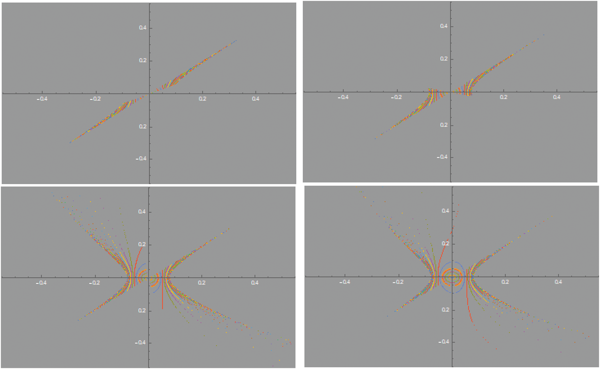
Figure 2: The plot of fractional System (10) for n=1−1000, when both have equally feelings (ρ1=ρ2=−0.001) and for positive parameter σ1=1/300 and σ2=−0.003 with different fractional values γ=0.25,0.5,0.75,0.975, respectively

Figure 3: The plot of fractional System (10) for n=1−1000, when both have equally feelings (ρ1=ρ2=−0.01) and for positive parameter σ1=1/300 and σ2=−0.003 with different fractional values γ=0.25,0.5,0.75,0.975, respectively

Remark 1. In this remark, we present alternative class of two fractal derivatives to generalize System (1). We start with the fractal-MEMS concept. Research on fractional discrete systems is a new and exciting field, particularly in fractal MEMS (Micro-Electro-Mechanical Systems). Although this discipline is still in its infancy, the combination of fractional calculus and fractal geometry in MEMS opens up a number of useful applications. Energy loss resulting from non-Newtonian damping caused by surface properties in a MEMS resonator with fractal shape can be described by fractional differential equations. In fractal MEMS resonators, fractional calculus aids in more precise damping modeling. In a MEMS gyroscope with fractal features, fractional control can improve angular velocity precision when measuring or settle oscillations. Furthermore, improved resonance matching for environmental vibrations can be achieved with a fractal piezoelectric MEMS harvester that uses fractional-order circuits. The idea is coming from the determination of limit

Λ=limε→0log⁡Σ(ε)log⁡(1/ε),

where ε indicates the size of the box, while Σ(ε) is the number of boxes that can be covered by a fractal. Introducing fractal dynamics or fractional discrete systems into an emotional movement system, like a love story can have special benefits that improve audience engagement, realism, and emotional depth. A novel approach to modeling emotional complexity, visualizing linkages, and developing deeper narrative layers is provided by the incorporation of fractal dynamics and fractional discrete systems into a love story. Storytellers may create engrossing, complex, and poignant narratives that reflect the complex and uncertain nature of relationships in the actual world by utilizing these mathematical ideas.

Remark 2. The investigation of fractal calculus, which applies conventional calculus methods to fractional and fractal geometries, gives development to the idea of the two-scale fractal derivative. When characterizing processes that display complicated, self-similar, or non-integer-dimensional behavior, which is frequently observed in a variety of domains, including physics, biology, and finance. The concept behind the two-scale fractal derivative is to take into consideration activity at two distinct scales: a coarse size, where fractal-like behavior predominates, and a fine scale, where standard differentiation is appropriate. This method results in a generalization of the derivative, where the rate of change of a function is quantified according to of its fractal character at various scales as well as its local variation.

The main formula for this type of fractal is given in [13], as follows:

Dηg(χ)=lim(g(χ+εη)−g(χ)εη).

And it is modified by the formula

D2η,η′g(χ)=lim(g(χ+εη)−g(χ)εη)+λ(g(χ+εη′)−g(χ)εη′),

where λ is a scaling factor. The value of λ is a parameter that controls the coupling between fine-scale (short-term) and coarse-scale (long-term) in a motion dynamic system, such as a love story. The degree to which long-term patterns or more profound emotional exchanges impact the system’s (the relationship’s) current state will depend on the value of λ.

Application 1. Our application is fractional digital filter design for MEMS. Similar to accelerometers, MEMS sensors frequently generate noisy data. While maintaining signal integrity, fractional-order filters are more successful in reducing noise than integer-order filters. This process can be vied as fractional difference equation for digital filters, as follows:

f[n]=∑k=0NφnΔNγCχ[n−k]+∑k=1Mϕkf[n−k],

where χ[n] indicates the input signal, f[n] is the output signal, φk and ϕk present the filter coefficients and CΔℵγ represents the represents the fractional backward difference operator. The coefficients are determined (the memory effect of the fractional filter is represented by these coefficients), as follows:

φk=Γ(1+γ)Γ(1+k)Γ(1+γ−k).

Similarly for ϕk. When γ=0.5, we have

φ0=1,φ1=−0.5,φ2=−0.125,φ3=−0.0625,φ4=−0.0391,...

For bigger k, the coefficients decay quickly but do not become small, indicating that the system retains long-term memory (see Fig. 4).

Figure 4: The plot of fractional order and integer order filter on noisy MEMS data. The Fractional-Order Filter (γ=0.5) (blue) smoothes out noise while maintaining the amplitude and form of the actual signal. The red integer-order low-pass filter minimizes noise but more significantly blurs and affects the actual signal

3  Stability and Fractional Difference Systems

The investigation of the stability of fractional-order singular systems happens to be more complex than the investigation of integer-order singular systems; and thus, it is intriguing to examine the stability of fractional-order singular systems that are significant in theory and application-related aspects. The behavior of systems that are described by fractional difference equations is examined as part of the stability analysis of fractional difference systems. The concept of discrete-time systems is made more generic by fractional difference equations by allowing for non-integer orders of difference. Numerous methods, such as frequency domain analysis and Lyapunov stability analysis, can be used to evaluate the stability of such systems.

Stability Criteria: In conjunction with the methods mentioned above, there are stability standards created especially for fractional difference systems. In order to provide the necessary and adequate requirements for stability based on the value of the coefficients of the system’s characteristic polynomial, the Routh-Hurwitz stability criterion has been extended to fractional difference equations, as an example.

It is crucial to keep in mind that stability analysis for fractional difference systems is a current area of research, and the available techniques may change based on the particulars of the system and the parameters of the fractional difference equation being researched. Therefore, for a thorough examination of the stability of a particular fractional difference system, it is advised to refer to specialized literature or contact authorities concerned with the subject-matter.

At this point, we check the global stability of the fractional LMM utilizing the information of the characteristic polynomial’s stability. A topic linked to the stability of a system given by a linear time-invariant (LTI) differential equation is the stability of the characteristic polynomial. The stability characteristics of the system are determined by the characteristic polynomial, which is generated from the differential equation’s coefficients. The characteristic polynomial is frequently connected to the transfer function’s numerator in the context of control systems. The characteristic polynomial for a continuous-time LTI system is created by setting the transfer function’s denominator to zero. Similar to this, it is created for a discrete-time LTI system by zeroing out the numeric part of the transfer function for the z-transform.

3.1 Linear System of the Fractional LMM

The subsequent concept can be presented herein.

Definition 1. Assume that Φ(χ)=Φ(χ;χ0,Φ0) is an outcome of the fractional LMM

ΔCΔγΦ(χ)=Ψ(χ,Φ),τ∈[χ0,∞)(11)

with Φ(χ) occurs via [χ0,∞) such that

(χ,Φ(χ))∈Σ:={(χ,Φ(χ)):χ∈(ς1,∞),‖Φ‖<χ0,χ>χ0}.

Then Φ is stable if for a positive number p>0, for every outcome Φ(χ)=Φ(χ;χ0,Φ0)∈Σ satisfying the inequality

‖Φ1−Φ0‖<p,p>0.

And if for available positive number q>0 satisfies 0<q≤p then

‖Φ1−Φ0‖<q⇒

‖Φ(χ;χ0,Φ0)−Φ(χ;χ0,Φ1)‖<p,χ∈[χ0,∞).

In addition, if

limχ→∞‖Φ(χ;χ0,Φ0)−Φ(χ;χ0,Φ1)‖=0

then the outcome has attained asymptotic stability.

The stability models that we have are as follows:

Theorem 1. Consider the following n-dimensional linear system

ΔγC(υ1(χ)...υn(χ))=Zn×n(χ)(υ1(χ)...υn(χ)).(12)

Then, the solutions of (12) are stable if and only if they are bounded, every possible solution to the continuous system associated with (7) is stable. In addition, the outcomes remain asymptotically stable if the characteristic polynomial of Z accepts the stability phenomenon.

Proof. Define a matrix-valued function with double variables using the fractional integral operator, as follows:

Θ(χ,χ0)=Id+ΥγZ(χ)+ΥγZ(χ)ΥγZ(x1)+...+ΥγZ(χ)ΥγZ(x1)...ΥγZ(xn−1)+...,

where Id is the identity matrix satisfying the equality

Θ(χ0,χ0)=Id.

In actuality, all (12) system solutions are bounded, which means that there is a positive integer p>0 that the system’s fundamental matrix can obtain. ‖Θ‖<p, where ‖.‖=max|.| This brings

‖υi(χ)−υi(χ0)‖<εnp,ε>0,i=1,...,n.

Consequently, we obtain

‖υi(χ;χ0,υi(χ0))−υi(χ;χ0,υi(χ1)))‖=‖Θ(χ,χ0)(υi(χ0)−υi(χ1))‖<npεnp=ε.

Define the vector V(χ)=(υ1(χ)...υn(χ)) such that V0=(υ1(χ0)...υn(χ0)). Thus, we get

‖V(χ)−V0‖≤‖Θ(χ,χ0)(V(χ)−V0)‖≤p‖V(χ)−V0‖<p(εnp+...+εnp)=ε.

As a result, System (3.1) solutions have become stable.

In contrast, according to the stability’s definition, for ε>0 there is a number ℘>0 satisfying

‖V(χ)‖<℘⇒‖Θ(χ)V(χ)‖<ε.

Especially,

‖vi(χ)‖=‖vi(χ;χ0,v0)‖<εn.

In general, for n−dimensional vector, we have

‖V(χ)‖<ε.

Hence, all the outcomes are bounded.

But the characteristic polynomial Ω admits a stability behavior, this introduces the following inequality:

‖V(χ;χ0,V0)−V(χ;χ0,V1)‖≤pexp⁡(Θ(χ−χ0)γγ)‖V1−V0‖≤pexp⁡(−ε1χγγ),0<ε1<ε=0,χ→∞.

This implies that the outcome is asymptotically stable. ▪

Corollary 1. Assume that ‖Θ‖<1 has eigenvalues that fall within the identity interval [0, 1]. Then, the outcomes related to System (12) have asymptotically stable conduct.

Proof. Let the assumptions of the statement hold. When this happens, Θ admits the invertible positive compression characteristic [14]. That is the characteristic polynomial Θn×n−1−Id in other words, it fulfills a favorable semi-definite characteristic, such that Det(Θn×n)>0 (see [15]). The characteristic polynomial Θ is therefore said to be real stable. In virtue of the Theorem 1, we have solutions that are asymptotically stable. ▪

The outcome for the non-homogeneous scenario is as follows:

Theorem 2. The solutions of

ΔγC(υ1(χ)...υn(χ))=Zn×n(χ)(υ1(χ)...υn(χ))+(ψ1(χ)...ψn(χ))(13)

are stable if and only if they are bounded and

‖Ψ‖=‖(ψ1(χ)...ψn(χ))‖<ρ,ρ∈(0,∞).

If the characteristic polynomial is stable, the outcomes also exhibit asymptotically stable conduct with

p<ϑρ,ρ>0,‖Θ‖≤p.

Proof. Let ‖Ψ(χ)‖<ρ,ϑ>0,ρ>0. Consequently, we obtain

‖V(χ)‖≤pexp⁡(pρχγγ)‖V0‖≤pexp⁡((pρ−ϑ)χγγ)‖V0‖=0,pρ−ϑ<0,τ→∞.

▪ According to Corollary 3, we obtain the subsequent outcome:

Corollary 2. Assume that ‖Θ‖<1 and all its eigenvalues are in the interval [0, 1]. Also, consider ‖ψ‖<ρ,ρ>0. Then System (13) has asymptotically stable solutions whenever

p<ϑρ,ρ>0,ϑ>0‖Θ‖≤p.

3.2 Observation for the System Stability

For the system

ΔCΔγΩ(τ)=ρ1Ω(τ)+Λ2(τ)+σ1ΔCΔγΛ(τ)=ρ2Λ(τ)+Ω2(τ)+σ2,(14)

the set of the eigenvalues is E={λ1,2:0,ρ1,ρ1<0}. We look at the roots of the distinctive polynomial to analyze a system’s stability. The system is deemed stable if all the roots have negative real parts. Any positive real portion in a root indicates instability in the system. Additionally, the system may behave oscillatorily if any root has zero real component (i.e., lies on the imaginary axis).

For the case ρ1=−1, the Routh-Hurwitz criterion and the Nyquist criterion are frequently used to assess stability for continuous-time systems based on the roots of the characteristic polynomial. While the Nyquist criterion links stability to the contour encirclements of the critical point (−1+i0) by the Nyquist plot, the Routh-Hurwitz criterion verifies the signs of the coefficients of the characteristic polynomial to determine the number of roots in the left half of the complex plane.

Moreover, the system when ρ1=ρ2=−1 is given by

ΔCΔγΩ(τ)=−Ω(τ)+Λ2(τ)+σ1ΔCΔγΛ(τ)=−Λ(τ)+Ω2(τ)+σ2,(15)

with the characterization of the polynomial being s2+s=0 satisfying the transfer function 1/(s−1) (see Figs. 5 and 6).

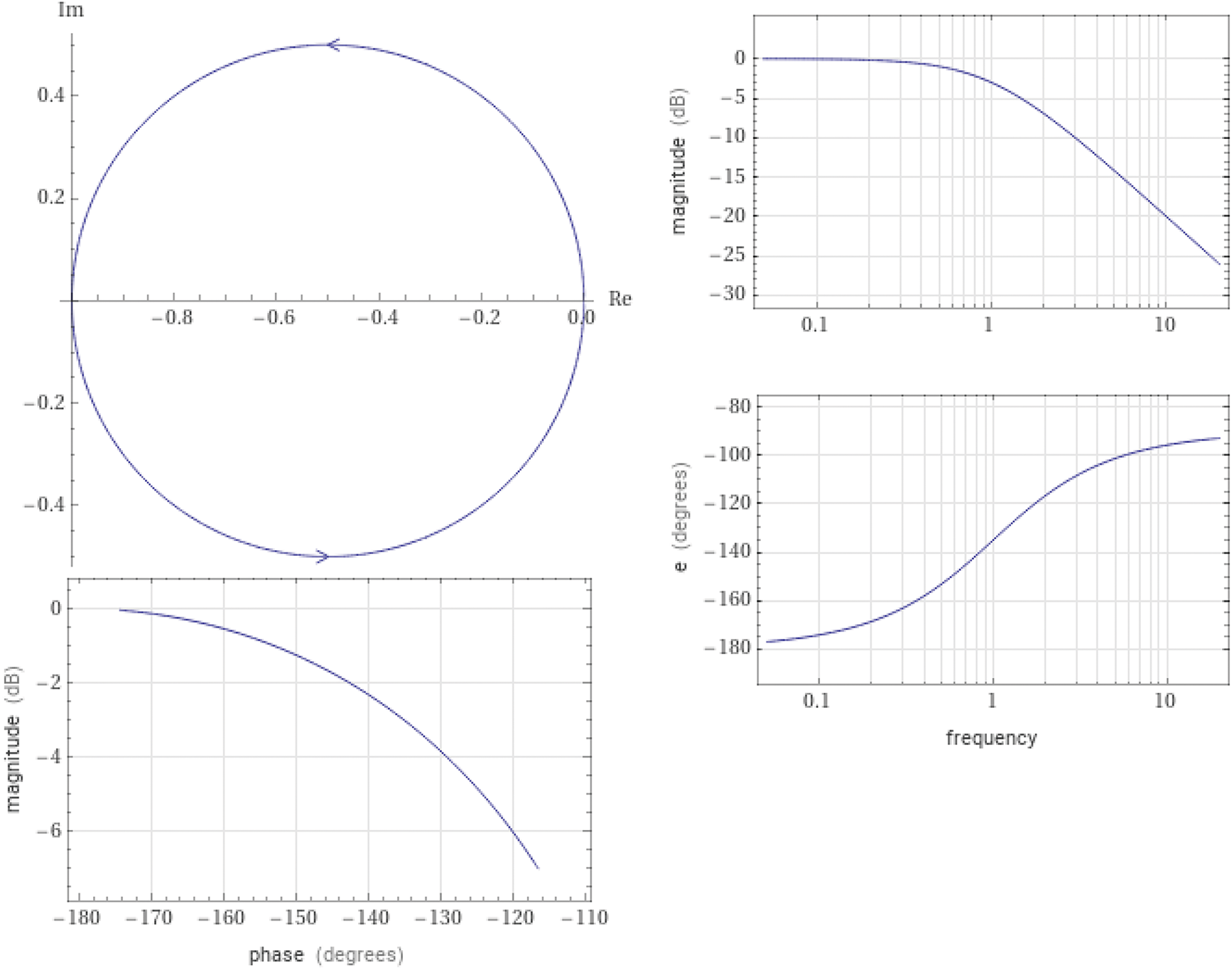
Figure 5: Nyquist plot of the transfer function 1/(s−1)

Figure 6: The directive Nyquist plot of the transfer function L(s)=1/(s−1)

In general, the system

ΔCΔγΩ(τ)=ρ1Ω(τ)+Λ2(τ)+σ1ΔCΔγΛ(τ)=ρ2Λ(τ)+Ω2(τ)+σ2,(16)

has a characteristic polynomial s2−ρ1s=0 with the transfer function L(s)=1−ρ1ss2−1. Figs. 7 and 8 show the Nyquist plot and the directive Nyquist plot, when ρ1=−0.8, respectively.

Figure 7: Nyquist plot of the transfer function 1−(−0.8)ss2−1

Figure 8: The directive Nyquist plot of the transfer function L(s)=1−(−0.8)ss2−1

3.2.1 System Analysis of Fractional LMM Over a Special Case

Assume the following system:

ΔCΔγΩ(τ)=−Ω(τ)+Λ2(τ)+1ΔCΔγΛ(τ)=−Λ(τ)+Ω2(τ)−1.(17)

The system has the following set of critical points:

Sc={(1,0),(1.2056,0.4534),(−1.103∓0.666i,−0.227±1.468i)}.

And the set of fixed points is as follows:

Sf={(0.559072,−0.34372),(2.15333,1.81842),(−1.3562∓1.52118i,−0.737353±2.06303i)}.

The Jacobian matrix is recognized by the matrix

J(Ω,Λ)=(−12Λ2Ω−1);

thus,

J(1,0)=(−102−1);

with λ1,2=−1. Hence, the system is asymptotically stable at the equilibrium point (1,0). Also, we obtain

J(1.205,0.4534)=(−10.92.4−1);

with λ1=−2.46969 and λ2=0.469694. Hence, the system is marginal stability. The system is marginally stable if its eigenvalues have both negative and zero real portions. It denotes that the system neither converges nor diverges to a steady trajectory or equilibrium point. Instead, it continues to hover along the line separating stability and instability. At this point, by using the fixed point, we get

J(0.559,−0.343)=(−1−0.6861.118−1);

Hence, we receive λ1,2=−1±0.875756i, which implies the stability of the system. Proceeding with the second fixed point

J(2.15333,1.8184)=(−13.6364.3066−1);

where λ1=−4.95712 and λ2=2.95712. Therefore, we obtain the marginal stability for the system based on the model proposed.

Remark 1. The fixed point set is essential to comprehending the stability and long-term behavior of dynamical systems. The states of the system that do not change over time are known as fixed points, or equilibrium points. In order to determine if minor perturbations surrounding fixed points will increase (signaling an unstable fixed point) or decrease (signaling a stable fixed point), stability is analyzed using fixed points. This indicates whether a system will shift from or restore to equilibrium following a perturbation.

4  Conclusion and Future Directions

When romantic relationships are modeled with differential equations, models that display complex, transient and uncertain behaviors, as encountered in real world, may remain simple algebraically. Thus, models which are capable of revealing a variety of different behaviors are required in such settings. Fractional discrete systems make complicated processes’ modeling and control with more adaptable, providing system dynamics descriptions with more degrees of freedom through the incorporation of incorporating fractional-order operators. It is this adaptability which enables more accurate representation of complex everyday events that integer-order models are unable to fully capture. In view of these points, a variety of fractional Layla and Majnun model (LMM) system types has been proposed in this investigation where we examined some of these systems’ most important and key behaviors. To these ends, we checked the fractional dynamic systems’ stability and asymptotic stability, and as a result, we provided the LMM with the specifications it needs to meet in order to obtain continuous and asymptotically steady zero resolutions. Furthermore, we also suggested a special case of these systems, besides delivering different types of stability to cover the set of equilibrium points and the set of fixed points. As a special case, when Layla and Majnun have equal feelings, we propose an analysis of the system in view of its equilibrium and fixed point sets. Therefore, it has been found and concluded that the best stability goes with equal feelings of love for Layla and Majnun (ρ1=ρ2<0). As future directions, one can use a quantum calculus or k-symbol calculus to obtain more generalization and modification for the system LMM. Based on Remark 1 and 2, System (1) can be viewed in fractal structure. Illustrates how a multi-scale method is incorporated into the two-scale fractal derivative, which generalizes the standard derivative. The values of λ and η, which regulate the scaling exponent, determine how the derivative behaves. However, there are two main limitations in the suggested system. Limitations of Simulation: The fractional order is typically a parameter that requires estimation, and choosing a suitable number can be challenging and application-specific. Physical Interpreted: In certain situations, the fractional order may not have a clear physical interpretation, which makes it more difficult to connect the system to actual operations. Understanding Complexity: Mathematical Complexity: Compared to their integer-order equivalents, fractional differences and sums are more mathematically complex, which makes analysis difficult, particularly for stability and controllable research. Non-locality: The fractional nature complicates the analytic and numerical treatment by introducing memory effects that make the system’s behavior reliant on its complete history.

Acknowledgement: This work is supported by Ajman University.

Funding Statement: This work is supported by Ajman University Internal Research Grant No. (DRGS Ref. 2024-IRG-HBS-3).

Author Contributions: The authors confirm contribution to the paper as follows: Shaher Momani: Conceptualization, Funding. Rabha W. Ibrahim: Investigation, Software, Writing the initial copy. Yeliz Karaca: Writing the final copy, Validation. All authors reviewed the results and approved the final version of the manuscript.

Availability of Data and Materials: All data generated or analyzed during this study are included in this published article.

Ethics Approval: Not applicable.

Conflicts of Interest: The authors declare no conflicts of interest to report regarding the present study.

Nomenclature

References

1. Karaca Y. Multi-chaos, fractal and multi-fractional AI in different complex systems. In: Multi-chaos, fractal and multi-fractional artificial intelligence of different complex systems. Amsterdam, Netherlands: Elsevier; 2022 Jan 1. p. 21–54. [Google Scholar]

2. Jafari S, Sprott JC, Golpayegani SM. Layla and Majnun: a complex love story. Nonlinear Dyn. 2016 Jan;83:615–22. doi:10.1007/s11071-015-2351-3. [Google Scholar] [CrossRef]

3. Kumar P, Erturk VS, Murillo-Arcila M. A complex fractional mathematical modeling for the love story of Layla and Majnun. Chaos Sol Fra. 2021 Sep 1;150(4):111091. doi:10.1016/j.chaos.2021.111091. [Google Scholar] [CrossRef]

4. Farman M, Akgul A, Aldosary SF, Nisar KS, Ahmad A. Fractional order model for complex Layla and Majnun love story with chaotic behaviour. Alexandria Eng J. 2022 Sep 1;61(9):6725–38. doi:10.1016/j.aej.2021.12.018. [Google Scholar] [CrossRef]

5. Ibrahim RW. K-symbol fractional order discrete-time models of Lozi system. J Diff Equ Appl. 2023 Dec 2;29(9–12):1045–64. doi:10.1080/10236198.2022.2158736. [Google Scholar] [CrossRef]

6. Aldawish I, Ibrahim RW. Complex-variable dynamic system of Layla and Majnun model with analytic solutions. Symmetry. 2023 Aug 9;15(8):1557. doi:10.3390/sym15081557. [Google Scholar] [CrossRef]

7. Xiao J, Yue C. A trace principle for fractional Laplacian with an application to image processing. La Matematica.2025. doi:10.1007/s44007-024-00145-7. [Google Scholar] [CrossRef]

8. Sharma S, Varma T. Discrete combined fractional fourier transform and its application to image enhancement. Multi Tool Appl. 2024 Mar;83(10):29881–96. doi:10.1007/s11042-023-16742-7. [Google Scholar] [CrossRef]

9. Yang G, Wu GC, Fu H. Discrete fractional calculus with exponential memory: propositions, numerical schemes and asymptotic stability. Non Anal Mod Cont. 2024;29(1):32–52. [Google Scholar]

10. Ostalczyk P. Discrete fractional calculus: applications in control and image processing. Vol. 4. Singapore: World Scientific; 2015. [Google Scholar]

11. Shah K, Aziz K, Bahaaeldin A, Thabet A, Khalid K. A mathematical model for Nipah virus disease by using piecewise fractional order Caputo derivative. Fractals. 2024;32(2):2440013. doi:10.1142/S0218348X24400139. [Google Scholar] [CrossRef]

12. Jhangeer A. Ferroelectric frontiers: navigating phase portraits, chaos, multistability and sensitivity in thin-film dynamics. Cha Sol Fract. 2024;188:115540. doi:10.1016/j.chaos.2024.115540. [Google Scholar] [CrossRef]

13. Falconer K. Fractal geometry: mathematical foundations and applications. New Jersey, NJ, USA: John Wiley & Sons; 2013. [Google Scholar]

14. Lyons R. A note on tail triviality for determinantal point processes. Elec Comm Prob. 2018;23:1–3. doi:10.1214/18-ECP175. [Google Scholar] [CrossRef]

15. Borcea J, Branden P, Liggett T. Negative dependence and the geometry of polynomials. J Amer Math Soc. 2009;22(2):521–67. doi:10.1090/S0894-0347-08-00618-8. [Google Scholar] [CrossRef]