Leveraging Neural Networks and Explainable AI for Cost-Effective Retaining Wall Design

1  Introduction

Retaining structures have been used for a very long time in human history. For example, supporting deep trenches with retaining structures has been a system applied by military engineers since the Middle Ages [1]. Retaining walls ensure that two ground levels at different elevations are kept at the same level or that various materials do not take their natural slopes. The purpose of the use of retaining structures is to ensure perimeter security of the structures, to ensure the safety of vertical excavations temporarily or long-term, and to meet the earth pressure [2]. The ground, which is prevented from spreading, attempts to slide and overturn the wall by applying a lateral effect on the retaining wall. The cut-and-fill areas of the road are the places where the ground-level changes occur, and retaining walls are commonly used. Thus, the volume of cut and fill is reduced. Retaining walls are also frequently applied to bridge abutments and basement walls. There are various types of retaining walls based on their geometry and materials. Weight retaining walls resist the loads from the ground only with their weight. Cantilever retaining walls are the most commonly used type of retaining wall, and their behavior and load-carrying characteristics are similar to cantilever beams. Ribbed retaining walls are used because when height exceeds 7–8 m in cantilever retaining walls, the bending moment and shear force reach large values [3]. Reinforced concrete (RC) retaining walls work with cantilever logic and are applied in places where the height is high, the wall thickness is small, and the wall is required to be strong. Today, due to increasing material costs and limited resources, civil engineers must ensure both structural safety and economic feasibility. The structural design process is very time-consuming due to the features that need to be added to the structures. Therefore, a design done without optimization methods is often uneconomical.

Reinforced concrete retaining walls are retaining walls that contain concrete and steel. Since the tensile strength of concrete is low, it is reinforced with steel reinforcement, allowing for the manufacture of more economical and high-retention structures. The cost of steel and concrete in the reinforced concrete retaining walls is increasing day by day. Fig. 1 depicts the steady increase in concrete and steel prices over a period from 2015 to 2023. Fig. 1 shows the percentage increase in the prices of concrete and steel from the base year of 1982. As an example, an index value of 350 for the year 2021 indicates a 350% increase in the steel price compared to the base year of 1982.

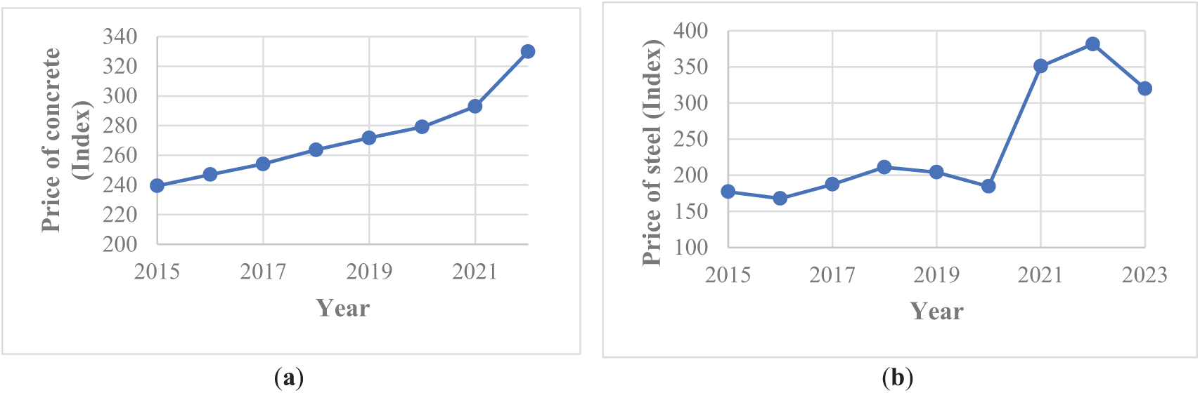
Figure 1: (a) US concrete product price [4] (b) Steel Price (US) [5]

Due to this trend of increasing prices, the need for optimal dimensioning of the RC retaining walls is highly significant from an economic point of view. The collapse or damage of retaining walls can cause material loss and, most importantly, the loss of life. In the design of these structures, both economically feasible and safe design are vital parameters. Depending on the intended use of the structure, the structure should be sized most safely and economically.

In this context, the aim of the study was determined to minimize the material costs of both concrete and reinforcing steel (required for the construction of the RC retaining wall) while ensuring its’ structural safety. The study methodology involved the optimization of design variables using the Flower Pollination Algorithm (FPA) to achieve a minimum-cost design. As a result of this optimization process, a dataset of possible solutions was generated. An ANN model was later developed based on this dataset to estimate the design variables. The following provides a summary of key examples from the previous research to better explain the use of optimization, artificial intelligence (AI), and machine learning (ML) in civil and structural engineering:

Optimization in Structural Engineering: Optimization is frequently used in structural design problems to minimize cost, weight, material usage, and carbon emissions. Some examples of the latest research include the following. Huang et al. [6] achieved the torsional design of carbon fiber-reinforced plastic concrete-filled steel tube columns using a data-driven optimization approach. Abo-Bakr et al. [7] used multi-objective particle swarm optimization (MOPSO) to minimize the mass and material cost of the irregular microbeams and maximize the critical buckling load and fundamental frequency. He et al. [8] performed parameterized multi-objective seismic optimization for a precast concrete frame with a beam-column joint with tension energy dissipation. Yu et al. [9] performed weight optimization of a thin-walled bamboo-like tubular beam subjected to bending. Zhao et al. [10] optimized hollow prismatic struts. Ocak et al. [11] investigated the response of the structure under near-fault earthquakes by hybrid use of the seismic isolator and tuned fluid damping device using the adaptive harmony search algorithm (AHS). Islam and Liu [12] conducted topology optimization of fiber-reinforced structures. Habashneh et al. [13] performed optimization of the advanced elastoplastic topology of steel beams at elevated temperatures using bidirectional evolutionary structural optimization (BESO). Aydın et al. [14] performed parameter optimization of the Tuned Mass Damper Inertia using Adaptive Harmony Search (AHS). Patil et al. [15] performed the optimization of a shift in the natural frequency of a nitinol-reinforced composite beam using the Technique for Order of Preference by Similarity to the Ideal Solution (TOPSIS). Mao et al. [16] used reliability-based topology optimization (RBTO) as a probabilistic-ellipsoid hybrid reliability multi-material topology tension constraint-based optimization method. Fu et al. [17] used a Jellyfish Search Optimizer (JSO) in the spreader optimization of the wide-span corridor bridge.

AI for Civil and Structural Engineering: Recently, artificial intelligence (AI) has been used for different purposes in civil and structural engineering including, structural analysis [18] crack detection [19], soil classification [20], RC beam-column model parameter prediction [21], prediction of maximum tensile stress in plain-weave composite laminates [22], evaluation of shear capacity of corroded reinforced concrete beams [23], shear strength prediction of RC beams [24], optimum design of reinforced concrete columns [25], prediction of concrete porosity using [26], seismic fragility and seismic vulnerability assessment of reinforced concrete structures [27], prediction of alkali-activated concrete carbon emissions [28], prediction of high-performance concrete compressive strength [29], predicting punching shear strength of fiber-reinforced concrete (FRC) flat slabs [30], failure mode classification model for RC columns [31], compressive strength prediction of ultra-high-performance concrete [32], modeling soil behavior [33], prediction of steel column stability with uncertain initial defects [34], detection of surface defects of civil structures using images [35].

Machine Learning for Civil and Structural Engineering: Most of the studies in the field of AI for Civil and Structural Engineering are focused on the use of machine learning. For instance, Bekdaş et al. [36] used machine learning-based prediction models to minimize the cost of RC retaining walls. Among the models they used, CatBoost achieved the highest success (R2 = 0.89). Cakiroglu et al. [37] used ensemble machine learning algorithms in the optimal design of cantilever soldier pile retaining walls to minimize total cost. The ensemble models they used obtained applicable results alternative to traditional models. Lemus-Romani et al. [38] minimized the cost and CO2 emissions using reinforcement learning approaches and metaheuristic techniques. The results obtained showed that S-shaped transfer functions achieve robust results. Ren et al. [39] used different ML models to predict the maximum reinforcement loads from the external properties and internal material parameters of the RC retaining wall and reached the most effective result with an XGBoost model. Bekdaş et al. [40] generated a dataset with Harmony Search (HS) to predict the optimum dimensions of the post-tensioned concrete cylindrical wall. Ocak et al. [41] predicted the required damping capacity of the isolator structure using ML, compared it with the previously installed isolator capacity, and determined the reduction in damping characteristics. They then trained machine learning models using this dataset and obtained high R2 values. Bui et al. [42] performed the prediction of the shear bond strength of asphalt concrete pavement using ML models. As a result of the study, they obtained effective prediction performance.

2  Materials and Methods

The analysis and design of RC retaining walls, which are widely used in practice, is an important challenge in engineering. Stability controllers should be utilized to evaluate the stability of RC retaining walls. The design of the cost-effective reinforced concrete retaining wall is affected by many parameters, such as foundation soil properties, wall properties, and unit cost. This study focuses on discovering the parameters of a minimum-cost RC retaining wall design with ANNs to aid the cost-efficient design of RC retaining walls based on data generated by the optimization process, in which the effects of different backfill internal friction angles, surcharge loads, wall heights and passive resistances (in the front part of the wall) are considered separately.

In the first stage, the design variables of the wall (length of the heel (y1), length of the toe (y2), thickness of the stem (top) (y3), thickness of the stem (bottom) (y4), foundation base thickness (y5) and cost (y6)) were optimized using Flower Pollination Algorithm (FPA) to minimize the material costs of both concrete and reinforcing steel, while ensuring its’ structural safety. As a result of this optimization, a dataset of 261,407 rows was generated. An ANN model was later developed based on this dataset to estimate the design variables, i.e., length of the heel (y1), length of the toe (y2), thickness of the stem (top) (y3), thickness of the stem (bottom) (y4), foundation base thickness (y5) and cost (y6) based on the height of the wall -H- (x1), material unit weight (x2), wall friction angle (x3), surcharge load (x4), concrete cost per m3 (x5), steel cost per ton (x6) and the soil class (x7). Fig. 2 is a simple representation of an RC retaining wall and depicts geometry-related variables. The following sections cover the details of the methodology.

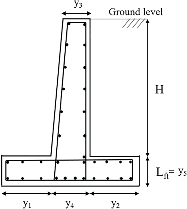
Figure 2: Geometry-related variables in the reinforced concrete retaining wall

2.1 Design of RC Retaining Walls

Turkey is in an earthquake zone, and seismic loads are taken into account when designing buildings. In addition, retaining structures must also be built earthquake-resistant. For this reason, reinforced concrete retaining walls are utilized to prevent the spread of the ground and to ensure the health of the structure. More realistic and up-to-date calculation methods were employed to obtain a more economical design of retaining walls utilized to prevent the spread of the ground.

Fig. 3 shows the design variables and typical forces acting on the reinforced concrete retaining wall. H is the wall height, h is the excavation depth, d is the embedment depth, γ1 is the backfill unit volume weight, φ1 is the internal friction angle, Lft is the foundation base thickness, Lh is the foundation heel width, Lsb is the body width at the foundation base level, and Ls is the body width at the ground level. Weights are Wws (wall body), Wfb (foundation base), Wsb and Wsf (retained soil at heel and footing), qa (uniformly distributed additional load). Pa and Pp (active and passive soil thrusts), Pqa and Pqae (forces from seismic additional loads). Ptb is the final value of the base pressure. Pase and Ppse are the active and passive earth pressures in the seismic case. Based on the Turkey Building Earthquake Regulation (TBER-2018) [43], the horizontal static-equivalent earthquake coefficient (kh) and vertical static-equivalent earthquake coefficient (kv) are given in Eqs. (1) and (2).

kh=0.4×SDSr(1)

kv=0.5×kh(2)

where r is the structural behavior coefficient for retaining structures, and its value varies based on the type of retaining structure, while SDS is the short-period design spectral acceleration coefficient. The value of SDS varies based on soil classes as specified in TBER-2018 [43].

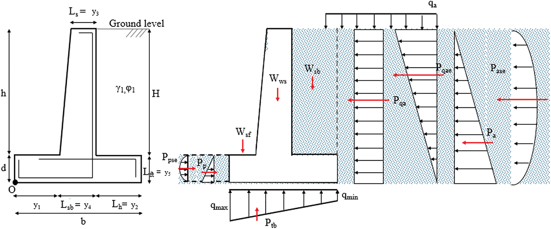
Figure 3: Design variables of reinforced concrete retaining wall and typical forces acting on a RC retaining wall

β is the slope of the soil surface behind the wall. φd′ is the shear strength angle of the soil. For β ≤ φd′ − θ, the dynamic active earth pressure coefficient (Ka) is calculated by Eq. (3).

Ka=sin2(ψ+∅d′−θ)cosθsin2ψsin⁡(ψ−θ−δd)[1+sin⁡(∅d′+δd)sin⁡(∅d′−β−θ)sin⁡(ψ−θ−δd)sin⁡(ψ+β)]2(3)

The dynamic passive pressure coefficient Kp is calculated by Eq. (4), assuming no friction between the floor and the wall.

Kp=sin2(ψ+∅d′−θ)cosθsin2ψsin⁡(ψ+θ)[1−sin⁡(∅d′)sin⁡(∅d′+β−θ)sin⁡(ψ−θ−δd)sin⁡(ψ+β)]2(4)

where ψ is the slope of the back face of the wall to the vertical; δd is the angle of the wall friction.

The total thrust acting on the retaining wall is calculated by Eq. (5).

Pt=K(1±kv)(12γ∗H2+qH)+Pwater+ΔPwater(5)

Based on TBER 2018, if the water level is below the foundation base level (Psu = ΔPsu = 0), the seismic angle (θ) is calculated by Eq. (6).

θ=tan−1[kh1±kv](6)

In the design of retaining walls, it is a good practice to perform overturning, sliding, and total collapse controls of the retaining wall first. Reinforced concrete section calculations are made after the positive results are obtained from these controls. In the sliding and overturning control of the retaining wall, it is accepted that the wall and groundmass on the base ground move together, and the overturning will occur by rotation around the lower front corner of the retaining wall [3].

(a)   In determining the safety of a reinforced concrete retaining wall against overturning, the total moments (∑MR) resisting overturning around the nose of the wall (point O in Fig. 3) are compared to the total moment (∑MO) of the forces attempting to overturn the wall (Eq. (7)).

SFoverturning=∑MR∑MO≥2.5(7)

The safety factor (SF) against overturning calculated by Eq. (7) must be greater than 2.5 for the static case.

(b)   The control of the safety of the retaining wall against sliding horizontally. It is assumed that the wall and the ground mass on the base floor move together. The safety factor against shear failure is calculated as the ratio of the sum of the shear resisting forces (∑FR) to the sum of the sliding forces (∑FS) in Eq. (8).

SFsliding=∑FR∑Fd≥1.5(8)

Eq. (8) must be satisfied for sliding control.

Vth≤Rth+0.3Rpt(9)

where Rth is the design frictional resistance, Rpt is the design passive resistance, and Vth is the design horizontal force.

(c)   In weak soils, the retaining wall and the ground mass can slide together, and complete collapse can occur. The vertical stresses acting on the wall should be transferred to the ground through the foundation to ensure safe bearing. Due to the eccentricity (e), the maximum and minimum base pressures occur at the heel and toe, respectively, and are assumed to vary linearly, as shown in Fig. 3.

Eq. (10) must be satisfied for the bearing capacity control of the foundation.

0<qmin;qmax<qa(10)

where qmin is the minimum base pressure under the foundation base, qmax is the maximum base pressure under the foundation base, and qa is the allowable bed pressure. qmin and qmax can be calculated as in Eq. (11).

qmax,min=∑VB(1±6eB)(11)

where ΣV is the weight of the wall, the sum of the soil and additional load on the base, i.e., the sum of the vertical forces. B is the width of the base. The calculation of the eccentric e is given in Eq. (12).

e=B2−∑MR−∑MO∑V(12)

It is recommended that the minimum reinforcement ratio and reinforcement spacing be placed in the retaining wall to meet the conditions in Eqs. (13) and (14), respectively.

ρ≥ρmin=0.003(S220);0.002(S420,S500)(13)

s≤smax=max[1.5hf;200mm)(14)

where hf is the plate thickness [3].

For cantilever retaining walls, it is recommended to follow the rules in Eqs. (15) and (16) for the placement and spacing of distribution reinforcement perpendicular to the main reinforcement.

As,distribution≥As,main/5(15)

s≤smax=300 mm(16)

2.2 Data Generation Process with Flower Pollination Algorithm (FPA)

Given the need for efficient resource utilization today, traditional structural design methods, which rely on trial and error, can not yield economical designs, highlighting the need for more optimized approaches. The conventional structural design process focuses on optimizing safety and cost-effectiveness. It strives to ensure safety while minimizing expenses, which often require significant effort and resources. Choosing the dimensions that will be sufficient for the cross-section to carry the load ensures that the structure is safe, but in this case, the structure can become uneconomical. The structure must be safe and economically viable. Optimization procedures aim to find the most suitable solution that minimizes costs without compromising safety.

In the optimum design, an economic design can be realized within the constraints. In optimization, design variables and limits, as well as function and structural constraints determined by the regulations in force, are defined by the user. Thus, when the maximum number of iterations is met, the results obtained from the structural analysis meet the constraints, and the optimum result is determined.

In recent years, metaheuristic methods have frequently been preferred for solving optimization problems. Unlike other methods used in optimization problems, many of the meta-heuristics are inspired by nature. Examples of these methods include (but are not limited to) the flower pollination Algorithm (FPA) [44] and the Honey Badger Algorithm (HBA) [45].

Flower Pollination Algorithm (FPA) is a mathematical model of pollen transfer for pollination of flowers. As in many other metaheuristic algorithms, the FPA has global and local search phases. The pollination of flowers requires biotic pollinators (flies, bees, and others) and abiotic pollinators (water, wind). The pollination process in flowers takes two different forms. Self-pollination is pollination between the pollen of the same plant species. Cross-pollination is pollination that occurs using pollen from more than one flower [44].

Since biotic pollinators can fly, they can carry pollen over long distances, ensuring the best reproduction. The expression for the floral constant is given in Eq. (17).

Xit+1=Xit+L(Xit−X∗)ifsp>r1(i=1,2,…,m)(17)

where Xit + 1 is the solution vector, X* is the current best vector, and t is the iteration counter.

The movement of insects over long distances can be expressed by the Lévy distribution. The Lévy distribution is shown in Eq. (18).

L=(12π)×r−1.5×e(12r)(18)

Local pollination can be formulated by Eq. (19).

Xit+1=Xit+ε(Xia,t−Xib,t)ifsp≤r1(19)

where xia,t and xib,t are the types of pollen that come from different flowers of the same plant species. ε is determined based on the uniform distribution [0, 1]. The prominent feature of this algorithm is the search for many solution points in the search space thanks to the Levy distribution [44].

The cost of the reinforced concrete retaining wall is the objective function f(x) as shown in Eq. (20).

minf(x)=Cc∗Vc+Cs∗Ws=(Cc∗L∗b∗h)+(Cs∗γs∗L∗As)(20)

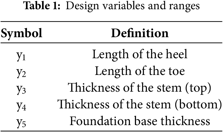
where L is retaining wall length, b is section width, h is the height of the section, Cc is concrete m3 unit cost, As is reinforcement cross-sectional area, γs is steel unit volume weight, Cs is steel m3 unit cost.

The lower and upper limits of the design variables are given in Table 1.

FPA is used for civil engineering optimization problems such as the optimization of RC frames [46], RC walls [47], and slope stability analysis [48]. Since FPA is adaptive and scalable, it outperforms other meta-heuristic algorithms in solving real-life optimization challenges [49]. Therefore, FPA was used in this study to achieve the best performance. This study aims to generate a new dataset and contribute to scientific literature. Thus, the study generated the used dataset.

Training and test data are needed for construction to estimate the variables required for the most economically feasible design of the retaining walls with ANNs, as well as to train and evaluate the model. This study generated the dataset for this purpose through the optimization process completed in MATLAB [50]. The dataset consisted of 261,407 lines and was in CSV format. All columns and rows in the dataset were numeric.

2.3 Exploratory Analysis of the Dataset

The data generated through the optimization was not subjected to any pre-processing. There are 7 input and 6 output variables in the data set. Input variables and their statistical features are given in Table 2. Table 2 shows the statistical properties of the inputs, and the abbreviations are the height of the wall (x1), material unit weight (x2), wall friction angle (x3), surcharge load (x4), concrete cost per m3 (x5), steel cost per ton (x6) and soil class (x7).

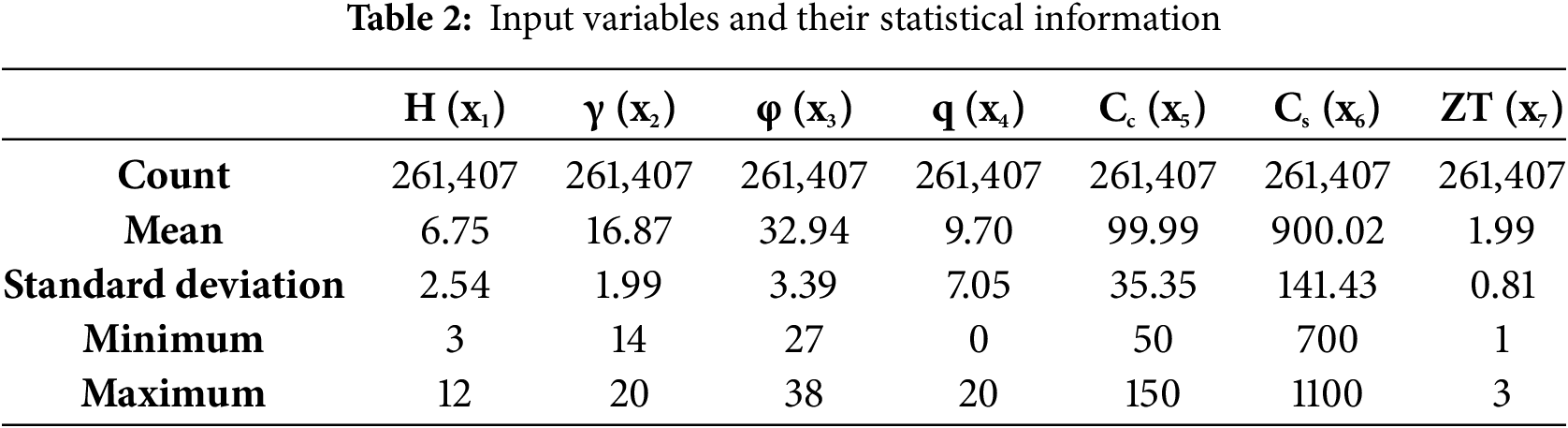
Table 3 shows the statistical properties of the outputs, and the abbreviations are length of the heel (y1), length of the toe (y2), thickness of the stem (top) (y3), thickness of the stem (bottom) (y4), foundation base thickness (y5) and cost (y6).

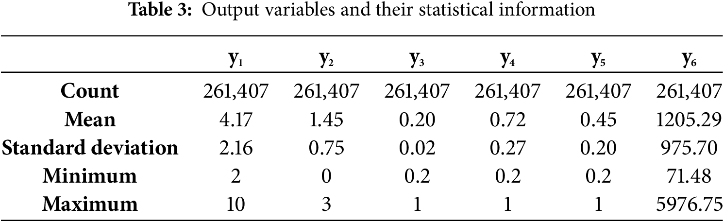
Statistical information of each input and output are listed in Tables 2 and 3. Histogram plots of inputs and outputs are also given to support these. Fig. 4 shows the histogram plots of output variables. The length of the heel (y1) output takes values between 2 and 10 and has a mean value of 4.17. The length of the toe (y2) output has a value between 0 and 3 and has a mean value of 1.45. The thickness of the stem (top) (y3) output has values between 0.2 and 1 and is clustered at 0.2. The thickness of the stem (bottom) (y4) output has values between 0.2 and 1, and values are similar to each other. The Foundation base thickness (y5) takes values between 0.2 and 1. Cost (y6) has taken values between 71.48 and 5976.75 and is mostly clustered around 1200.

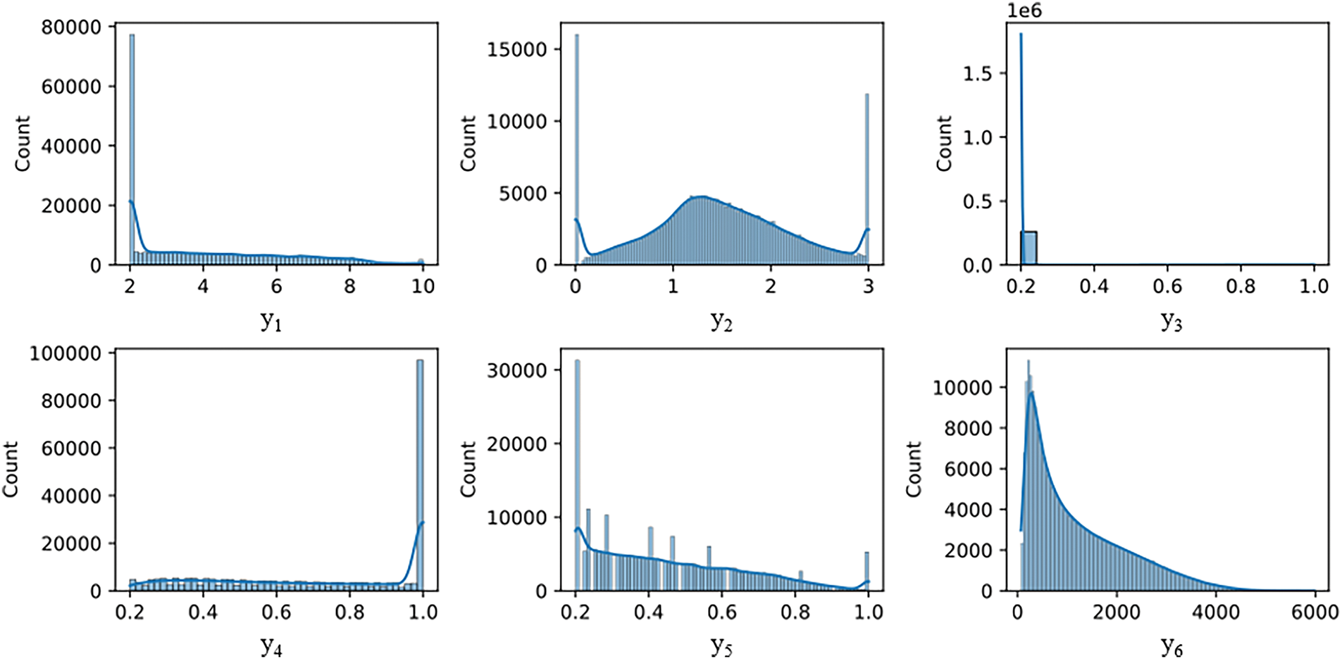
Figure 4: Histogram plots of output variables

Fig. 5 shows the histogram plots of input variables. It indicates that the distribution of inputs is uniform and not clustered at a certain value. Fig. 6 shows the correlation matrix of the dataset. In the matrix in Fig. 6, light colors represent high correlation, and dark colors represent low correlation. Cells of blue color in Fig. 6 indicate a high correlation, and cells of red color represent a weak correlation. The highest correlation is observed between the height of the wall (x1) and the foundation base thickness (y5). Neural networks are used because the presence of inputs with low correlation with outputs indicates that the data can contain non-linear relationships.

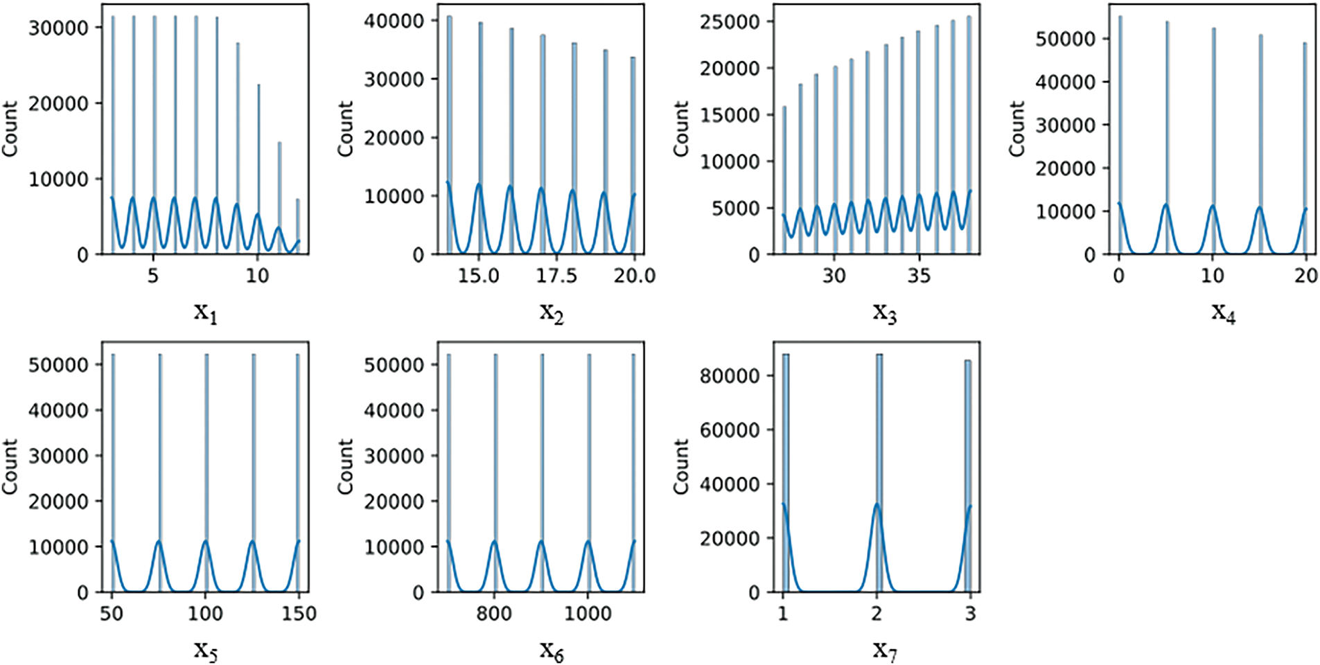
Figure 5: Histogram plots of input variables

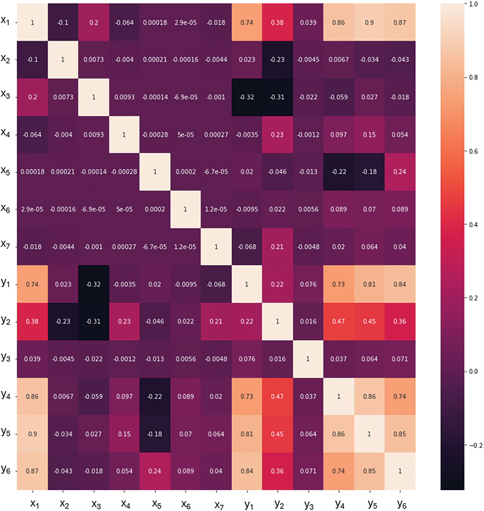
Figure 6: Correlation matrix of the dataset

2.4 Development of the Predictive Model

2.4.1 The Keras Library

Keras [51], one of the deep learning libraries for Python language, was used in the study. Keras enables running on both the Central Processing Unit (CPU) and Graphics Processing Unit (GPU) without modifying the code. Many different network structures can be implemented on Keras. Keras can be used free of charge. Google and Netflix are among the companies using Keras [52]. Keras’ writing language is easy and descriptive.

In Keras, the ANN model is created and then trained using the training data. Once the model is trained, the model is utilized to make inferences about the test data. In a Keras model, the model is first defined, and layers are added. The compilation method configures the model by specifying losses, optimizers, and measurements. Finally, the fit method is called to train the model. The Keras-based workflow in this study is illustrated in Fig. 7.

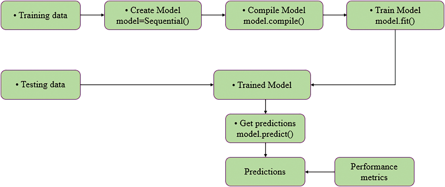
Figure 7: Keras based workflow

Sequential, a type of Keras model for stacking network layers, was utilized in this study. The other components utilized to create the network are provided below.

2.4.2 Model Structure

Activation Function

Activation functions determine how the outputs produced in the sum function of neurons change. This study chooses the Rectified Linear Unit (ReLU) as the activation function for both hidden layers. ReLU is a non-linear activation function that can perform derivative operations. ReLU is widely used in ANN designs because it overcomes the vanishing gradient problem and has a low computational load [53]. Fig. 8 exhibits that the ReLU activation function returns 0 for negative values and an input value for positive values.

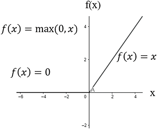
Figure 8: ReLU activation function [54]

Loss Function

Loss functions are mathematical functions that calculate how far the model’s predictions are from the true values during the training of deep learning models. These functions are utilized to evaluate the performance of the model and help the adjustment of weight updates in the training process [55]. In this study, the mean squared error (MSE) is chosen as the loss function. MSE is one of the most widely used loss functions and is particularly favored in regression problems. MSE compares the prediction of the model with the actual values and calculates the mean of the error squares for each sample. MSE is calculated by Eq. (21).

MSE=1N∑i=1N(yi−yi^)2(21)

where N is the total number of data, yi is the true value, and yi^ is the predicted value.

Optimization Algorithms (Optimizers)

Optimization algorithms help the ANN model to perform better by minimizing the loss function of the model. These algorithms use gradient descent and derivative-based techniques to update the model weights [55]. This study chooses Adam as the optimizer. Adam is a derivative of the gradient descent algorithm and works more quickly and efficiently. This algorithm updates the weights using adaptive momentum and adaptive learning rate [55].

Model Evaluation Metrics

There are many metrics for measuring and evaluating the performance of algorithms and models. It can be understood whether the proposed model or system provides the solution to the current design by looking at these metrics. This study uses the Coefficient of Determination (R2), Mean Squared Error (MSE) (Eq. (21)), and Root Mean Squared Error (RMSE) to evaluate the performance of the model.

The coefficient of determination provides the ratio of variance explained by the model to the total variance in the dataset. R2 can be utilized to measure the model performance in certain regression models (Eq. (22)).

R2=VarianceexplainedbythemodelTotalvariance(22)

The root mean squared error is determined by taking the sum of squares of models’ errors and taking the square root of this sum (Eq. (23)). RMSE is a very widely used error metric regression type problem.

RMSE=1N∑i=1N(yactual−ypred)2(23)

2.5 Model Implementation

This study utilizes the Keras ANN framework and the Keras Sequential model to estimate the design variables of the RC retention walls based on input variables that are provided as the result of the FPA-based optimization process. The trained ANN model has 1 input, 2 hidden, and 1 output layer. The structure of the ANN is shown in Fig. 9.

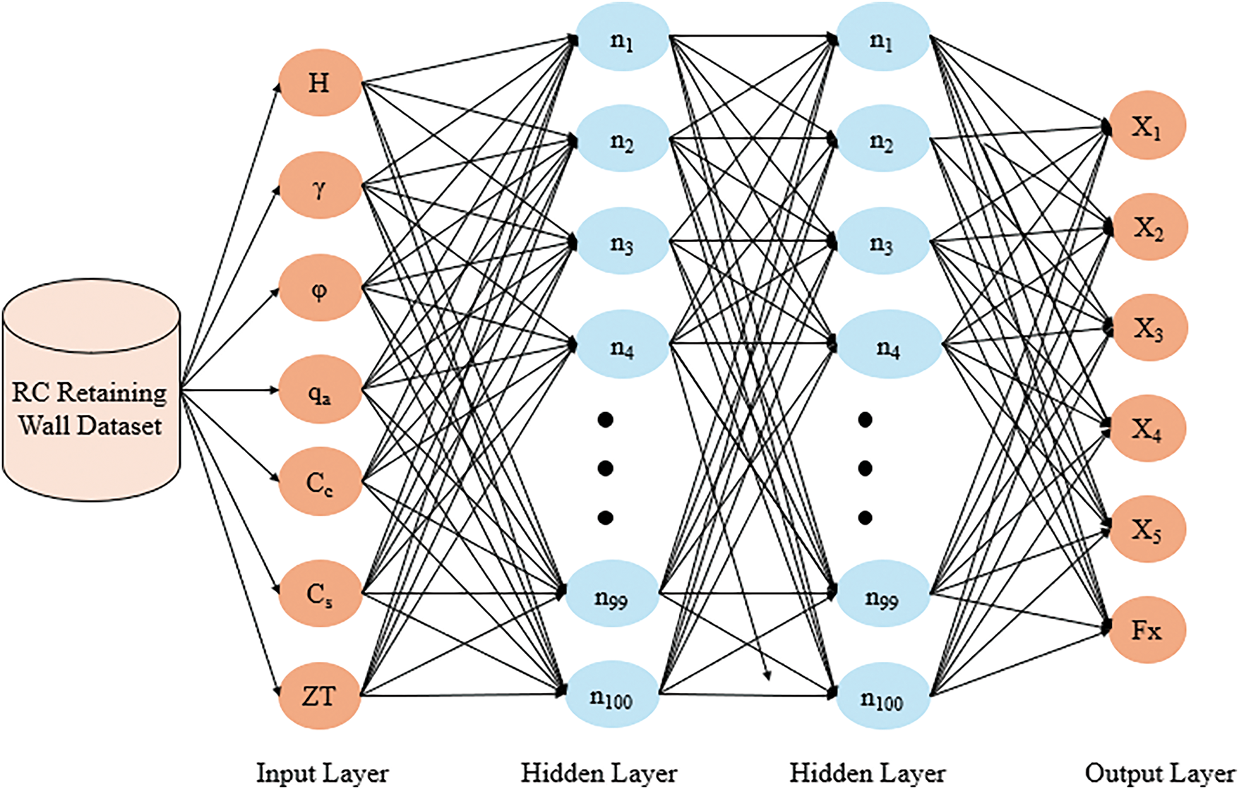
Figure 9: Artificial Neural Network for RC Retaining Wall Dataset

Fig. 9 indicates that the hidden layers in the network correspond to a series of consecutive functions. They are connected to the previous and the next one until they reach the output layer. The data set is fed from the input layer. The output layer provides the desired output (estimation). This study utilizes the ANN with an input layer of size 7, two hidden layers with size of 100, and the output layer with a size of 6. The ReLU activation function is used in hidden layers, the loss function of the network is MSE, and the optimizer of the model is Adam. The model is evaluated with multiple metrics, including R2 and RMSE.

2.6 Model Interpretation with Explainable AI (XAI)

The accuracy/precision of the results of ANNs can be assessed using various metrics. However, these algorithms behave as opaque systems that process data and deliver output. This opacity has sparked interest in the mechanisms underlying these processes, prompting the development of explainable artificial intelligence techniques [56]. Explainable artificial intelligence (XAI) techniques enable humans to interpret and understand the results. The need for explainable artificial intelligence also varies depending on the target of artificial intelligence and the field in which it is applied. The XAI techniques used in this study were Local Interpretable Model-agnostic Explanations (LIME) and SHapley Additive exPlanations (SHAP).

2.6.1 LIME (Local Interpretable Model-Agnostic Explanations)

LIME is a visual technique that can be applied to any machine learning algorithm in general. It is proposed that the model be explained by approximating model predictions to an interpretable model [57]. This technique assumes that “Every complex model is linear at the local scale”. It can be summarized as deriving new observations with characteristics similar to the observations in the data set and revealing the effects and importance of explanatory variables on prediction. The LIME output summarizes the contribution of the explanatory variables to the prediction of the selected observations and allows finding the explanatory variables that have the most impact on the prediction. The method describes the algorithm by understanding how the prediction changes for a given single sample and is, therefore, suitable for localized explanations [58]. The purpose of using LIME is to increase the interpretability and explainability of the models.

2.6.2 SHAP (SHapley Additive exPlanations)

SHAP (SHapley Additive Explanations) is another method of explainable artificial intelligence and allows interpretations to be made on an artificial intelligence model. The SHAP study was published by Lundberg and Lee in 2017 [56]. SHAP is a game-theoretic method for describing the performance of a model. In SHAP, an output model is defined as a linear sum of input variables [59].

Although SHAP can display results both locally and globally, LIME produces one plot per instance. In the study, both SHAP and LIME were utilized together to make the explanatory process of the models more robust and comprehensive.

2.7 Summary of Methodology

The methodology of the study is briefly summarized in Fig. 10 to make the overall study clear and understandable.

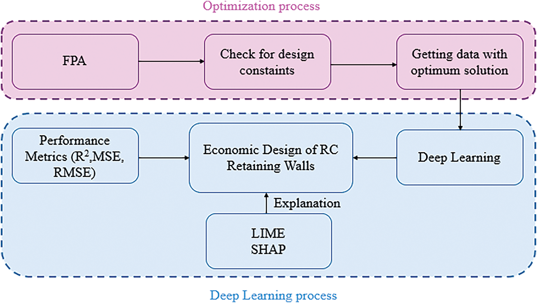
Figure 10: The overall process of study

Fig. 10 indicates that the study started with an optimization process focused on finding the most economically feasible design using the FPA algorithm. In the optimization process, design constraints were considered to minimize the objective function (cost), and a dataset providing the possible combinations of attributes of wall and soil (x1, …, x7) and design variables (y1, …, y6) was obtained. This dataset was then used as input for the ANN model to estimate the possible values of design variables of the most economically feasible (and structurally viable) RC retaining wall. Finally, evaluation metrics were utilized to evaluate the success of the ANN model, and the explanations of the model features’ impact on the outputs were determined using the Explainable Artificial Intelligence (XAI) methods.

3  Results

Python programming language and Spyder IDE (open-source development environment) were utilized to evaluate the ANN model and Explainable Artificial Intelligence (XAI) methods. For the model development and evaluation process, the dataset was divided into two training and test sets. The performance of the ANN model in the training and testing phases is evaluated based on the R2 and RMSE values at each epoch. The graphs in Figs. 11 and 12 provide these values for the training and the test set.

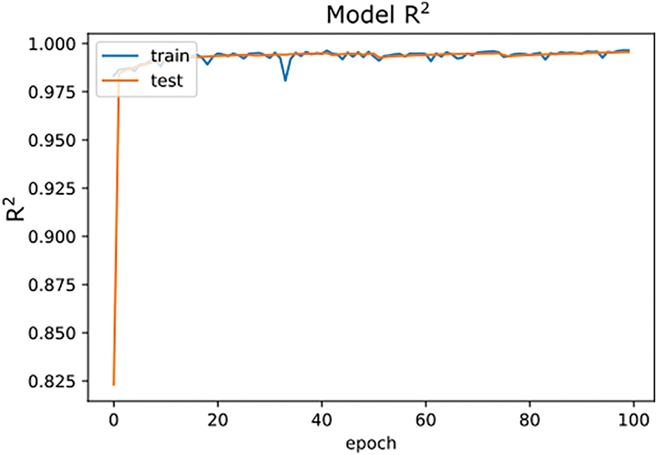
Figure 11: R2 of model for 100 epochs

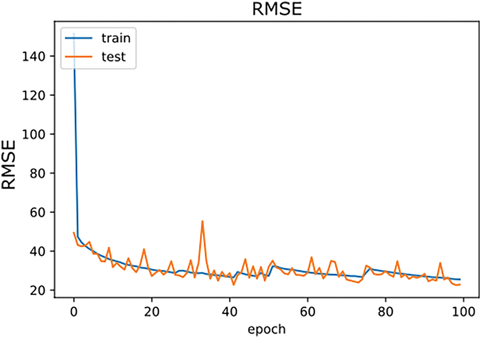
Figure 12: RMSE of model for 100 epochs

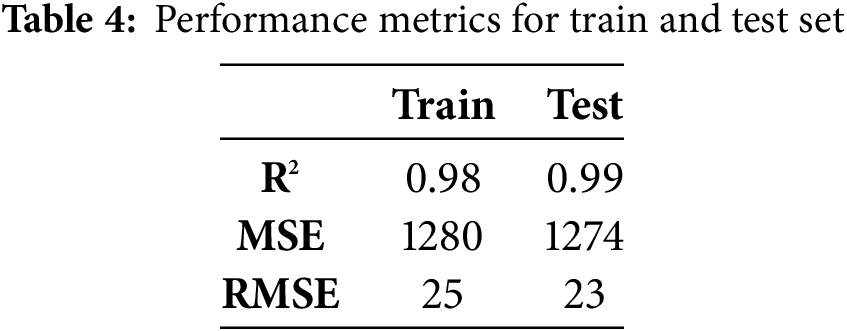
The evaluation metrics in each epoch were examined to detect the optimal number of epochs for the model’s training. Figs. 11 and 12 illustrate that an R2 value of 0.99 was reached after the 7th epoch. The model with the same features was run 50 times repeatedly to validate the results, and similar results were observed in each run. In epochs 1 to 100, the RMSE value ranged between 49 and 23, as shown in Fig. 12. Finally, the MSE value was 1274.0774, the RMSE value was 23.7357, and the R2 value was 0.9962 at epoch 100. The model was able to provide accurate results with a high R2 value (>0.99) when the training was finished. Table 4 shows the neural network performance metrics for training and test sets.

In the scatter plots representing the relationship between ground truth and predicted values, if there is no regular clustering on the regression curve, it means that the relationship between these two features is weak or non-existent, and if there is a regular distribution, it indicates a strong relationship between the two features. The target variables in Fig. 13, y1 denotes the length of the heel, y2 indicates the length of the toe, y3 is the thickness of the stem (top), y4 indicates the thickness of the stem (bottom), y5 is the foundation base thickness, and y6 indicates the cost.

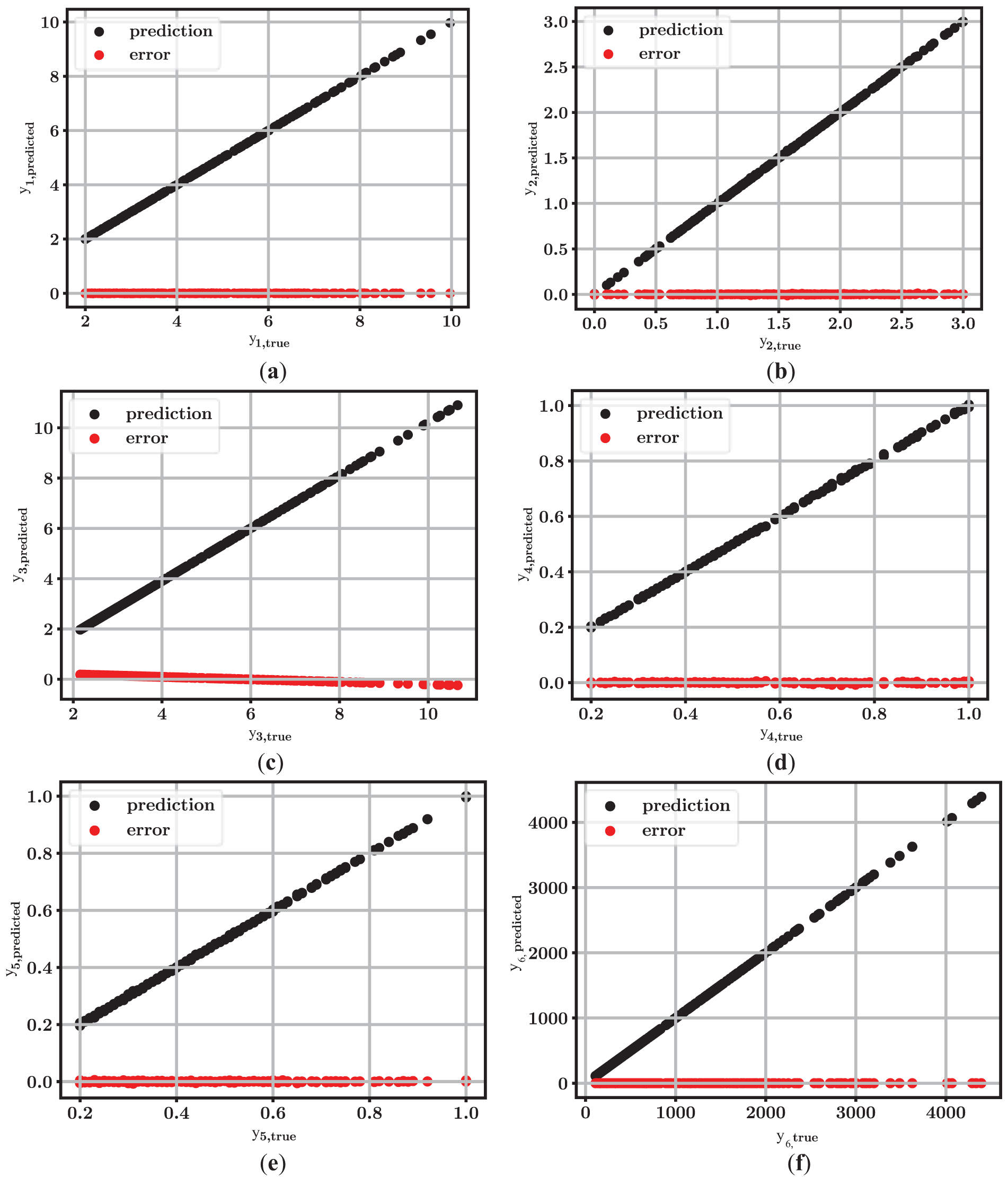
Figure 13: Scatter plots for each output (a) y1, (b) y2, (c) y3, (d) y4, (e) y5, (f) y6

When the scatter plots in Fig. 13 are analyzed, the predictions for target variables appear to be very successful. Specifically, the most successful prediction among the outputs is the cost (y6) prediction, and the weakest prediction is the length of the heel (y1) prediction. Fig. 14 illustrates the LIME outcome for each output. For each output, LIME is applied using the input values from row 5 of the dataset to ensure equal observations. The input (feature) values are the height of the wall (x1), material unit weight (x2), wall friction angle (x3), surcharge load (x4), concrete cost per m3 (x5), steel cost per tonne (x6) and soil class (x7). In Fig. 14, H represents x1, γ represents x2, φ represents x3, q represents x4, Cc represents x5, Cs represents x6, and ZT represents x7.

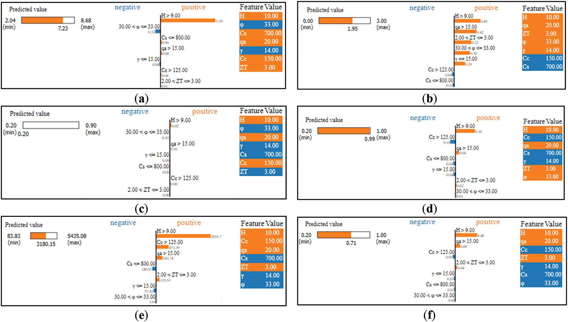
Figure 14: The LIME outcome for each output (a) y1, (b) y2, (c) y3, (d) y4, (e) y5, (f) y6

Fig. 14a indicates that the model’s prediction for the length of the heel (y1) is 7.23. H > 9, Cs ≤ 800, q > 15, Cc > 125, and 2.00 < ZT ≤ 3 values positively correlate with the prediction of the length of the heel. Fig. 14b demonstrates that the deep learning model prediction for the length of the toe (y2) is 1.95. H > 9, q > 15, 2.00 < ZT ≤ 3, 30 < φ ≤ 33, γ ≤ 15 values positively correlate with the prediction of the length of the toe. Fig. 14c shows that the deep learning model prediction for the thickness of the stem (top) (y3) is 0.20. H > 9, q > 15, and Cc > 125 values positively correlate with the prediction of the thickness of the stem (top). Fig. 14d reveals that the deep learning model prediction for the thickness of the stem (bottom) (y4) is 0.99. H > 9, q > 15, 2.00 < ZT ≤ 3, and 30 < φ ≤ 33 values positively correlate with the prediction of the thickness of the stem (bottom). Fig. 14e demonstrates that the deep learning model prediction for the foundation base thickness (y5) is 0.71. H > 9, q > 15, and 2.00 < ZT ≤ 3 values positively correlate with the prediction of foundation base thickness. Fig. 14f indicates that the deep learning model prediction for the cost was 3180.15. H > 9, Cc > 125, q > 15, and 2.00 < ZT ≤ 3 values positively correlate with the prediction of cost (y6).

Fig. 15 shows the SHAP summary plots for all the output features. The dots in Fig. 15 are the data points in the data set, and the color of the dots is the value of the features. The figure shows the SHAP value distribution of the input features. The horizontal position of each point represents the influence of that feature on the output. Positive SHAP values of a feature indicate an increasing effect on the model output, whereas negative SHAP values indicate a decreasing effect [60]. The results of the SHAP analysis show that the H has the greatest impact on the length of the heel (y1), length of the toe (y2), thickness of the stem (bottom) (y4), thickness of the retaining wall foundation (y5) and cost (y6).

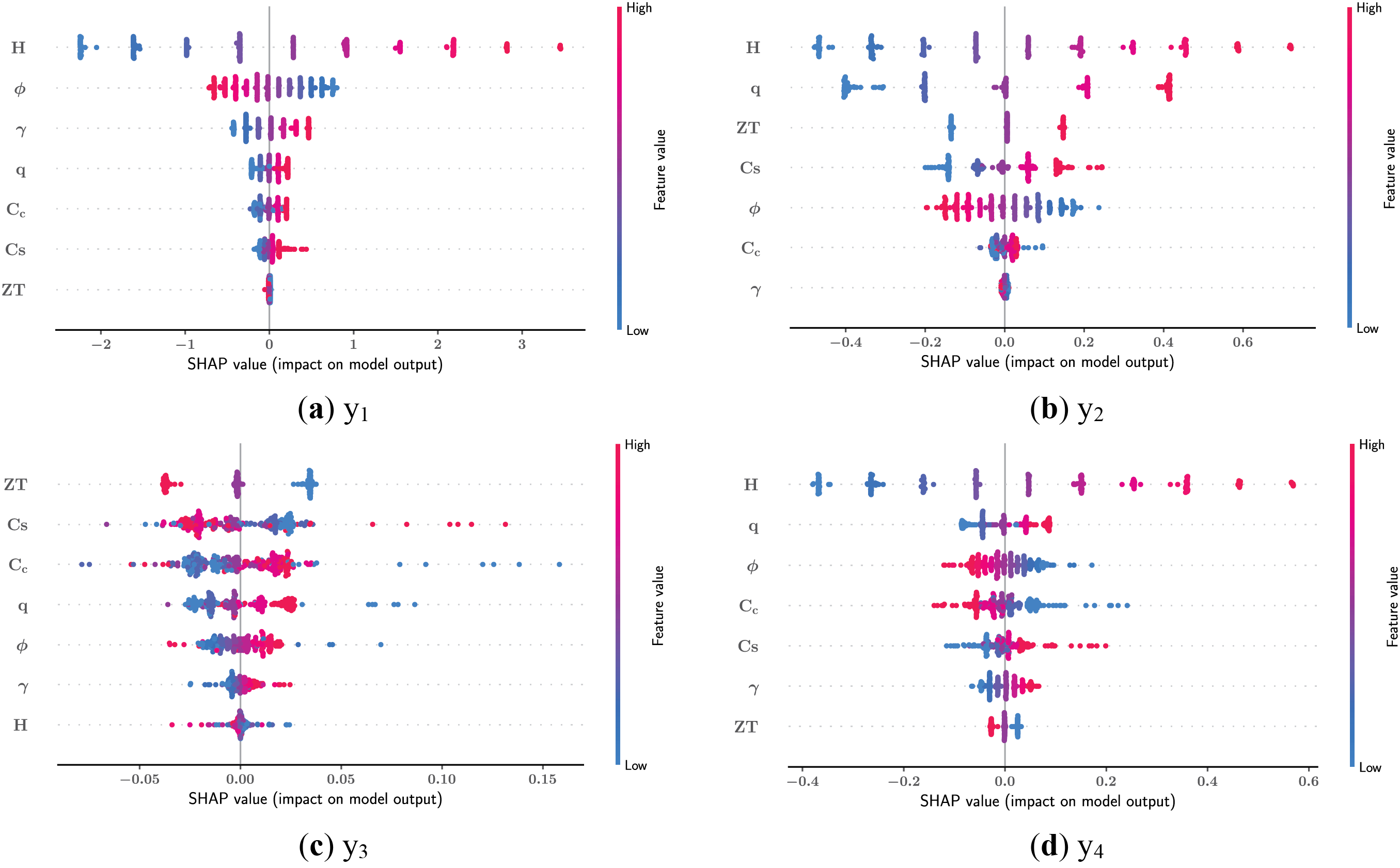
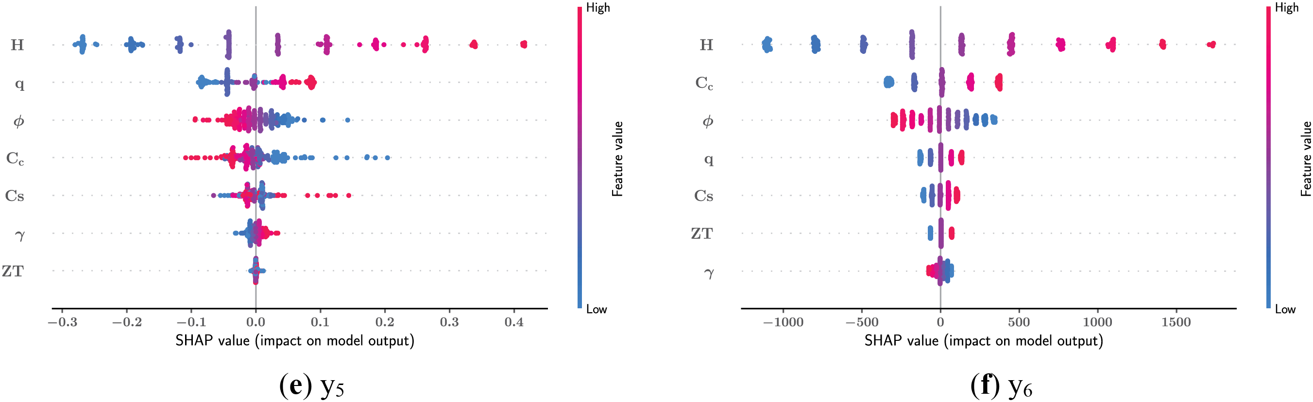
Figure 15: SHAP summary plots of the output features

An alternative representation of the feature impacts on the model outputs is depicted in Fig. 16 with heatmap plots. Each vertical line in Fig. 16 corresponds to one of the data points. In the heatmap plots, features with high impact have SHAP values with high magnitude and are shown in darker tones of red and blue. In contrast, features with low impact are represented with colors close to white. The feature importance is also shown along the vertical axis on the right-hand side with horizontal bars that visualize the mean absolute SHAP values of features. The value of the output feature is denoted with f(x), and its variation for each data point is plotted at the top of each heatmap plot. Fig. 16 shows that H is the most impactful feature in the prediction of all output features except for y3.

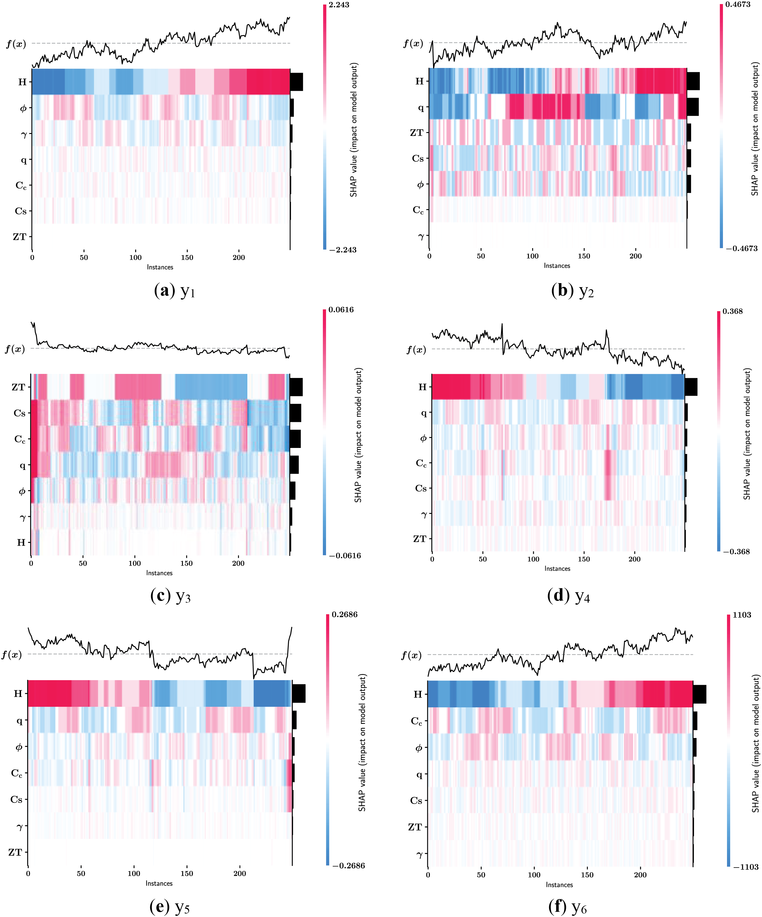
Figure 16: SHAP heatmap plots for the output features

4  Discussion

The application of optimization and artificial intelligence in structural engineering contributes to structural design. In this study, the cost and dimensional variables of a retaining wall are predicted using optimized retaining wall parameters. The present study uses a database of 261,407 rows for training neural networks. It was observed that the neural network models used have high accuracy in terms of R2, MSE, and RMSE. Neural networks can show high performance on large data sets. Since the data set is large and contains different combinations, the neural networks were able to generalize better thanks to their learning capacity. The variable H has the greatest importance in all outputs except y3 output. LIME plots also support this. When the results are analyzed, it is seen that neural networks have high prediction success. Based on all these results, it can be said that neural networks give excellent results in dimensioning and cost prediction of retaining walls.

Table 5 compares the results of this study with those predicted by the properties of the existing shear retaining wall. In these studies, mainly Random Forest (RF), Extreme Gradient Boosting (XGBoost), Categorical Gradient Boosting (CatBoost), and Light Gradient Boosting Machine (LightGBM) ML models were utilized. This study performs the prediction using an ANN developed with Keras, a deep learning framework.

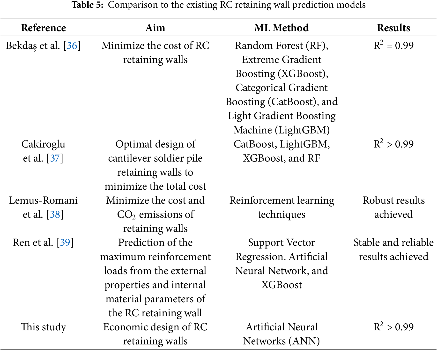
Table 4 shows that the use of data-driven methods to predict RC retaining wall properties is popular. The most used models are Random Forest (RF), Extreme Gradient Boost (XGBoost), Categorical Gradient Boost (CatBoost) and Lightweight Gradient Boost Machine (LightGBM). Table 4 indicates that the proposed methodology was able to achieve an R2 value of 0.99 using ANN. This study used standard computing resources (Intel(R) Xeon(R) CPU @ 2.20 GHz (Model: 79, Family: 6) and 32 GB RAM), and the training of 100 epochs took approximately 30 min; thus the model was not very time-efficient.

Accordingly, the cost-effective/economically feasible design of reinforced concrete retaining walls is essential since these walls are widely used retaining structures. The trial-and-error process for achieving cost-efficient designs takes a long time, and the success is limited to the engineer’s point of view and experience. This study aims to reduce the time and effort spent on the cost-effective design of retaining walls by making use of Artificial Neural Networks (ANNs).

5  Conclusions

This study uses an optimization algorithm coded by the authors based on the Flower Pollination Algorithm in MATLAB environment to generate a data set of 261,407 rows. This dataset is utilized to train an ANN model. The results showed that the ANN model provides an estimation of design variables with very high accuracy. Finally, Local Interpretable Model-Agnostic Explanations (LIME) and SHapley Additive Explanations (SHAP) methods increase the interpretability of the model and further highlight the relations and causality between the predictor and target variables.

The research confirms that the height of the wall, material unit weight, wall friction angle, surcharge load, concrete cost per m3, steel cost per ton, and soil class can be used in the cost-effective design of reinforced concrete retaining walls as input variables to a multi-output regression analysis to estimate the length of the heel, length of the toe, thickness of the stem (top), thickness of the stem (bottom), foundation base thickness and cost.

One of the main highlights of this work is the very high performance of ANN models in estimating the variables of the design with optimum cost and high accuracy for different situations using a large dataset.

Similar estimations will be made in the future with better confidence when black box models with high performance can be explained by Explainable Artificial Intelligence (XAI) approaches. The predictive power of deep learning models depends on the existence of large amounts of quality data. Therefore, when this type and amount of data becomes available for many other problems, ANNs can be used in different civil engineering problems through the implementation of similar methodological approaches.

Acknowledgement: The authors are highly supported by all reviewers and journal editors, and their valuable comments are very useful in improving our study.

Funding Statement: The authors received no specific funding for this study.

Author Contributions: The background and theory of the problem were developed by Gebrail Bekdaş, Yaren Aydın, and Umit Işıkdağ. Gebrail Bekdaş, Yaren Aydın, Celal Cakiroglu, and Umit Işıkdağ wrote the text. The analysis codes were generated by Gebrail Bekdaş, Yaren Aydın, and Celal Cakiroglu. Gebrail Bekdaş and Umit Işıkdağ verified the results. Yaren Aydın drew the figures, and Gebrail Bekdaş supervised Celal Cakiroglu’s Research direction. All authors reviewed the results and approved the final version of the manuscript.

Availability of Data and Materials: The data that support the findings of this study are available from the corresponding author upon reasonable request.

Ethics Approval: Not applicable.

Conflicts of Interest: The authors declare no conflicts of interest to report regarding the present study.

References

1. Önalp A. Geotechnical knowledge for civil engineers. Trabzon, Türkiye: Karadeniz Technical University; 1982. Vol. 2. [Google Scholar]

2. Tan Y, Lu Y, Wang D. Synchronous-cross zoned excavation of the oversized basement of Shanghai International Financial Centre by combination of bottom-up and top-down methods: structural and geotechnical behaviors. Tunn Undergr Space Technol. 2024;153(1):106023. doi:10.1016/j.tust.2024.106023. [Google Scholar] [CrossRef]

3. Celep Z. Introduction to earthquake engineering and earthquake resistant building design. İstanbul, Türkiye: Beta; 2019. [Google Scholar]

4. Statista. U.S. producer price index of concrete products from 1926 to 2023. [cited 2025 Jan 25]. Available from: https://www.statista.com/statistics/195544/us-producer-price-index-of-concrete-products-since-1990/. [Google Scholar]

5. IBISWorld. Recent trends—price of steel. [cited 2025 Jan 25]. Available from: https://www.ibisworld.com/us/bed/price-of-steel/112696/. [Google Scholar]

6. Huang H, Xue C, Zhang W, Guo M. Torsion design of CFRP-CFST columns using a data-driven optimization approach. Eng Struct. 2022;251(3):113479. doi:10.1016/j.engstruct.2021.113479. [Google Scholar] [CrossRef]

7. Abo-Bakr HM, Abo-Bakr RM, Mohamed SA, Eltaher MA. Weight optimization of axially functionally graded microbeams under buckling and vibration behaviors. Mech Based Des Struct Mach. 2023;51(1):213–34. doi:10.1080/15397734.2020.1838298. [Google Scholar] [CrossRef]

8. He Z, Gao M, Li Z, Guo Z, Ke S, Qi Z, et al. Parametrized multi-objective seismic optimization for precast concrete frame with a novel post-tensioned energy dissipation beam-column joint. Comput Struct. 2023;275(1):106911. doi:10.1016/j.compstruc.2022.106911. [Google Scholar] [CrossRef]

9. Yu Y, Ma D, Zhang L, Yang X, Guan H. Elastic buckling analysis and optimization of thin-walled bamboo-like pipe beam subjected to pure bending. Chin J Aeronaut. 2024;37(3):133–52. doi:10.1016/j.cja.2023.12.006. [Google Scholar] [CrossRef]

10. Zhao M, Li X, Zhang DZ, Zhai W. Design, mechanical properties and optimization of lattice structures with hollow prismatic struts. Int J Mech Sci. 2023;238:107842. doi:10.1016/j.ijmecsci.2022.107842. [Google Scholar] [CrossRef]

11. Ocak A, Bekdaş G, Nigdeli SM. Optimum design of hybrid base isolation and tuned liquid damper systems for structures under near-fault ground motions. ASCE ASME J Risk Uncertainty Eng Syst Part A Civ Eng. 2024;10(4):04024061. doi:10.1061/AJRUA6.RUENG-1357. [Google Scholar] [CrossRef]

12. Islam MM, Liu L. Topology optimization of fiber-reinforced structures with discrete fiber orientations for additive manufacturing. Comput Struct. 2024;301(1):107468. doi:10.1016/j.compstruc.2024.107468. [Google Scholar] [CrossRef]

13. Habashneh M, Cucuzza R, Domaneschi M, Movahedi Rad M. Advanced elasto-plastic topology optimization of steel beams under elevated temperatures. Adv Eng Softw. 2024;190:103596. doi:10.1016/j.advengsoft.2024.103596. [Google Scholar] [CrossRef]

14. Aydın Y, Bekdaş G, Nigdeli SM, Geem ZW. Parameter optimization of tuned mass damper inerter via adaptive harmony search. Comput Model Eng Sci. 2024;141(3):2471–99. doi:10.32604/cmes.2024.056693. [Google Scholar] [CrossRef]

15. Patil RA, Rane SB, Kumbhar SB. Optimization of a shift in the natural frequency of anitinol-reinforcedcomposite beam. Int J Interact Des Manuf. 2024;18(3):1761–75. doi:10.1007/s12008-023-01700-2. [Google Scholar] [CrossRef]

16. Mao Z, Zhao Q, Zhang L. Probabilistic-ellipsoid hybrid reliability multi-material topology optimization method based on stress constraint. Comput Model Eng Sci. 2024;140(1):757–92. doi:10.32604/cmes.2024.048016. [Google Scholar] [CrossRef]

17. Fu S, Wu X, Wang W, Hu Y, Li Z, Jiang F. An improved JSO and its application in spreader optimization of large span corridor bridge. Comput Model Eng Sci. 2024;138(3):2357–82. doi:10.32604/cmes.2023.031118. [Google Scholar] [CrossRef]

18. Wang C, Song LH, Fan JS. End-to-end structural analysis in civil engineering based on deep learning. Autom Constr. 2022;138(1):104255. doi:10.1016/j.autcon.2022.104255. [Google Scholar] [CrossRef]

19. Kalfarisi R, Wu ZY, Soh K. Crack detection and segmentation using deep learning with 3D reality mesh model for quantitative assessment and integrated visualization. J Comput Civ Eng. 2020;34(3):04020010. doi:10.1061/(ASCE)CP.1943-5487.0000890. [Google Scholar] [CrossRef]

20. Aydın Y, Işıkdağ Ü, Bekdaş G, Nigdeli SM, Geem ZW. Use of machine learning techniques in soil classification. Sustainability. 2023;15(3):2374. doi:10.3390/su15032374. [Google Scholar] [CrossRef]

21. Rayjada SP, Raghunandan M, Ghosh J. Machine learning-based RC beam-column model parameter estimation and uncertainty quantification for seismic fragility assessment. Eng Struct. 2023;278:115111. doi:10.1016/j.engstruct.2022.115111. [Google Scholar] [CrossRef]

22. Bagherzadeh F, Shafighfard T, Khan RMA, Szczuko P, Mieloszyk M. Prediction of maximum tensile stress in plain-weave composite laminates with interacting holes via stacked machine learning algorithms: a comparative study. Mech Syst Signal Process. 2023;195(1):110315. doi:10.1016/j.ymssp.2023.110315. [Google Scholar] [CrossRef]

23. Kumar A, Arora HC, Kapoor NR, Kumar K, Hadzima-Nyarko M, Radu D. Machine learning intelligence to assess the shear capacity of corroded reinforced concrete beams. Sci Rep. 2023;13(1):2857. doi:10.1038/s41598-023-30037-9. [Google Scholar] [PubMed] [CrossRef]

24. Sandeep MS, Tiprak K, Kaewunruen S, Pheinsusom P, Pansuk W. Shear strength prediction of reinforced concrete beams using machine learning. Structures. 2023;47:1196–211. doi:10.1016/j.istruc.2022.11.140. [Google Scholar] [CrossRef]

25. Aydın Y, Bekdaş G, Nigdeli SM, Isıkdağ Ü, Kim S, Geem ZW. Machine learning models for ecofriendly optimum design of reinforced concrete columns. Appl Sci. 2023;13(7):4117. doi:10.3390/app13074117. [Google Scholar] [CrossRef]

26. Cao C. Prediction of concrete porosity using machine learning. Results Eng. 2023;17(2):100794. doi:10.1016/j.rineng.2022.100794. [Google Scholar] [CrossRef]

27. Kazemi F, Asgarkhani N, Jankowski R. Machine learning-based seismic fragility and seismic vulnerability assessment of reinforced concrete structures. Soil Dyn Earthq Eng. 2023;166(7):107761. doi:10.1016/j.soildyn.2023.107761. [Google Scholar] [CrossRef]

28. Aydın Y, Cakiroglu C, Bekdaş G, Işıkdağ Ü, Kim S, Hong J, et al. Neural network predictive models for alkali-activated concrete carbon emission using metaheuristic optimization algorithms. Sustainability. 2024;16(1):142. doi:10.3390/su16010142. [Google Scholar] [CrossRef]

29. Islam N, Kashem A, Das P, Ali MN, Paul S. Prediction of high-performance concrete compressive strength using deep learning techniques. Asian J Civ Eng. 2024;25(1):327–41. doi:10.1007/s42107-023-00778-z. [Google Scholar] [CrossRef]

30. Liu T, Cakiroglu C, Islam K, Wang Z, Nehdi ML. Explainable machine learning model for predicting punching shear strength of FRC flat slabs. Eng Struct. 2024;301(4):117276. doi:10.1016/j.engstruct.2023.117276. [Google Scholar] [CrossRef]

31. Kim S, Hwang H, Oh K, Shin J. A machine-learning-based failure mode classification model for reinforced concrete columns using simple structural information. Appl Sci. 2024;14(3):1243. doi:10.3390/app14031243. [Google Scholar] [CrossRef]

32. Aydın Y, Cakiroglu C, Bekdaş G, Geem ZW. Explainable ensemble learning and multilayer perceptron modeling for compressive strength prediction of ultra-high-performance concrete. Biomimetics. 2024;9(9):544. doi:10.3390/biomimetics9090544. [Google Scholar] [PubMed] [CrossRef]

33. Bekdaş G, Aydın Y, Nigdeli SM, Ünver İS, Kim WW, Geem ZW. Modeling soil behavior with machine learning: static and cyclic properties of high plasticity clays treated with lime and fly ash. Buildings. 2025;15(2):288. doi:10.3390/buildings15020288. [Google Scholar] [CrossRef]

34. Zhao H, Wang C, Fan J. Predicting steel column stability with uncertain initial defects using Bayesian deep learning. Appl Soft Comput. 2024;151(4):111139. doi:10.1016/j.asoc.2023.111139. [Google Scholar] [CrossRef]

35. Guo J, Liu P, Xiao B, Deng L, Wang Q. Surface defect detection of civil structures using images: review from data perspective. Autom Constr. 2024;158(2):105186. doi:10.1016/j.autcon.2023.105186. [Google Scholar] [CrossRef]

36. Bekdaş G, Cakiroglu C, Kim S, Geem ZW. Optimal dimensioning of retaining walls using explainable ensemble learning algorithms. Materials. 2022;15(14):4993. doi:10.3390/ma15144993. [Google Scholar] [PubMed] [CrossRef]

37. Cakiroglu C, Islam K, Bekdaş G, Nehdi ML. Data-driven ensemble learning approach for optimal design of cantilever soldier pile retaining walls. Structures. 2023;51(3):1268–80. doi:10.1016/j.istruc.2023.03.109. [Google Scholar] [CrossRef]

38. Lemus-Romani J, Ossandón D, Sepúlveda R, Carrasco-Astudillo N, Yepes V, García J. Optimizing retaining walls through reinforcement learning approaches and metaheuristic techniques. Mathematics. 2023;11(9):2104. doi:10.3390/math11092104. [Google Scholar] [CrossRef]

39. Ren F-F, Tian X, Geng X, Ji Y. Prediction of maximum reinforcement load of reinforced soil retaining walls based on machine learning. In: International Association for Engineering Geology and the Environment; 2023 Sep 21–27; Chengdu, China. p. 107–18. doi:10.1007/978-981-99-9069-6_8. [Google Scholar] [CrossRef]

40. Bekdaş G, Cakiroglu C, Kim S, Geem ZW. Optimal dimensions of post-tensioned concrete cylindrical walls using harmony search and ensemble learning with SHAP. Sustainability. 2023;15(10):7890. doi:10.3390/su15107890. [Google Scholar] [CrossRef]

41. Ocak A, Işıkdağ Ü, Bekdaş G, Nigdeli SM, Kim S, Geem ZW. Prediction of damping capacity demand in seismic base isolators via machine learning. Comput Model Eng Sci. 2024;138(3):2899–924. doi:10.32604/cmes.2023.030418. [Google Scholar] [CrossRef]

42. Bui QT, Nguyen DD, Le HV, Pham BT, Prakash I. Prediction of shear bond strength of asphalt concrete pavement using machine learning models and grid search optimization technique. Comput Model Eng Sci. 2025;142(1):691–712. doi:10.32604/cmes.2024.054766. [Google Scholar] [CrossRef]

43. Disaster and Emergency Management Presidency. Turkey building earthquake regulations. Ankara, Türkiye: AFDA; 2018. [Google Scholar]

44. Yang X-S. Flower pollination algorithm for global optimization. In: International Conference on Unconventional Computing and Natural Computation; 2012 Sep 3–7; Orléans, France. p. 240–9. doi:10.1007/978-3-642-32894-7_27. [Google Scholar] [CrossRef]

45. Hashim FA, Houssein EH, Hussain K, Mabrouk MS, Al-Atabany W. Honey Badger Algorithm: new metaheuristic algorithm for solving optimization problems. Math Comput Simul. 2022;192(2):84–110. doi:10.1016/j.matcom.2021.08.013. [Google Scholar] [CrossRef]

46. Mergos PE. Optimum design of 3D reinforced concrete building frames with the flower pollination algorithm. J Build Eng. 2021;44:102935. doi:10.1016/j.jobe.2021.102935. [Google Scholar] [CrossRef]

47. Mergos PE, Mantoglou F. Optimum design of reinforced concrete retaining walls with the flower pollination algorithm. Struct Multidiscip Optim. 2020;61(2):575–85. doi:10.1007/s00158-019-02380-x. [Google Scholar] [CrossRef]

48. Singh J, Kumar R, Banka H. Application of flower pollination algorithm to locate critical failure surface for slope stability analysis. In: Machine learning algorithms for industrial applications. Berlin/Heidelberg, Germany: Springer; 2020. p. 301–15. doi:10.1007/978-3-030-50641-4_17. [Google Scholar] [CrossRef]

49. AIghuraibawi AHB, Manickam S, Alyasseri ZAA, Abdullah R, Khallel A, Al Ogaili RRN, et al. Hybridizing flower pollination algorithm with particle swarm optimization for enhancing the performance of IPv6 intrusion detection system. Alex Eng J. 2024;104(40):504–14. doi:10.1016/j.aej.2024.07.127. [Google Scholar] [CrossRef]

50. Natick M. MATLAB. Natick, MA, USA: MathWorks; 2018. [Google Scholar]

51. Chollet F. Keras. [cited 2025 Jan 21]. Available from: https://github.com/fchollet/keras. [Google Scholar]

52. Chollet F. Deep learning with python. Shelter Island, NY, USA: Manning; 2021. [Google Scholar]

53. Gülcü A, Kuş Z. Konvolüsyonel sinir ağlarında hiper-parametre optimizasyonu Yöntemlerinin İncelenmesi. Gazi Üniversitesi Fen Bilimleri Dergisi Part C Tasarım Ve Teknoloji. 2019;7(2):503–22. doi:10.29109/gujsc.514483. [Google Scholar] [CrossRef]

54. Arafin P, Billah AM, Issa A. Deep learning-based concrete defects classification and detection using semantic segmentation. Struct Health Monit. 2024;23(1):383–409. doi:10.1177/14759217231168212. [Google Scholar] [PubMed] [CrossRef]

55. Wang Q, Ma Y, Zhao K, Tian Y. A comprehensive survey of loss functions in machine learning. Ann Data Sci. 2022;9(2):187–212. doi:10.1007/s40745-020-00253-5. [Google Scholar] [CrossRef]

56. Lundberg SM, Lee SI. A unified approach to interpreting model predictions. In: Advances in Neural Information Processing Systems; 2017 Dec 4–9; Long Beach, CA, USA. [Google Scholar]

57. Ribeiro MT, Singh S, Guestrin C. Why should I trust you?. In: Proceedings of the 22nd ACM SIGKDD International Conference on Knowledge Discovery and Data Mining; 2016 Aug 13–17; San Francisco, CA, USA. New York, NY, USA: ACM; 2016. p. 1135–44. doi:10.1145/2939672.2939778. [Google Scholar] [CrossRef]

58. Ma C, Wang S, Zhao J, Xiao X, Xie C, Feng X. Prediction of shear strength of RC deep beams based on interpretable machine learning. Constr Build Mater. 2023;387(2):131640. doi:10.1016/j.conbuildmat.2023.131640. [Google Scholar] [CrossRef]

59. Mangalathu S, Hwang SH, Jeon JS. Failure mode and effects analysis of RC members based on machine-learning-based SHapley Additive exPlanations (SHAP) approach. Eng Struct. 2020;219(6):110927. doi:10.1016/j.engstruct.2020.110927. [Google Scholar] [CrossRef]

60. Rodríguez-Pérez R, Bajorath J. Interpretation of machine learning models using shapley values: application to compound potency and multi-target activity predictions. J Comput Aided Mol Des. 2020;34(10):1013–26. doi:10.1007/s10822-020-00314-0. [Google Scholar] [PubMed] [CrossRef]