1 Introduction
In real-world scenarios, the degree of uncertainty grows progressively as time advances. This phenomenon can be attributed to the dynamic and ever-changing nature of real-life situations, where unexpected variables and evolving circumstances introduce additional complications. Factors such as fluctuating market conditions, technological advancements, environmental changes, and human behavior contribute to the increasing uncertainty over time, making it essential to adopt robust methods and models that can accommodate and adapt to this growing unpredictability. Recognizing and addressing this temporal escalation of uncertainty is crucial for effective decision-making and strategic planning. Given the capability of fuzzy sets (FSs) [1] to model uncertainty, they play a crucial role in dynamic and complex real-world scenarios where the rate of uncertainty increases over time. In such situations, traditional binary logic or crisp set theory fails to account for gradual changes and ambiguity. FSs represent partial truths and degrees of membership, making them essential for decision-making [2–4], risk analysis [5–7], and system modeling in environments with incomplete or vague information [8–10]. Integrating FSs with advanced methodologies, such as divergence-based measures or multi-attribute decision-making frameworks, allows researchers to tackle increasing uncertainty and develop robust practical solutions. This type of flexibility highlights the versatility of FSs as a cornerstone for handling complexity in both theoretical and applied contexts.
The FSs theory has experienced significant extensions to address its limitations and provide more nuanced representations of uncertainty. Notable extensions include Intuitionistic Fuzzy Sets (IFSs) [11], which incorporate membership degree (MD) and non-membership degree (NMD) satisfying the condition 0≼φ+ϑ≼1. Recent applications of IFSs are discussed in references [12,13]. Real-world decision-making scenarios may include evaluations that contradict the IFS condition, such as a decision-maker’s rating of 0.6 for agreement and 0.7 for disagreement, which exceeds the unity threshold and highlights the limitations of IFSs in accommodating such information. To address these limitations, Yager [14] introduced Pythagorean FSs (PFSs) and extended the condition of IFSs (0≼φ+ϑ≼1) to 0≼φ2+ϑ2≼1. Peng and Yang [15] significantly contributed to the development of PFSs by proposing operational laws and analyzing their properties. Fermatean FSs (FFSs) [16] are a further extension of PFSs, introduced to better capture the complexity and uncertainty of real-world problems. The introduction of q–rung orthopair FSs(q–ROFSs) by Yager [17] marked a significant milestone in the evolution of FSs theory. By imposing the condition, 0≼φq+ϑq≼1, where q∈Z+, provide a versatile tool for modeling and analyzing complex systems with uncertainty and imprecision. A notable limitation of the q–rung orthopair fuzzy (q–ROF) environment is the requirement for decision-makers to assign the same level term for both MD and NMD (0≼φq+ϑq≼1). This constraint may limit the ability to capture subtle distinctions in decision-making, potentially affecting the validity and accuracy of outcomes. Seikh and Mandal [18] introduced p,q–quasirung orthopair fuzzy sets to address these limitations, providing a more flexible and adaptable framework. By relaxing the constraint of identical level terms, this approach allows decision-makers to adjust p and q (where p, q are positive integers satisfying the condition 0≼φp+ϑq≼1; p=q, p≺q, or p≻q) according to the requirements of the decision-making situation, thus enhancing the accuracy and effectiveness of the decision-making process. Researchers have leveraged various extensions of fuzzy set theory to manage uncertainty in complex decision-making scenarios. For example, Alreshidi et al. [19] introduced similarity and entropy measures for circular intuitionistic fuzzy sets, enhancing the accuracy of modeling vague information. Uluçay and Şahin [20] developed intuitionistic fuzzy soft expert graphs, which improve expert-based evaluations in uncertain environments. Alkan and Kahraman [21] extended the COmbinative Distance-based ASsessment (CODAS) method using decomposed Pythagorean fuzzy sets to optimize strategy selection for internet of things-based sustainable supply chains. Akram et al. [22] integrated CRiteria Importance Through Intercriteria Correlation (CRITIC) and Régime Methodologies devaluation (REGIME) methods using Pythagorean fuzzy rough numbers, providing better support for structured decision-making processes. Rahim et al. [23] defined new distance measures for Pythagorean cubic fuzzy sets and applied them to determine optimal treatments for depression and anxiety. Similarly, Khan et al. [24] developed a nonlinear programming method integrating Technique for Order Preference by Similarity to Ideal Solution (TOPSIS) in a cubic Pythagorean fuzzy environment for green supplier selection. Göçer [25] extended Fermatean fuzzy sets into group decision-making models for prioritizing renewable energy technologies, while Ejegwa et al. [26] proposed a robust correlation coefficient based on Spearman’s method for Fermatean fuzzy sets, enhancing clustering and selection tasks. Zheng et al. [27] introduced a group decision-making method based on Combined Compromise Solution (CoCoSo) and interval-valued q-rung orthopair fuzzy sets. In a similar vein, Ali and Yang [28] explored circular q–rung orthopair fuzzy sets using Dombi aggregation operators for symmetry analysis in AI. Rahim et al. [29] utilized Dombi aggregation operators under p,q–quasirung orthopair fuzzy sets for multi-criteria group decision-making. Zhao et al. [30] proposed quasirung orthopair fuzzy linguistic sets and demonstrated their applicability in multi-criteria decision-making scenarios.
A limitation of the existing fuzzy extensions discussed earlier (IFSs, PFSs, FFSs, q–ROFSs, and p,q–quasirung orthopair fuzzy sets (p,q–QOFSs)) is the lack of consideration for neutral membership degree (NEMD), which can capture uncertainty that does not fit into traditional membership or non-membership categories, highlighting the need for further research into neutral membership-based fuzzy extensions. In response to the limitations of existing fuzzy extensions, Cuòng [31] introduced Picture fuzzy sets (PIFSs), an innovative framework that considers three distinct membership grades, such as MD, NMD, and NEMD, with the condition 0≼φ2+η2+ϑ2≼1. By acknowledging the complexity of uncertainty, PIFSs provide a more robust and adaptable tool for modeling and analyzing uncertain systems. The evolution of PIFSs has led to the development of several notable extensions, including spherical FSs (SFSs) (0≼φ2+η2+ϑ2≼1) [32], t–spherical FSs (t−SFSs) (0≼φt+ηt+ϑt≼1 [33], where t≽1), and p,q,r−spherical FSs (p,q,r–SFSs) (0≼φp+ηr+ϑq≼1) [34], where p, q≽1 and r=max(p,q)). The p,q,r–SFSs offer numerous advantages, primarily due to the flexibility and adaptability provided by the three parameters p, q, and r. These parameters enable a more nuanced representation of uncertainty, allowing for the capture of complex uncertainty structures and facilitating decision-making in uncertain environments. The parameters also provide a means of parameterizing uncertainty, enabling decision-makers to quantify and analyze uncertainty more systematically and rigorously. Furthermore, p,q,r–SFSs generalize existing fuzzy sets, making them a more comprehensive and flexible tool for uncertainty modeling and providing a more realistic representation of uncertainty, acknowledging its complexity and multifaceted nature. The p,q,r–SFSs have emerged as a powerful tool for decision-making due to their ability to capture complex uncertainty structures and provide a realistic representation of uncertainty. As a result, they have been widely applied to solve various types of decision-making problems, including those involving multiple criteria, uncertain data, and conflicting objectives [35–38].
1.1 A Review on Distance and Similarity Measures
Distance measures (DMs) and similarity measures (SMs) are two fundamental concepts used to quantify the relationship between objects (alternatives) [39–41], vectors [42], or sets (collections) [43,44]. Distance measures, such as Euclidean [45], Manhattan [46], and Minkowski distances [47], calculate the difference or separation between two entities, quantifying how far apart they are. In contrast, similarity measures, including cosine similarity [48], Jaccard similarity [49], and Pearson correlation [50], quantify the similarity or closeness between two entities, measuring how alike they are. Both distance and similarity measures are crucial in various applications, including data mining [51], machine learning [52,53], and information retrieval, and the choice of measure depends on the specific problem and application. A range of DMs and SMs has been defined and explored by scholars in different areas, with applications in fields showcasing the broad relevance of distance-based methods. For example, Dinh and Thao [54] developed some SMs for PIFSs, which incorporated the impact of MD differences on similarity, and demonstrated their efficacy in solving multi-criteria decision-making (MCDM) problems. Singh et al. [55] proposed a generalized SM for PIFSs, featuring an adjustable parameter that enables flexibility in quantifying similarity. Xuecheng [56] provided a comprehensive discussion on the axiomatization of entropy, distance, and similarity measures for fuzzy sets, highlighting their interconnections and underlying principles. Mahanta and Panda [57] proposed a distance function for IFSs and validated its compliance with the axiomatic definition. Xiao [58] introduced a distance measure for IFSs utilizing the Jensen-Shannon divergence. Liu and Jiang [59] developed a DM for interval-valued IFSs, leveraging the distance metric for interval numbers to quantify the separation between sets. Zhao et al. [60] introduced a dynamic DM for PIFSs, utilizing a picture fuzzy point operator, and demonstrated its effectiveness in numerical comparison and MCDM problems. Pinar and Boran [53] developed a DM for q–rung PIFSs, a hybrid framework that merges q–ROFS and PIFS, enabling the quantification of distances between sets in this framework. Khan et al. [61] developed new DMs and SMs for SFSs and discussed their relevance and utility in addressing pattern recognition challenges. Wu et al. [62] introduced divergence measures within the framework of t–SFSs and demonstrated their applications using numerical examples. For a more comprehensive overview of DMs and SMs, the reader is directed to references [33,63,64].
1.2 Gap Analysis
Recently, various distance measures and similarity metrics for p,q,r–SFSs have been introduced. For instance, Rahim et al. proposed similarity measures such as cosine similarity, set-theoretic similarity, and grey similarity measures, while Karamaz and Karaaslan developed distance measures for p,q,r–SFSs based on Hamming, Hausdorff, and Euclidean metrics. However, despite the advancements in these distance measures, several limitations remain. A significant limitation of these existing distance measures is their failure to consistently produce reliable decision outcomes in MCDM problems, which undermines their usefulness, see references [54,55,65–67]. This limitation can be attributed to the following main factors:
(1) A major shortcoming of certain distance measures for p,q,r–SFSs is their failure to satisfy the axiomatic definition of distance, which includes properties such as non-negativity, symmetry, and the triangle inequality, thus limiting their applicability and practicality.
(2) For identical p,q,r−SFSs H1 and H1, the distance 𝒟 yields an undefined value (0/0), highlighting a deficiency in the SMs that prevents it from satisfying the axiomatic definition.
(3) Some existing formulas for computing differences between p,q,r–SFSs utilize simple mathematical operations, neglecting the complex interplay between positive, neutral, and negative membership degrees, which is crucial for accurately capturing the information conveyed by these sets.
To enhance the capabilities of DMs and address the abovementioned restrictions, this paper proposes a new DM for p,q,r–SFSs. Leveraging the ability of divergence to differentiate among information, a generalized DM based on divergence between p,q,r–SFSs is introduced. The main contributions of this paper are outlined as follows:
(1) This paper extends the concept of divergence to p,q,r–SFSs. The new divergence measure considers the structure of p,q,r–SFSs, including their positive, neutral, and negative membership degrees, as well as the parameters p, q, and r. This measure provides a more accurate way to quantify the differences between p,q,r–SFSs, making it useful for analyzing complex relationships in decision-making scenarios with uncertain and vague information.
(2) The numerical examples demonstrate that the proposed DM effectively addresses and overcomes counterintuitive defects present in existing methods. These examples highlight the robustness and reliability of the proposed approach in accurately quantifying the dissimilarity between p,q,r–SFSs, ensuring logical and consistent results across various scenarios.
(3) The utility of the proposed distance measure is demonstrated in the context of multi-attribute decision-making problems. A thorough evaluation of decision outcomes reveals that the proposed distance measure yields consistent and reliable results, making it a valuable asset for decision-making applications.
The organization of this paper is depicted in Fig. 1.

Figure 1: A schematic layout of the paper
2 Preliminaries
This section overviews basic definitions and DMs for different fuzzy sets.
Definition 1 [11]: Let G denote the universal set. The IFS D over G can be defined as
D={g,φD(g),ϑD(g)|g∈G}(1)
In Eq. (1), φD denotes the MD, while ϑD represents the NMD, where both φD and ϑD are bounded within the interval [0,1] and satisfy the condition 0≤φD(g)+ϑD(g)≤1.
Definition 2 [17]: For any finite set G, the q−ROFS E can be expressed as follows:
E={g,φE(g),ϑE(g)|g∈G}(2)
In Eq. (2), φE∈[0,1] and represent the MD of element g∈G, while ϑE is the NMD, adhering to the constraint 0≤φEq(g)+ϑEq(g)≤1, where q≽1.
Definition 3 [18]: Assuming G be a finite set. The structure of p,q–QOFS F can be expressed as
F={g,φF(g),ϑF(g)|g∈G}(3)
where φF∈[0,1] and ϑF∈[0,1] represent the MD and NMD of an element g∈G in set F and satisfying the condition 0≤φFp(g)+ϑFq(g)≤1 for all p,q≽1.
Definition 4 [31]: Let G be a non-empty finite set. A PIFS J over an element g∈G can be expressed as
J={g,φJ(g),ηJ(g),ϑJ(g)|g∈G}(4)
where, φJ, ηJ, and ϑJ denote the MD, NEMD, and NMD, respectively, and adhering to the constraint 0≤φH(g)+ηJ(g)+ϑJ(g)≤1.
Definition 5 [32]: Let G be any finite set. Then, the SFS S can be represented as
S={g,φS(g),ηS(g),ϑS(g)|g∈G}(5)
where φs, ηs and ϑs represent the MD, NEMD, and NMD of an element g∈G, respectively, and satisfy the condition 0≤φS2(g)+ηS2(g)+ϑS2(g)≼1.
Definition 6 [33]: Assuming G is a finite set, the t–SFS T is defined as follows:
T={g,φT(g),ηT(g),ϑT(g)|g∈G}(6)
where φT, ηT and ϑT are the MD, NEMD, and NMD of an element g∈G in set T, respectively, such that 0≤φJt(g)+ηJt(g)+ϑJt(g)≼1 for all t∈Z+.
Definition 7: Suppose G is a finite set. Then, the (p,q,r)–SFS Z can be expressed as
Z={g,φZ(g),ηZ(g),ϑZ(g)|g∈G}(7)
where φZ, ηZ and ϑZ are the membership grades and satisfy the condition 0≼φZp(g)+ηZr(g)+ϑZq(g)≼1 for all p,q, and r≽1 with r=max(p,q). The degree of hesitancy can be calculated as θZ=(1−φZp−ηZr−ϑZq)r.
Definition 8: Consider Z1=(φZ1,ηZ1,ϑZ1) and Z2=(φZ2,ηZ2,ϑZ2) be two p,q,r−SFSs, and λ,λ1 and λ2 be any positive real numbers then we have
(1) Z1⊕Z2=(φpZ1+φpZ2−φpZ1φpZ2p,ηZ1ηZ2,ϑZ1ϑZ2),
(2) Z1⊗Z2=(φZ1φZ2,ηZ1ηZ2,ϑqZ1+ϑqZ2−ϑqZ1ϑqZ2p),
(3) λZ=(1−(1−φZp)λp,ηZλ,ϑZλ),
(4) Zλ=(φλ,ηλ,1−(1−ϑq)λq).
Some Existing Distance Measures
Definition 9: Consider the two PIFSs J1={g,φJ1(g),ηJ1(g),ϑJ1(g)} and J2={g,φJ2(g),ηJ2(g),ϑJ2(g)} on the finite set G={g1,g2,…,gm}. Let’s review the traditional methods for calculating the distance between these PIFSs. Dinh and Thao [54] defined as series of DMs as listed below
𝒟1(J1,J2)=1m({∑j=1m[(φJ1(gj)−φJ2(gj))2+(ηJ1(gj)−ηJ2(gj))2+(ϑJ1(gj)−ϑJ2(gj))2]})(8)
𝒟2(J1,J2)=1m(max∑j=1m(|φJ1(gj)−φJ2(gj)|+|ηJ1(gj)−ηJ2(gj)|+|ϑJ1(gj)−ϑJ2(gj)|))(9)
𝒟3(J1,J2)=1m({∑j=1mmax(|φJ1(gj)−φJ2(gj)|2,|ηJ1(gj)−ηJ2(gj)|2,|ϑJ1(gj)−ϑJ2(gj)|2)})(10)
where 𝒟1(J1,J2) represents the Euclidean distance that calculates the root mean square difference between MD, NEMD, and NMD across all elements j=1,2,…,n, while 𝒟2(J1,J2) is the maximum absolute distance which determines the maximum absolute difference across all degrees, making it highly sensitive to large deviations but potentially less stable when handling minor variations. 𝒟3(J1,J2) (maximum squared sistance) identifies the largest squared difference among φ, η, and ϑ, placing greater emphasis on major deviations in a single dimension while overlooking smaller cumulative differences.
DMs proposed by Singh et al. [55]
𝒟4(J1,J2)=14m∑j=1m([|φJ1(gj)−φJ2(gj)|inf|ηJ1(gj)−ηJ2(gj)|inf|ϑJ1(gj)−ϑJ2(gj)|inf|N J1(gj)−N J2(gj)|][|φJ1(gj)−φJ2(gj)|supηJ1(gj)−ηJ2(gj)sup|ϑJ1(gj)−ϑJ2(gj)|sup|N J1(gj)−N J2(gj)|])(11)
where 𝒟4(J1,J2) quantifies the distance by integrating the minimum and maximum differences between fuzzy parameters, ensuring a bounded and stable measurement.
DMs proposed by Wei [65]
𝒟5(H1,H2)=1−1m∑j=1m(φJ1(gj)φJ2(gj)+ηJ1(gj)ηJ2(gj)+ϑJ1(gj)−ϑJ2(gj)(φ2J1(gj)+η2J1(gj)+ϑ2J1(gj))×(φ2J2(gj)+η2J2(gj)+ϑ2J2(gj)))(12)
𝒟6(J1,J2)=1−1m∑j=1mcot(π4+π4(|φJ1(gj)−φJ2(gj)|sup|ηJ1(gj)−ηJ2(gj)|sup|ϑJ1(gj)−ϑJ2(gj)|))(13)
𝒟7(J1,J2)=1−1m∑j=1mcos(π4(|φJ1(gj)−φJ2(gj)|+|ηJ1(gj)−ηJ2(gj)|+|ϑJ1(gj)−ϑJ2(gj)|))(14)
𝒟8(J1,J2)=1−1m∑j=1mcos(π2(|φJ1(gj)−φJ2(gj)|×|ηJ1(gj)−ηJ2(gj)|×|ϑJ1(gj)−ϑJ2(gj)|))(15)
where 𝒟5(J1,J2) leverages the cosine of angle differences between two fuzzy sets for effective pattern recognition and classification, while 𝒟6(J1,J2) utilizes a trigonometric cotangent transformation to handle uncertainty in decision-making, and 𝒟7(J1,J2) and 𝒟8(J1,J2) employ different scaling techniques to enhance sensitivity to subtle variations in fuzzy values.
𝒟9(J1,J2)=1−1m∑j=1m((φJ1(gj)φJ2(gj)+ηJ1(gj)ηJ2(gj)+ϑJ1(gj)−ϑJ2(gj)+N J1(gj)−N J2(gj))(φ2J1(gj)+η2J1(gj)+ϑ2J1(gj)+N 2J1(gj))×(φ2J2(gj)+η2J2(gj)+ϑ2J2(gj)+N 2J2(gj)))(16)
where 𝒟5(J1,J2) leverages the cosine of angle differences between two fuzzy sets for effective pattern recognition and classification, while 𝒟6(J1,J2) utilizes a trigonometric cotangent transformation to handle uncertainty in decision-making, and 𝒟7(J1,J2) and 𝒟8(J1,J2) employ different scaling techniques to enhance sensitivity to subtle variations in fuzzy values. Additionallly, 𝒟9(J1,J2) extends the cosine-based model by incorporating additional membership components, enhancing its ability to capture fuzzy set dissimilarity.
DMs proposed by Luo et al. [66]
𝒟10(J1,J2)=1m∑j=1m{13((1−𝓊)(φJ1(gj)−φJ2(gj))2+(1−𝓋)(ηJ1(gj)−ηJ2(gj))2+(1−𝓌)(ϑJ1(gj)−ϑJ2(gj))2+(1−𝓊−𝓋)(φJ1(gj)−φJ2(gj)×(ηJ1(gj)−ηJ2(gj)))+(1−𝓊−𝓌)(φJ1(gj)−φJ2(gj)×(ηJ1(gj)−ηJ2(gj)))+(1−𝓋−𝓌)(ηJ1(gj)−ηH2(gj))×(ϑJ1(gj)−ϑJ2(gj)))}(17)
where 𝒟10(J1,J2) incorporates weighting parameters 𝓊, 𝓋, 𝓌 to prioritize membership, neutral, and non-membership degrees differently, enabling a flexible and customized distance calculation. Here, 𝓊,𝓋,𝓌∈[0,1] such that 𝓊+𝓋+𝓌=1.
DMs proposed by Wei and Gao [67]
𝒟11(J1,J2)=1−1m∑j=1m(2(φJ1(gj)φJ2(gj)+ηJ1(gj)ηJ2(gj)+ϑJ1(gj)ϑJ2(gj)+N J1(gj)N J2(gj))φ2J1(gj)+η2J1(gj)+ϑ2J1(gj)+N J1(gj)+N 2H1(gj)N 2J2(gj))(18)
where 𝒟11(J1,J2) represents a modified cosine-based distance. This measure modifies cosine similarity by incorporating a normalization step, making it more robust for MCDM problems.
DMs proposed by Luo et al. [66]
𝒟12(J1,J2)=1−13m∑j=1m(2(φJ1(gj)φJ2(gj)+ηJ1(gj)ηJ2(gj)+ϑJ1(gj)ϑJ2(gj))12+((1−ηJ1(gj)−ϑJ1(gj))×(1−ηJ2(gj)−ϑJ2(gj)))12+((1−φJ1(gj)−ϑJ1(gj))×(1−φJ2(gj)−ϑJ2(gj)))12+((1−φJ1(gj)−ηJ1(gj))×(1−φJ2(gj)−ηJ2(gj)))12)(19)
where 𝒟12(J1,J2) measure applies a square-root transformation to balance the effect of high deviations, ensuring a smoother distance computation.
DM proposed by Dutta[68]
𝒟13(H1,H2)=1m∑j=1m(𝒰j+𝒱j)δ1m∑j=1m(𝒰j+𝒱j)δ+1m∑j=1m(Ψj+Φjδ)1δ+1(20)
In Eq. (20), δ=1,2,…,𝒰j=Δφjδ+Δηjδ+Δϑjδ3, 𝒱j=max(Δφjδ,Δηjδ,Δϑjδ), Ψj=max(θjJ1,θjJ2) and Φj=|θjJ1−θjJ2|; Δφj=|φJ1(gj)−φJ2(gj)|; Δηj=|ηJ1(gj)−ηJ2(gj)| and Δϑj=|ϑJ1(gj)−ϑJ2(gj)|; θjJ1=|φJ1(gj)+ηJ1(gj)+ϑJ1(gj)|; θjJ2=|φJ2(gj)+ηJ2(gj)+ϑJ2(gj)|, (j=1,2,…,m).
DM proposed by Khan et al. [69]
𝒟14(J1,J2)=13m(τ+1)δ∑j=1m(|τ((φJ1(gj)−φJ2(gj))−(ηJ1(gj)−ϑJ2(gj))−(ϑJ1(gj)−ϑJ2(gj)))|δ+|τ((ηJ1(gj)−ηJ2(gj))−(φJ1(gj)−φJ2(gj))−(ϑJ1(gj)−ϑJ2(gj)))|δ+|τ((ϑJ1(gj)−ϑJ2(gj))−(φJ1(gj)−φJ2(gj))−(ηJ1(gj)−ηJ2(gj)))|δ)(21)
where 𝒟14(J1,J2) is a weighted summation-based distance. This measure introduces a weighting factor τ to balance the influence of different fuzzy parameters, ensuring adaptability to specific decision contexts.
MDs proposed by Singh and Ganie [70]
𝒟15(J1,J2)=1−∑j=1m(2{1−|((φJ1(gj)−φJ2(gj))sup(ηJ1(gj)−ϑJ2(gj))sup(ϑJ1(gj)−ϑJ2(gj)))|}−1)m(22)
𝒟16(J1,J2)=1−∑j=1m(2{1−12|((φJ1(gj)−φJ2(gj))sup(ηJ1(gj)−ϑJ2(gj))sup(ϑJ1(gj)−ϑJ2(gj)))|}−1)m(23)
where 𝒟15(J1,J2) and 𝒟16(J1,J2) are exponential-based distances. These measures apply an exponential decay function to differences in fuzzy set values, reducing the impact of minor variations while preserving major deviations.
DMs proposed Verma and Rohtagi [71]
𝒟17(J1,J2)=34m∑j=1m((φJ1(gj)−φJ2(gj))22+φJ1(gj)+φJ2(gj)+(ηJ1(gj)−ηJ2(gj))22+ηJ1(gj)+ηJ2(gj)+(ϑJ1(gj)−ϑJ2(gj))22+ϑJ1(gj)+ϑJ2(gj)+(N J1(gj)−N J2(gj))22+N J1(gj)+N J2(gj))(24)
𝒟18(J1,J2)=34m∑j=1m((φJ1(gj)−φJ2(gj))2+φJ1(gj)+φJ2(gj)+(ηJ1(gj)−ηJ2(gj))2+ηJ1(gj)+ηJ2(gj)+(ϑJ1(gj)−ϑJ2(gj))2+ϑJ1(gj)+ϑJ2(gj)+(N J1(gj)−N J2(gj))2+N J1(gj)+N J2(gj))(25)
where 𝒟17(J1,J2) and 𝒟18(J1,J2) are two fraction-based distance measures. These measures use fractional transformations to standardize distance computation, making them effective in uncertain environments.
DMs proposed by Thao [72]
𝒟19(J1,J2)=1−1m∑j=1m1−13(|φJ1(gj)−φJ2(gj)|+|ηJ1(gj)−ηJ2(gj)|+|ϑJ1(gj)−ϑJ2(gj)|)(26)
𝒟20(J1,J2)=1−1m∑j=1mΥφj+γηj+γϑj+γN j4ln4(27)
In Eq. (27), Υφj=(|φJ1(gj)−φJ2(gj)|−1)ln(1−|φJ1(gj)−φJ2(gj)|4), γηj=(|ηJ1(gj)−ηJ2(gj)|−1)ln1−|ηJ1(gj)−ηJ2(gj)|4, γϑj=(|ϑJ1(gj)−ϑJ2(gj)|−1)ln(1−|ϑJ1(gj)−ϑJ2(gj)|4) and γN j=−(|φJ1(gj)−φJ2(gj)|+|ηJ1(gj)−ηJ2(gj)|+|ϑJ1(gj)−ϑJ2(gj)|+1)ln(1/4(|φJ1(gj)−φJ2(gj)|+|ηJ1(gj)−ηJ2(gj)|+|ϑJ1(gj)−ϑJ2(gj)|+1)).
Luo and Zhang [73]
𝒟21(J1,J2)=13m×ln(1+1β)∑j=1m((ω+φJ1(gj))ln(ω+φJ1(gj)ω+φJ2(gj))+(ω+φJ1(gj)+ηJ1(gj))×ln(ω+φJ1(gj)+ηJ1(gj)ω+φJ2(gj)+ηJ2(gj))+(ω+1−ϑJ1(gj))×ln(ω+1−ϑJ1(gj)ω+1−ϑJ2(gj)))(28)
In Eq. (28), ω∈[0,1]. Where 𝒟21(J1,J2) is a measure that integrates divergence theory with fuzzy set distance calculation, enhancing its ability to capture subtle variations in uncertainty.
Despite their utility, the existing distance measures have several limitations. The Euclidean-type distance 𝒟1 is sensitive to outliers, while the maximum absolute 𝒟2 and maximum squared distances 𝒟3 exaggerate major deviations and overlook cumulative differences. The infimum-supremum-based distance 𝒟4 relies on extreme values, potentially missing finer variations. Cosine similarity-based measures 𝒟5, 𝒟7, 𝒟8 and 𝒟9, and cotangent-based distance 𝒟6 are useful in classification but can distort absolute differences and are computationally demanding. The weighted Euclidean-type distance 𝒟10 introduces customizable parameters but complicates standardization. Modified cosine-based distance 𝒟11 enhances robustness but distorts rankings, while the square root-based measure 𝒟12 reduces high deviations at the cost of precision. Power function-based distance 𝒟13 amplifies small differences, while weighted summation distance 𝒟14 requires predefined weights, complicating real-world applications. Exponential-based distances 𝒟15 and 𝒟16 suppress meaningful variations, while fraction-based measures 𝒟17 and 𝒟18 struggle with extreme values. Logarithmic-based distances 𝒟19 and 𝒟20 enhance sensitivity but fail for zero differences, and the divergence-based distance 𝒟21 is computationally intensive. These drawbacks highlight the need for a more balanced, computationally efficient, and mathematically consistent distance measure, which the proposed divergence-based distance measure aims to address.
3 New DM between p,q,r–Spherical Fuzzy Sets
Although many distances for p,q,r–SFSs have been proposed, some of these distances may not be able to solve practical decision-making problems effectively. Therefore, developing more robust distance measures that can accurately capture the nuances of p,q,r–SFSs in real-world applications is essential. This may be caused by the fact that some existing distances do not correctly distinguish the input data, resulting in counterintuitive results. Therefore, it is necessary to propose a satisfactory distance for p,q,r–SFSs to overcome some existing distances’ defects and enhance the effectiveness of data classification and clustering. By developing a more precise distance metric, we can improve the accuracy of the analysis and ensure that the relationships between data points are appropriately represented. In this section, a new distance measure will be proposed based on the divergence in the p,q,r–SF environment. This measure aims to enhance the accuracy of similarity assessments between p,q,r–SFSs by incorporating both the degree of membership and non-membership. Additionally, it will consider the uncertainty inherent in the data, providing a more robust framework for analysis in various applications.
Definition 10: Let K1, K2 and K3 be any (p,q,r)−SFSs. A binary function 𝒟:Z(g)×Z(g)→[0,1] is said to be a distance measure between them if it satisfies the following properties:
(1) 0≤𝒟(Z1,Z2)≤1,
(2) 𝒟(Z1,Z2)=𝒟(Z2,Z1),
(3) 𝒟(Z1,Z2)=0, if Z1=Z2,
(4) If Z1⊆Z2⊆Z3, it implies that 𝒟(Z1,Z2)≤𝒟(Z1,Z3) and 𝒟(Z2,Z3)≤𝒟(Z1,Z3).
Definition 11: Let G be a discrete random variable with two probability distributions Z1 and Z2. The divergence between these distributions can be represented as
𝒟(Z1,Z2)=∑g∈G(Z1(g)ln(Z1(g)Z2(g)))(29)
Definition 12: Suppose Z1 and Z2 are two p,q,r−SFSs defined on a finite set G={g1,g2,…,gm}. The divergence 𝒟β(ZZ,Z2) between these sets can be defined as
𝒟β(Z1,Z2)=|13m×ln(1+1β)∑j=1m((β+φZ1p(gj))ln(β+φZ1p(gj)β+φZ2p(gj))+(β+φZ1p(gj)+ηZ1r(gj))×ln(β+φZ1p(gj)+ηZ1r(gj)β+φZ2p(gj)+ηZ2r(gj))+(β+1−ϑZ1q(gj))×ln(β+1−ϑK1q(gj)β+1−ϑZ2q(gj)))|(30)
Eq. (30) involves positive integers p and q, with r being the maximum of these two values. To avoid the issues in φZp(gj)=0, φKp(gj)+ηZr(gj)=0 and 1−ϑZq(gj)=0, we incorporate a parameter β∈[0,1]. This enables us to develop a method for calculating distances between p,q,r–SFSs.
Theorem 1: Consider two (p,q,r)–SFSs, that is Z1 and Z2 on the finite set G. The binary function 𝒟:Z(g)×Z(g)→[0,1] can be expressed as
ℱ(Z1,Z2)=13m×ln(1+1β)(𝒟β(Z1,Z2)+𝒟β(Z2,Z1))
=13m×ln(1+1β)∑j=1m((φZ1p(gj)−φZ2p(gj))×ln(β+φZ1p(gj)β+φZ2p(gj))+(φZ1p(gj)+ηZ1r(gj))−(φZ1p(gj)−ηZ1r(gj))×ln(β+φZ1p(gj)+ηZ1r(gj)β+φZ2p(gj)+ηZ2r(gj))×ln(β+1−ϑZ1q(gj)β+1−ϑZ2q(gj)))(31)
In Eq. (31), the parameter β ranges from 0 to 1, and ℱ(Z1,Z2) represents the distance metric between p,q,r–SFSs.
Proof: To facilitate a straightforward proof of the theorem, consider the following binary function:
Γ(a,b)=(a−b)ln(β+aβ+b), where β∈[0,1],a≥0,b≥0. Then the ℱ(Z1,Z2) can be express as
ℱ(Z1,Z2)=13m×ln(1+1β)∑j=1m(Γ(φZ1p(gj),φZ2p(gj))+Γ(φZ1p(gj)+ηZ1r(gj),φZ2p(gj)+ηZ2r(gj))+Γ(1−ϑZ1q(gj),1−ϑZ2q(gj)))(32)
The partial derivative of the binary function is given by
∂Γ∂a=a−bβ+a+ln(β+aβ+b),∂Γ∂b=b−aβ+b+ln(β+bβ+a)(33)
From Eq. (33), we observe that Γ(a,b) is symmetric, i.e., Γ(a,b)=Γ(b,a). Without loss of generality, let a≤b. Analyzing Γ(b,a), we derive the results ∂Γ∂a≥0 and ∂Γ∂b≤0. Thus, the function Γ(a,b) is monotonically increasing with respect to a and monotonically decreasing with respect to b when a≤b. Also, Γ(a,b) is monotonic, increasing in a and decreasing in b. Thus, we find that Γ(a,b) reaches its maximum value of ln(1+1β), at the coordinates (1, 0). Additionally, assuming a≥b, we have a−b≥0 and ln(β+aβ+b)≥0. This implies that Γ(a,b)≥0, thus by Definition 10 we have
=13mln(1+1β)∑j=1m(Γ(φZ1p(gj),φZ2p(gj))+Γ(φZ1p(gj),ηZ1r(gj),φZ2p(gj)+ηZ2r(gj))+Γ(1−ϑZ1q(gj),1−ϑZ2q(gj)))≥0,
Consequently, the maximum value attained by the function ℱ(Z1,Z2) is ln(1+1β), which implies that
=13mln(1+1β)∑j=1m(Γ(φZ1p(gj),φZ2p(gj))+Γ(φZ1p(gj)+ηZ1r(gj),φZ2p(gj)+ηZ2r(gj))+Γ(1−ϑZ1q(gj),1−ϑZ2q(gj)))≤1,
Therefore, ℱ(Z1,Z2)≤1. Hence 0≤ℱ(Z1,Z2)≤1.
As from Definition 10. We have Γ(a,b)=Γ(b,a), therefore
=13mln(1+1β)∑j=1m(Γ(φZ1p(gj),φZ2p(gj))+Γ(φZ1p(gj)+ηZ1r(gj),φZ2p(gj)+ηZ2r(gj))+Γ(1−ϑZ1q(gj),1−ϑZ2q(gj))),
=13mln(1+1β)∑j=1m(Γ(φZ2p(gj),φZ1p(gj))+Γ(φZ2p(gj)+ηZ2r(gj),φZ1p(gj)+ηZ1r(gj))+Γ(1−ϑZ2q(gj),1−ϑZ1q(gj))),
Hence, ℱ(Z1,Z2)=ℱ(Z2,Z1).
In accordance with Definition 10, ℱ(Z1,Z2)=0, then
(Γ(φZ1p(gj),φZ2p(gj))+Γ(φZ1p(gj)+ηZ1r(gj),φZ2p(gj)+ηZ2r(gj))+Γ(1−ϑZ1q(gj),1−ϑZ2q(gj)))=0
As we know that Γ(a,b)≥0, it satisfies
Γ(φZ1p(gj),φZ2p(gj))=Γ(φZ1p(gj)+ηZ1r(gj),φZ2p(gj)+ηZ2r(gj))=Γ(1−ϑZ1q(gj),1−ϑZ2q(gj))=0
Consider that Γ(a,b)=0 if and only if a=b, we get φZ1p(gj)=φZ2p(gj), ηZ1r(gj)=ηZ2r(gj), ϑZ1q(gj)=ϑZ2q(gj) and N Z1r(gj)=N Z2r(gj). This implies that Z1=Z2. If Z1=Z2, then we have φZ1p(gj)=φZ2p(gj), ηZ1r(gj)=ηZ2r(gj) ϑZ1q(gj)=ϑZ2q(gj) and N Z1r(gj)=N Z2r(gj). Implies that
Γ(φZ1p(gj),φZ2p(gj))=Γ(φZ1p(gj)+ηZ1r(gj),φZ2p(gj)+ηZ2r(gj))=Γ(1−ϑZ1q(gj),1−ϑZ2q(gj))=0
Implies that
(Γ(φK1p(gj),φK2p(gj))+Γ(φK1p(gj)+ηK1r(gj),φK2p(gj)+ηK2r(gj))+Γ(1−ϑK1q(gj),1−ϑK2q(gj)))=0
Hence K1=K2.
According to Definition 10, the sets Z1, Z2 and Z3 satisfy the condition Z1⊆Z2⊆Z3, it implies that φZ1p(gj)≤φZ2p(gj)≤φZ3p(gj), φZ1p(gj)+ηZ1r(gj)≤φZ2p(gj)+ηZ2r(gj)≤φZ3p(gj)+ηZ3r(gj) and ϑZ1q(gj)≥ϑZ2q(gj)≥ϑZ3q(gj). As a result, the binary function Γ(a,b) increases monotonically with b, but decreases with a. So, we get, Γ(φZ1p(gj),φZ3p(gj))≥Γ(φZ1p(gj),φZ2p(gj)) and Γ(φZ1p(gj),φZ3p(gj))≥Γ(φZ2p(gj),φZ3p(gj)). Similarly, it can be demonstrated that
Γ(φZ1p(gj)+ηZ1r(gj),φZ3p(gj)+ηZ3r(gj))≥Γ(φZ2p(gj)+ηZ2r(gj),φZ3p(gj)+ηZ3r(gj))
and
Γ(φZ1p(gj)+ηZ1r(gj),φZ3p(gj)+ηZ3r(gj))≥Γ(φZ1p(gj)+ηZ1r(gj),φZ2p(gj)+ηZ2r(gj))
As ϑZ1q(gj)≥ϑZ2q(gj)≥ϑZ3q(gj), we can obtain 1−ϑZ1q(gj)≤1−ϑZ2q(gj)≤1−ϑZ3q(gj), so we can write as
Γ(1−ϑZ1q(gj),1−ϑZ3q(gj))≥Γ(1−ϑZ1q(gj),1−ϑZ2q(gj))
and
Γ(1−ϑZ1q(gj),1−ϑZ3q(gj))≥Γ(1−ϑZ2q(gj),1−ϑZ3q(gj))
Thus, the following condition must be satisfied:
Γ(φZ1p(gj),φZ3p(gj))+Γ(φZ1p(gj)+ηZ1r(gj),φZ3p(gj)+ηZ3r(gj))+Γ(1−ϑZ1q(gj),1−ϑZ2q(gj))
≽Γ(φZ1p(gj),φZ2p(gj))+Γ(φZ1p(gj)+ηZ1r(gj),φZ2p(gj)+ηZ2r(gj))+Γ(1−ϑZ1q(gj),1−ϑZ2q(gj))
and
≽Γ(φZ1p(gj),φZ3p(gj))+Γ(φZ1p(gj)+ηZ1r(gj),φZ3p(gj)+ηZ3r(gj))+Γ(1−ϑZ1q(gj),1−ϑZ2q(gj))
≽Γ(φZ2p(gj),φZ3p(gj))+Γ(φZ2p(gj)+ηZ2r(gj),φZ3p(gj)+ηZ3r(gj))+Γ(1−ϑZ2q(gj),1−ϑZ3q(gj))
Hence, ℱ(Z1,Z3)≥ℱ(Z1,Z2) and ℱ(Z1,Z3)≥ℱ(Z2,Z3). □
Theorem 2: Consider the two p,q,r–SFSs Z1 and Z2 on the finite set G={g1,g2,…,gm}. The binary function 𝒟:Z(g)×Z(g)→[0,1] can be defined as
𝒟λ(Z1,Z2)13ln(1+1β)∑j=1mλj(φZ1p(gj)−φZ2p(gj)×ln(β+φZ1p(gj)β+φZ2p(gj))+(φZ1p(gj)+ηZ1r(gj)−φZ2p(gj)−ηZ2r(gj))×ln(β+φZ1p(gj)+ηZ1r(gj)β+φZ2p(gj)+ηZ2r(gj))+(ϑZ2q(gj)−ϑZ1q(gj))×ln(1+β−ϑZ1q(gj)1+β−ϑZ2q(gj)))(34)
where β∈[0,1], then this is called the 𝒟λ(Z1,Z2) is the weighted distances between p,q,r–SFSs.
Proof: The proof of the theorem is similar to Theorem 1. □
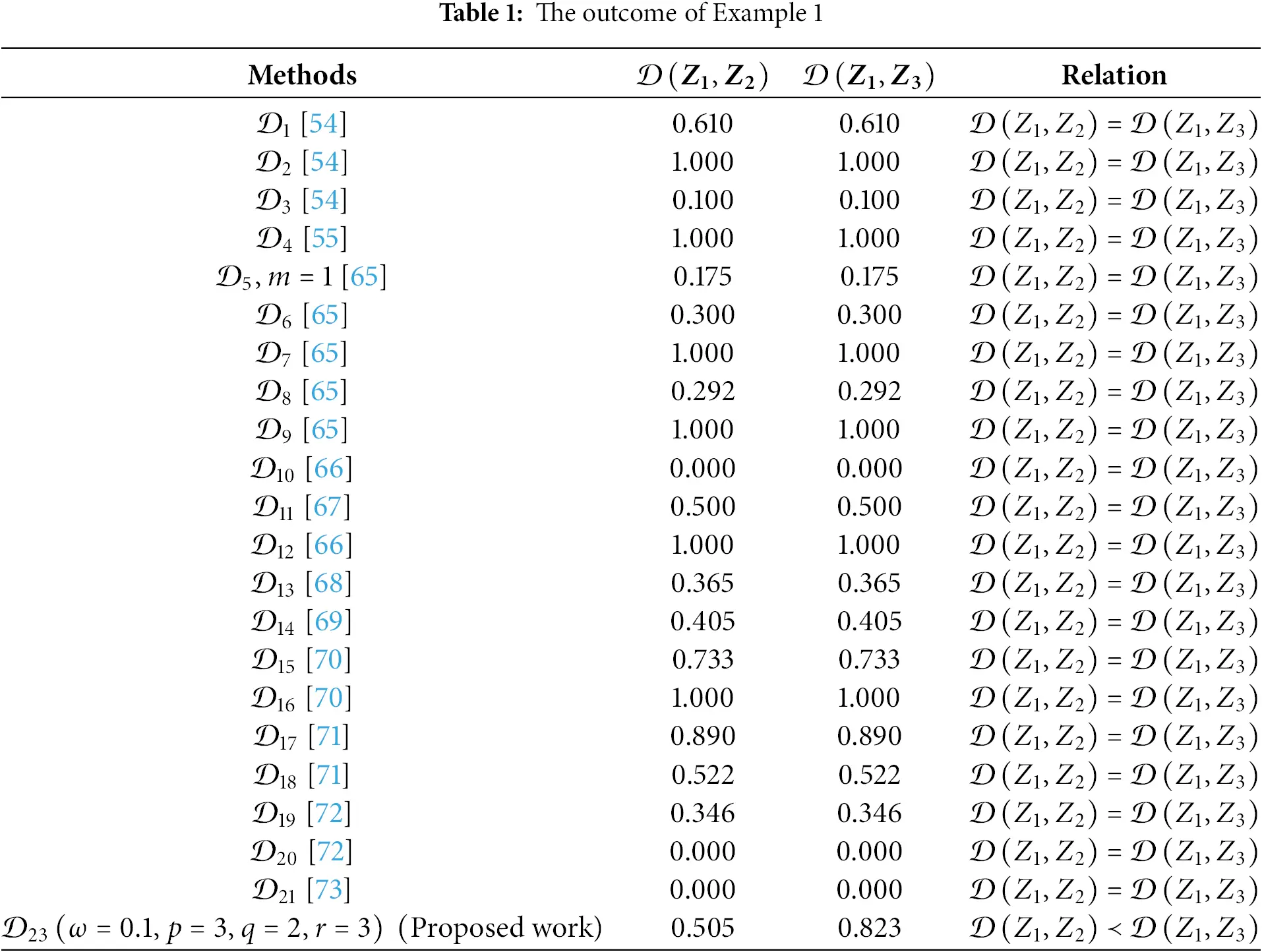
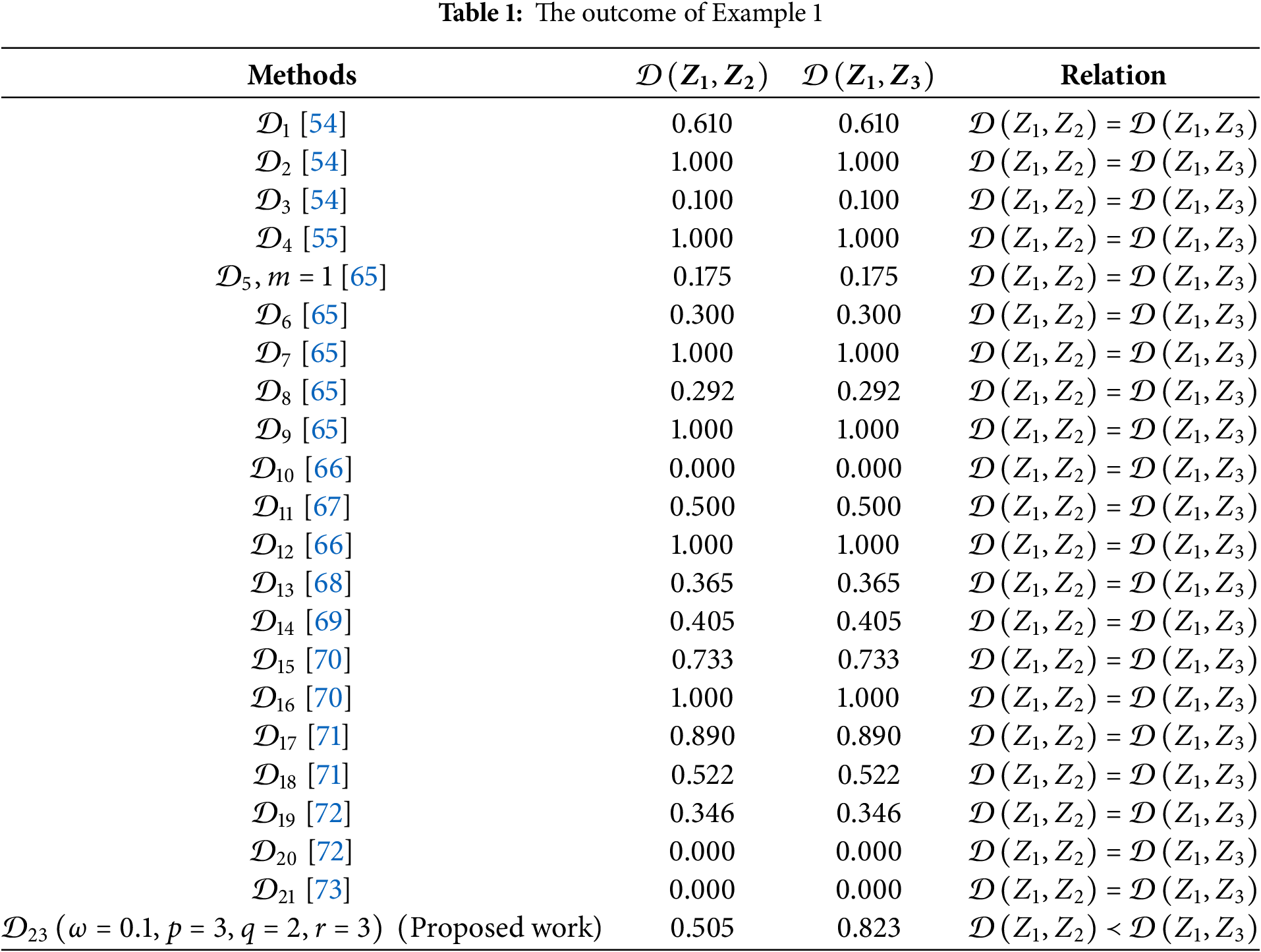
Example 1: Let us consider the p,q,r−spherical fuzzy numbers (p,q,r–SFNs) Z1, Z2, and Z3, defined over set G, where Z1=(1.0,0.0,0.0), Z2=(0.0,0.7,0.0), Z3=(0.0,0.0,0.7). A comparison of the distances between Z1 and Z2, as well as Z1 and Z3, is presented in Table 1 using the proposed DM alongside several existing methods. The analysis highlights significant shortcomings in certain existing DMs, including 𝒟1, 𝒟2, 𝒟3, 𝒟4, 𝒟5, 𝒟6, 𝒟7, 𝒟8, 𝒟9, 𝒟10 and 𝒟11. These measures rely on basic mathematical operations, such as addition, subtraction, maximum, or minimum, and fail to consider the intricate relationship between the positive, neutral, and negative membership degrees within the p,q,r–SF context. Other measures, such as 𝒟12, 𝒟13, 𝒟14, 𝒟15, 𝒟16, 𝒟17, 𝒟18 and 𝒟19, also yield inconsistent results due to the loss of critical information during their computation. The proposed distance measure addresses these issues by incorporating a more robust approach that preserves the underlying information structure. Although varying the parameter ω influences the calculated distance values, it does not affect the relative ranking of the alternatives. For instance, in a hypothetical thousand-person voting scenario, Z1=(1.0,0.0,0.0) represents a unanimous vote in favor, Z2=(0.0,0.7,0.0) reflects 700 neutral votes, and Z3=(0.0,0.0,0.7) indicates 700 votes against. Automatically, this suggests that Z2 is closer to Z1 than Z3, aligning with the proposed distance’s results where 𝒟(Z1,Z2)≼𝒟(Z1,Z2). In conclusion, the proposed distance measure overcomes the limitations of prior methods, offering a more reliable and intuitive approach to comparing picture fuzzy sets while maintaining critical information integrity.
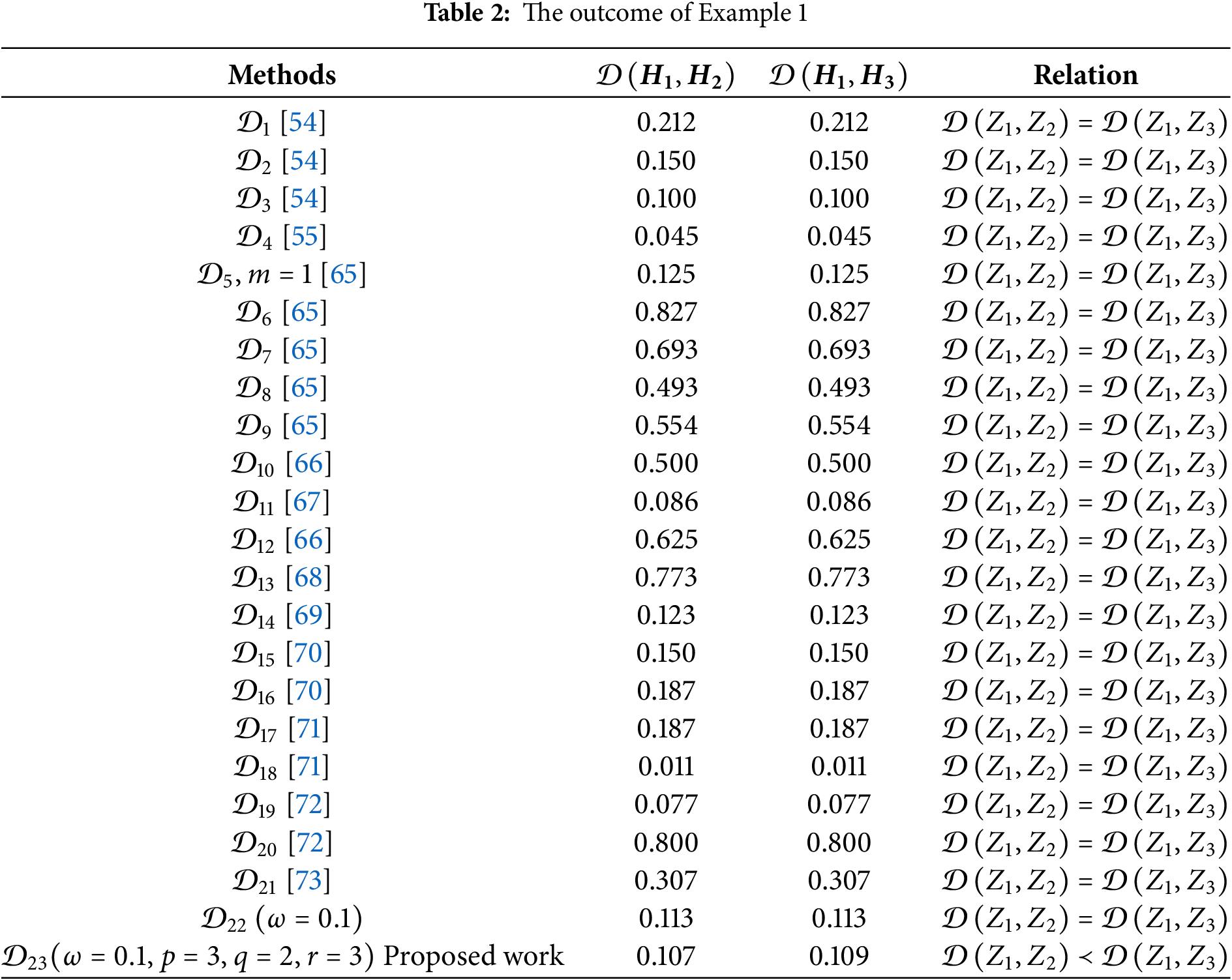
Example 2: Let us examine the Picture Fuzzy Sets (PFSs) A A, B B, and C C, defined on G={g1,g2}, where Z1={(0.30,0.20,0.40),(0.60,0.20,0.10)}, Z2={(0.30,0.10,0.40),(0.60,0.10,0.20)} and Z3={(0.20,0.20,0.40),(0.50,0.20,0.20)}.
Based on both scoring and intuitive reasoning, Z2 is evidently closer to Z1 than Z3, meaning that in terms of distance, 𝒟(Z1,Z2)≺𝒟(Z1,Z3). Table 2 presents a comparison of the distances between Z1 and Z2 and between Z1 and Z3, calculated using the proposed distance measure and various existing methods. Upon analyzing Table 2, it becomes clear that many existing distance measures erroneously suggest that Z1 has equal similarity to both Z2 and Z3, which contradicts intuitive reasoning. In contrast, the results produced by the proposed distance measure are consistent with human intuition, accurately reflecting the greater similarity between Z1 and Z2. This demonstrates the reliability and effectiveness of the proposed distance in capturing meaningful relationships between fuzzy picture sets.

Proposed MCDM Approach
In this subsection, we present an MCDM approach based on the proposed distance measures, considering m alternatives and nnn criteria. This approach extends the traditional AHP method to the p,q,r−spherical fuzzy environment for determining the unknown criteria weights.
Assume we have a set of alternatives Ξ={Ξ1,Ξ2,…,Ξm}, a set of criteria ζ={ζ1,ζ2,…,ζn}, and their weights are 𝓌={𝓌1,𝓌2,…,𝓌n}T associated with the criteria Cj such that 𝓌j∈[0,1] and ∑j=1m𝓌i=1. Consider a p,q,r−SF decision matrix denoted as V=(vij)mn(vij=(φij,ηij,ϑij)) represents the evaluation values of alternative Ξi with respect to criterion Cj. The φij, ηij and ϑij represents the MD, NEMD and NMD of alternative αj with respect to Ci and satisfy the conditions φij∈[0,1],ηij∈[0,1],ϑij∈[0,1], and φpij+ηrij+ϑqij≼1, where p and q are positive integers and r=max(p,q). A systematic approach to selecting the optimal alternative involves the following steps:
Step 1. Identify potential alternatives and their associated attributes in a decision-making problem, based on the opinions of decision-makers. Let Ξi denote the set of m alternatives, Cj (j=1,2,…,n) represent the set of n criteria.
V=((φ11,η11,ϑ11)(φ12,η12,ϑ12)(φ21,η21,ϑ21)(φ22,η22,ϑ22)⋯(φ1n,η1n,ϑ1n)(φ2n,η2n,ϑ2n)⋮⋱⋮(φ1m,η1m,ϑ1m)(φ2m,η2m,ϑ2m)⋯(φmn,ηmn,ϑmn))(35)
The decision matrix as presented in Eq. (35) is defined such that columns represent the evaluation criteria, and rows represent the various alternatives being evaluated in the decision-making problem.
Step 2. The cost (ψj) and benefit criteria (ψ~j) play a crucial role in decision making, as they enable the evaluation of alternatives based on their potential expenses and advantages. Cost criteria represent the negative consequences, while benefit criteria represent the positive outcomes. Normalization is essential to transform these criteria values into a common scale, allowing for comparability, avoidance of dominance, and improved accuracy. By normalizing cost and benefit criteria, decision-makers can ensure a fair and unbiased evaluation of alternatives, leading to more informed and effective decisions. In cases where the system involves both beneficial and non-beneficial (cost) criteria, normalization can be achieved using the following formula:
V~ij=(φij,ηij,ϑij)={(φij,ηij,ϑij),for 𝒞i∈ψ~j(ϑij,ηij,φij),for 𝒞i∈ψj(36)
Step 3. (Weights of criteria) The weights of the criteria in decision-making processes can be determined using various established methods, such as entropy, Interactive and Multicriteria Decision Making (TODIM), and the Analytic Hierarchy Process (AHP). Each of these techniques offers distinct advantages and faces inherent limitations depending on the nature of the decision-making problem and the type of data involved. For the proposed decision-making approach, we extend the traditional AHP method into the p,q,r–SF context, enabling it to handle higher levels of uncertainty and complexity associated with MCDM. This extension ensures a more robust and comprehensive weighting process, leveraging the unique properties of p,q,r–SFSs to model vagueness and ambiguity more effectively, ultimately enhancing the accuracy and reliability of the decision-making outcomes. The methodology is outlined in the following steps:
Phase 1. Generate a pairwise comparison matrix by translating expert panel inputs into linguistic terms, facilitating relative evaluation.
V~ij=(φij,ηij,ϑij)mn(37)
Phase 2. Utilize Eqs. (38) and (39) to calculate the differences matrix V~ij incorporating the lower and upper bounds of the MD, NEMD and NMD as follows:
ΨijL=φijLp−ηijUr−ϑijUq(38)
ΨijU=φijUp−ηijLr−ϑijLq(39)
Phase 3. Calculate the interval multiplicative matrix Ω=(Ωij)mn by applying Eqs. (40) and (41) as follows:
ΩijL=1000ΨL(40)
ΩijU=1000ΨU(41)
Phase 4. Determine the determinacy value λ=(λij)mn of dˇij by applying Eq. (42).
λij=1−(φijUp−φijLp)−ηijUr−ηijLr−ϑijUq−ϑijLq(42)
Phase 5. Calculate the pre-normalization weight matrix Ξ=(ζij)mn by multiplying the determinacy degrees with the matrix λ=(λij)mn, as given in Eq. (43).
ζij=(ΩijL+ΩijU+ΩijU3)×λij(43)
Phase 6. Determine the normalized priority weights, 𝓌i by applying Eq. (44).
wi=∑j=1mζij∑i=1m∑j=1mζij(44)
Step 4. Calculate the deviations of all alternatives from the optimal solution using the distance formula provided in Eq. (45).
𝒟𝓌(Ξij,Ξij)=13ln(1+1β)∑j=1m𝓌j(φZijp−φZijp×ln(β+φZijpβ+φZijp)+(φZijp+ηZijr−φZijp−ηZijr)×ln(β+φZijp+ηZijrβ+φZijp+ηZijr)+(ϑZijq−ϑZijq)×ln(1+β−ϑZijq1+β−ϑZijq))(45)
where β∈[0,1].
The extented AHP is employed to determine the weights of criteria within the proposed MCDM framework. The extension of traditional AHP into the (p,q,r)–SFS environment offers several advantages, in handling higher levels of uncertainty and imprecision. Unlike classical AHP, which relies on crisp pairwise comparisons, this extension incorporates spherical fuzzy membership functions, allowing decision-makers to express their preferences with more flexibility and accuracy. This is particularly beneficial in complex decision scenarios where subjective judgments are unavoidable. The rationality of this extension lies in its ability to model vagueness and ambiguity more effectively, ensuring that the assigned weights better reflect real-world uncertainties. Furthermore, the reasonability of the proposed approach is supported by its adherence to the fundamental principles of AHP while enhancing its applicability through divergence-based distance measures. These modification enables more robust and consistent weight calculations, leading to improved decision-making accuracy. By leveraging the strengths of (p,q,r)–SFSs, the extended AHP significantly enhances the reliability of ranking alternatives, making it a more suitable tool for modern MCDM problems.
4 Applications
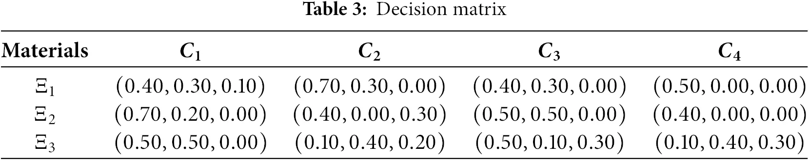
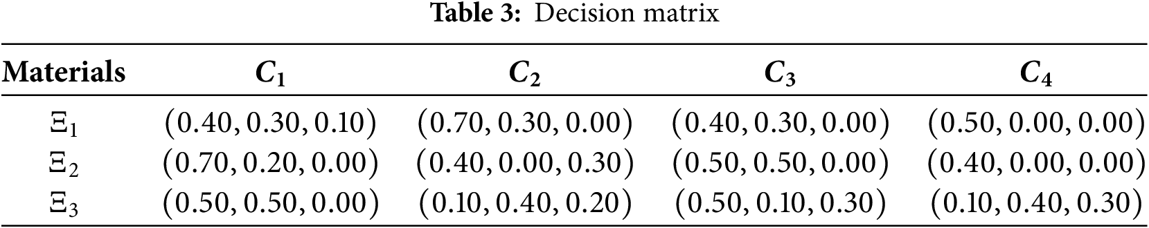
The quality of construction is fundamentally influenced by the quality of building materials used. Consequently, rigorous inspection of building materials serves as a cornerstone for achieving high engineering standards. Strict control during material selection is essential to ensure that only materials meeting the required specifications are utilized. Effective inspection practices enable builders to accurately distinguish between compliant and non-compliant materials, therefore enhancing the overall quality and durability of construction projects. To explore pattern recognition problems related to the classification of building materials, consider a scenario involving three distinct materials Ξ1, Ξ2 and Ξ3 represented in the set G={C1,C2,C3,C4} using p,q,r–SFSs. This approach highlights the critical role of advanced classification techniques in identifying and categorizing building materials to uphold construction quality standards.
Step 1. The information is summarized in Table 3.
Step 2. All criteria are treated as beneficial; therefore, normalization is not required.
Step 3. The extended AHP method is applied to determine the criteria weights, resulting in 𝓌1=0.5300, 𝓌2=0.1465, 𝓌3=0.2275, 𝓌4=0.0969.
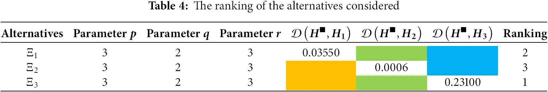
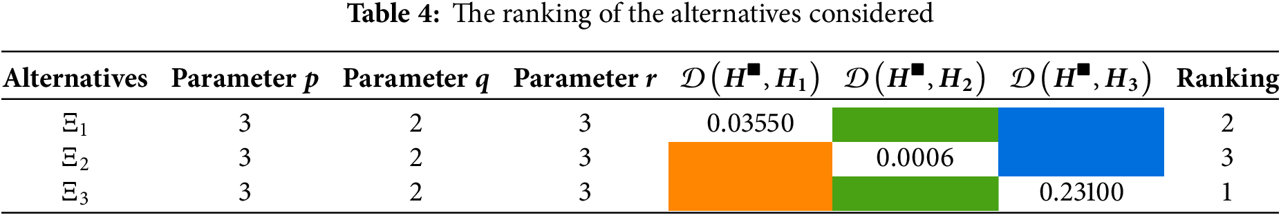
Step 4: The distances between ideal solution H◼=(0.70,0.00,0.00) of each alternative are calculated, where p=3, q=2, r=3, and ω=0.1. The ranking of alternatives is summarized in Table 4.
4.1 Influence of Parameter ω
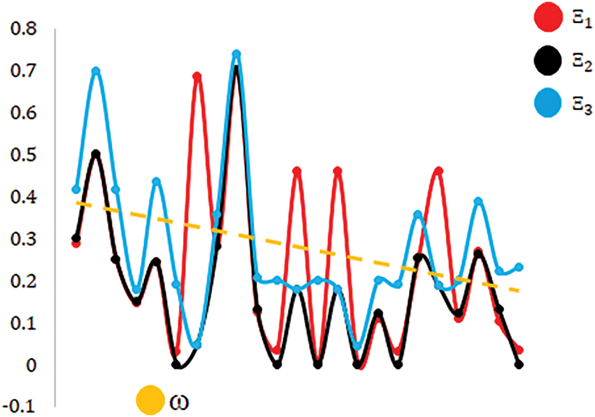
This section focuses on analyzing the behavior of three alternatives (Ξ1, Ξ2, and Ξ3), under the influence of a parameter ω. The figure provides a visual representation of how these alternatives vary with respect to changes in ω, emphasizing the oscillatory trends and the interaction of ω with each alternative. The objective is to explore the distinct patterns exhibited by Ξ1, Ξ2, and Ξ3, to compare their sensitivity to ω, and to evaluate the overall trend as influenced by the parameter ω. Such analysis identifies how different variables behave in dynamic systems where oscillatory changes and damping effects are critical. The impact of ω on the performance of the alternatives is depicted in Fig. 2.

Figure 2: The influence of parameter ω
The analysis of Ξ1, Ξ2, and Ξ3 under the influence of ω reveals distinct behavioral patterns and sensitivities. Ξ1 demonstrates pronounced oscillatory behavior, characterized by periodic peaks and troughs. However, as ω increases, the amplitude of these oscillations gradually decreases, indicating a damping effect. This suggests that Ξ1 is initially highly sensitive to variations in ω, but this sensitivity diminishes over time, reflecting a stabilizing influence. In contrast, Ξ2 exhibits a steady declining trend with relatively minor oscillations that are less pronounced compared to Ξ1. This behavior highlights Ξ1’s relative stability, indicating that it is less influenced by fluctuations in ω and follows a consistent pattern of reduction. Conversely, the blue curve Ξ3 maintains persistent and prominent oscillatory behavior, with no evidence of damping across the range of ω. This sustained oscillatory nature underscores Ξ1’s strong and continued sensitivity to ω, with periodic spikes suggesting reinforcement effects. The influence of ω, a downward-sloping trendline, reveals a general decline in its overall impact as ω increases. While ω exerts a noticeable damping effect on Ξ1 and Ξ2, it has minimal influence on the oscillatory behavior of Ξ3, suggesting that ω interacts differently with each function due to differences in their underlying structures.
4.2 Comparison with Existing Approaches
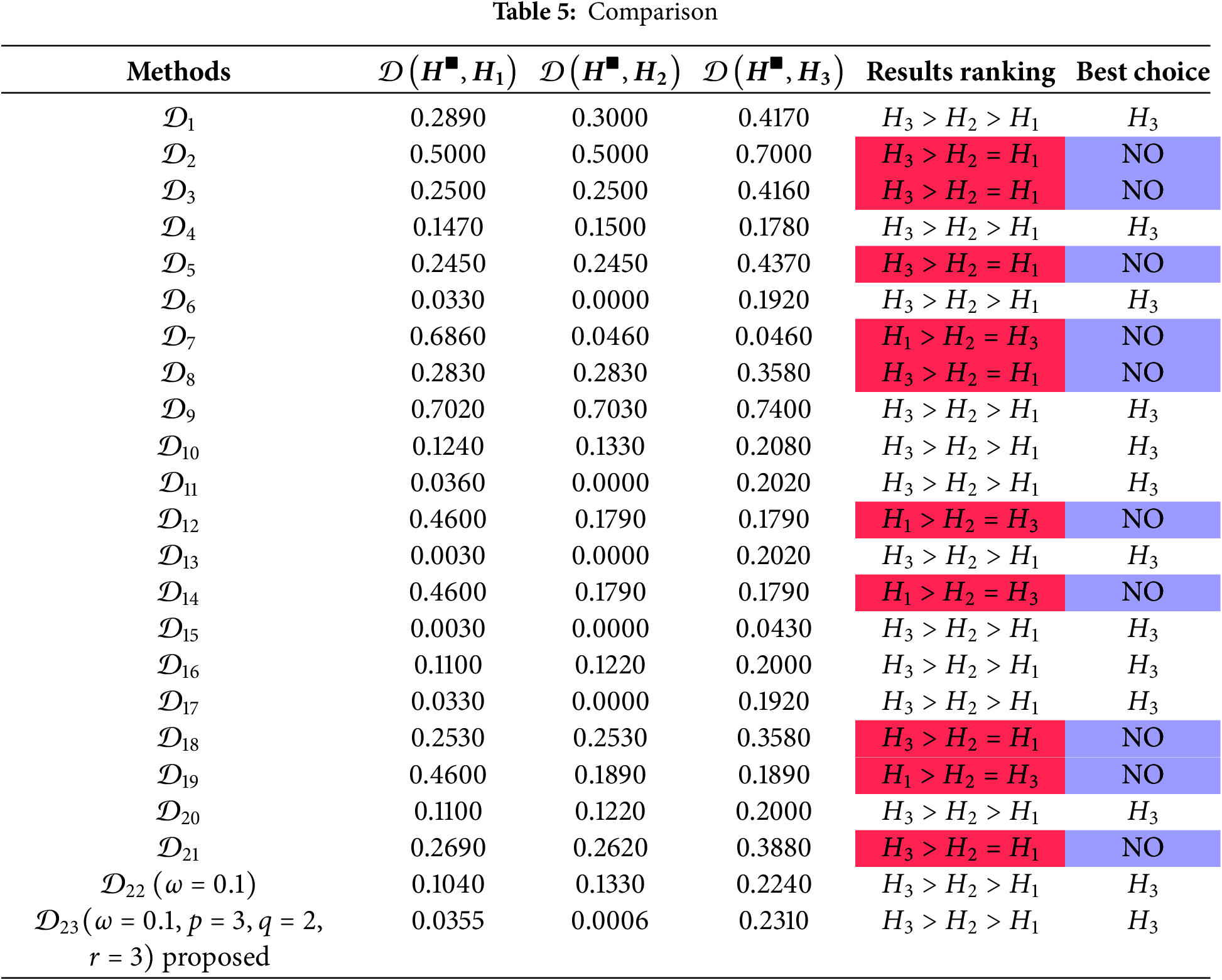
The effectiveness of the proposed approach is evaluated by comparing its results with those obtained using several existing methods to ensure its validity and reliability. For this purpose, the data presented in Table 3 is utilized, and the criteria weights are assigned as 𝓌1=0.5300, 𝓌2=0.1465, 𝓌3=0.2275, 𝓌4=0.0969, respectively. The comparative analysis of the final outcomes is summarized in Table 5. Upon examining the results in Table 5, it is evident that the proposed approach produces results consistent with those obtained by the majority of the existing approaches outlined in Definition 2. This alignment highlights the accuracy and robustness of the proposed method, demonstrating its capability to generate reliable decision-making outcomes that align with established methodologies. Such consistency further reinforces the practical applicability and scientific credibility of the proposed approach in addressing complex decision-making problems.
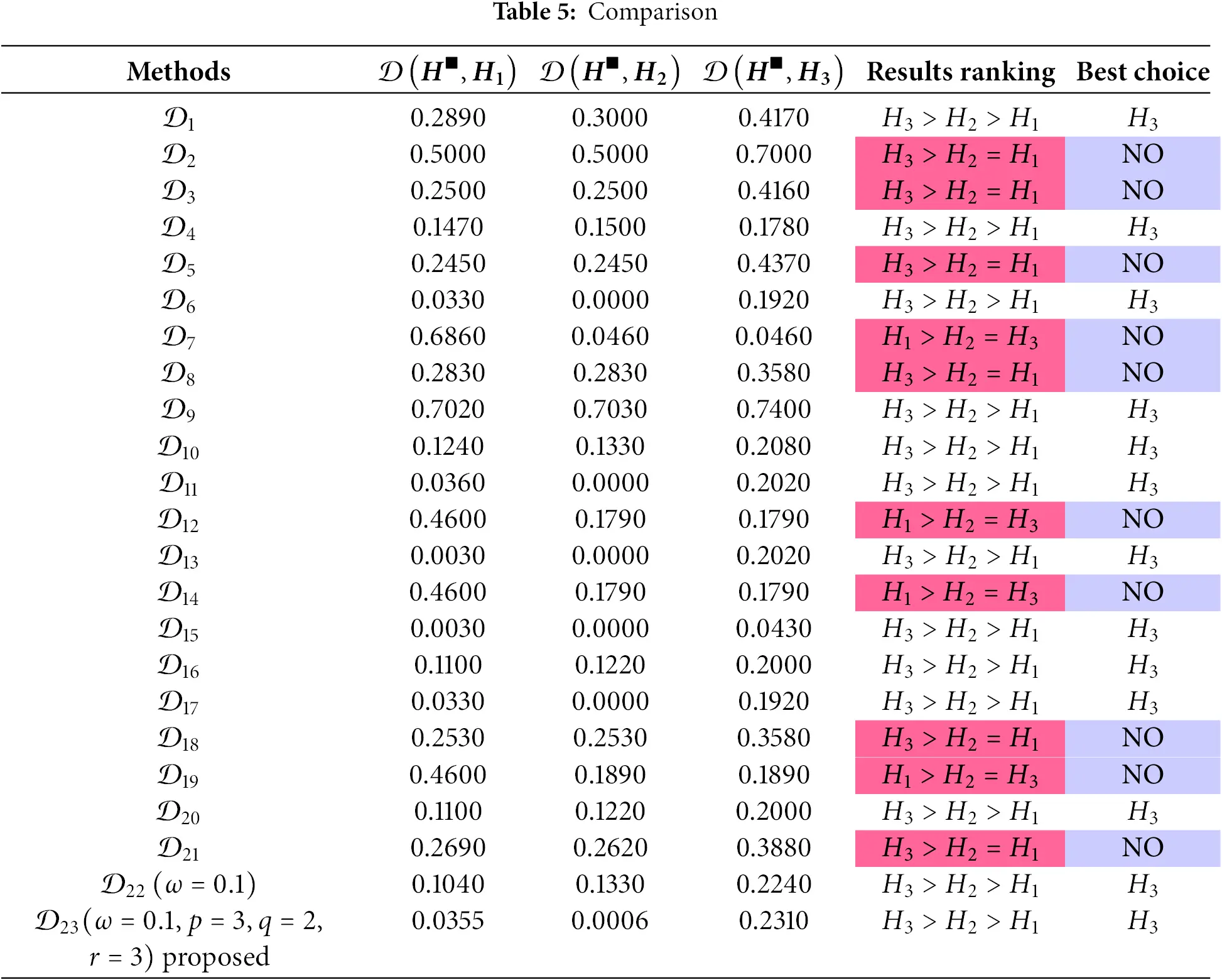
Table 5 presents comparative analysis of various distance measures 𝒟i (i=1,2,…,23) for evaluating alternatives Ξ1, Ξ2, and Ξ3, highlighting the effectiveness of the proposed measure. Most methods rank Ξ3≻Ξ2≻Ξ1, indicating a general consensus on Ξ3 as the best alternative. However, some methods exhibit ambiguity by ranking Ξ1=Ξ2, while others rank Ξ3>Ξ1=Ξ2, leading to inconsistent results. The proposed measure consistently produces the ranking Ξ3≻Ξ2≻Ξ1, with lower distances for Ξ1 and Ξ2 and a higher but distinguishable distance for Ξ3, ensuring clarity and robustness. Its advantages include improved sensitivity to small variations, a higher discrimination capability that avoids ambiguous rankings, and parameter integration (ω=0.1, p=3, q=2, r=3), which enhances adaptability and captures complex relationships. Additionally, the proposed measure aligns with logical expectations, providing intuitive and interpretable results while maintaining stability across scenarios, unlike some existing methods. These features make it a reliable tool for multi-criteria decision-making, offering better discrimination and consistent rankings, particularly in identifying Ξ3 as the best choice.
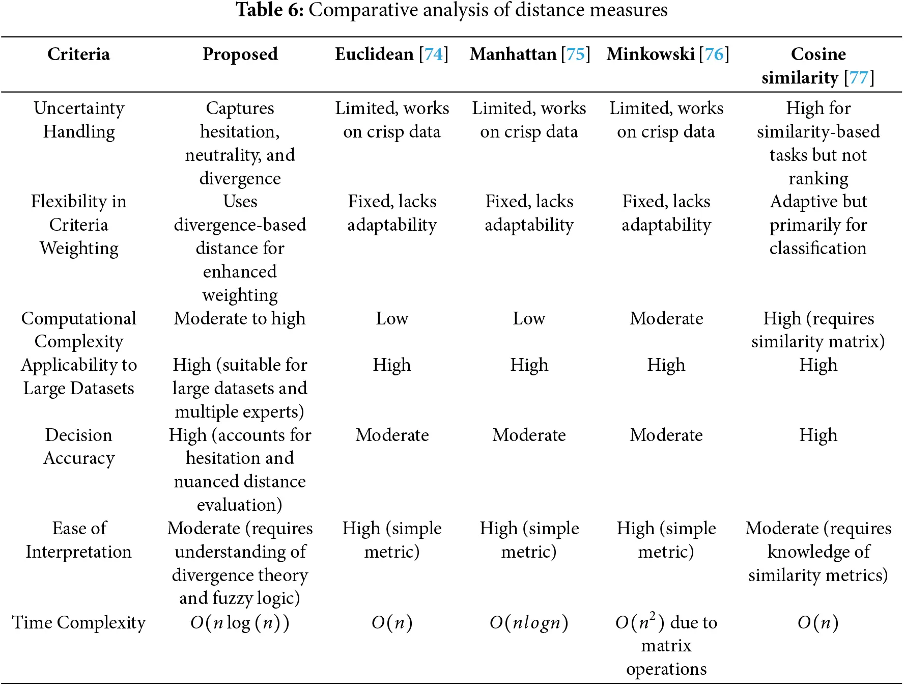
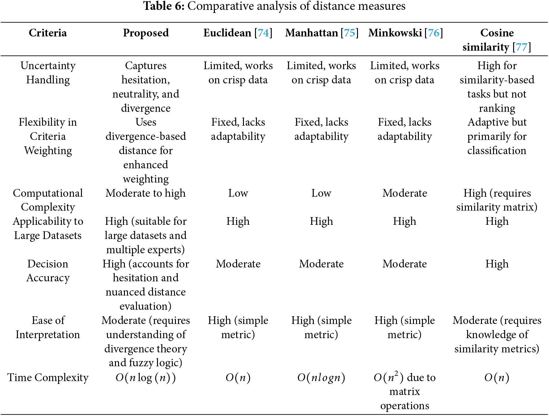
Table 6 evaluates the AHP-based divergence distance measure for (p,q,r)−SFSs against existing fuzzy distance measures based on uncertainty handling, flexibility in criteria weighting, computational complexity, applicability to large datasets, decision accuracy, ease of interpretation, and time complexity. Uncertainty handling reflects the ability to manage vagueness and hesitation in decision-making, where the proposed approach captures hesitation and neutrality better than conventional methods like Euclidean and Manhattan distances, which operate on crisp data. Flexibility in criteria weighting indicates how well a method adapts to different importance levels assigned to criteria, with divergence-based weighting offering greater adaptability compared to rigid approaches. Computational complexity measures the effort required to execute a method, where simple metrics like Euclidean distance have low complexity, while advanced techniques such as Hausdorff and Jensen-Shannon divergence require intensive calculations. Applicability to large datasets determines whether a method efficiently processes vast amounts of data, with the proposed approach proving highly effective in multi-expert and large-scale environments, unlike traditional AHP, which struggles with scalability. Decision accuracy assesses how precisely alternatives are ranked, with the divergence distance method improving ranking precision by incorporating hesitation factors, whereas conventional distance measures may yield ambiguous results. Ease of interpretation reflects how intuitively a method can be understood and implemented, with basic distance measures being simpler than fuzzy divergence-based approaches, which require knowledge of fuzzy logic and aggregation. Time complexity represented using Big O notation, describes how computational time grows with input size where O(nlog(n)) complexity in the proposed approach ensures efficiency for large datasets, contrasting with exponential-based methods that become computationally impractical. Big O notation provides insight into algorithm efficiency, helping to evaluate worst-case performance, where O(n) indicates linear time, O(nlog(n)) represents log-linear time, and O(n2) signifies quadratic time. The proposed divergence distance measure demonstrates strong performance across multiple criteria, making it a robust tool for multi-criteria decision-making while maintaining a reasonable computational cost.
The comparative analysis demonstrates that
1. The proposed divergence-based distance measure satisfies all axiomatic properties and provides better sensitivity to uncertainty variations in p,q,r–SFSs.
2. In MCDM applications, the proposed measure generates more consistent and stable rankings, reducing counter-intuitive outcomes observed in other distance measures.
3. The method achieves high computational efficiency, making it suitable for large-scale decision problems.
4.3 Advantages of the Proposed Work
The p, q, r–SFSs is the recent advancement of fuzzy set theory. This framework incorporating MD, NMD, and NEMD with the constraint 0≼φZp(g)+ηZr(g)+ϑZq(g)≼1 for all p,q, and r≽1 with r=max(p,q). This formulation enables more flexible and adaptive uncertainty modeling, allowing decision-makers to adjust the parameters p, q and r based on problem-specific needs. Unlike previous models, which impose rigid and symmetric relationships between membership and non-membership values, the proposed framework eliminates these constraints, thereby enabling a more comprehensive representation of real-world uncertainty. This flexibility makes p,q,r–SFSs particularly useful for multi-criteria decision-making (MCDM) problems involving uncertain, imprecise, and conflicting information. A key contribution of this work is the development of a divergence-based distance measure tailored for p,q,r–SFSs. Traditional distance measures, such as Hamming, Euclidean, and Hausdorff distances, often fail to maintain axiomatic properties such as non-negativity, symmetry, and triangle inequality, leading to counterintuitive results in decision analysis. The proposed divergence-based distance measure, as formulated in Eq. (28), satisfies fundamental axiomatic properties, including non-negativity, symmetry, and triangle inequality, ensuring logical consistency and reliability in decision analysis. This divergence-based measure significantly improves the differentiation capability among alternatives, ensuring mathematical consistency and resolving issues where previous distance measures yielded unreliable or undefined results. By leveraging divergence theory, the proposed measure not only quantifies the distance between fuzzy sets more accurately but also ensures greater robustness in decision-making applications, particularly in ranking alternatives under uncertainty. Furthermore, the proposed approach integrates the AHP within the p,q,r–SFS environment, providing a more refined mechanism for calculating criteria weights. Conventional AHP struggles with uncertainty due to its reliance on crisp pairwise comparisons, which limits its effectiveness in complex decision-making scenarios. By extending AHP into the p,q,r–spherical fuzzy domain, the proposed method enhances criteria weight computation, enabling a more rational, adaptive, and accurate decision-making process. The numerical validation demonstrates that this approach consistently outperforms existing methods, producing logically consistent and reliable results across different decision-making problems. These improvements make the proposed work a robust, mathematically grounded, and practically applicable tool for handling uncertainty in MCDM, significantly advancing the field of fuzzy decision analysis.
5 Conclusion
For existing FSs, the use of several distance measurements has not prevented the occurrence of unexpected outcomes. Upon closer examination of these distances, two primary causes for these unusual findings are revealed. Initially, the choice of distance metric can have a big impact on how similarity across sets is interpreted, which could result in results that are not intuitively expected. The complex structure of picture fuzzy sets, which include different levels of membership, neutral membership, and non-membership grades, can also make the analysis more difficult and lead to unanticipated connections between the data. We introduce a novel divergence-based distance metric between (p,q,r)–SFSs that satisfies the fundamental conditions. The proposed distance not only produces sensible results but also shows a high degree of confidence, according to case studies in multi-attribute decision-making.
Every research has its limitations, which future studies can address, and this study is no exception. Below are some of the limitations of the proposed work.
(1) Practical Implementation: High computational complexity in real-world scenarios with large datasets or multiple criteria.
(2) Parameter Sensitivity: Results are highly sensitive to the choice of parameters p, q, and r, affecting stability.
(3) Extreme Case Handling: May struggle with extreme membership values, leading to less accurate or impractical decisions.
(4) Generalizability: Limited applicability to other fuzzy set models, requiring adjustments for broader use.
Future research can explore the integration of additional decision-making criteria and alternative aggregation operators within the framework of p,q–quasirung orthopair fuzzy sets to enhance the robustness of the model. Additionally, the impact of varying parameters such as p, q, and r on decision outcomes can be further investigated, and real-world applications in different domains, such as healthcare and environmental sustainability, could be explored to validate the model’s effectiveness. Furthermore, the incorporation of machine learning techniques for automatic parameter tuning and expert weight determination could improve the accuracy and efficiency of decision-making processes.
Acknowledgement: The researchers would like to thank the Deanship of the Graduate Studies and Scientific Research at Qassim University for financial support (QU-APC-2025).
Funding Statement: The authors received no specific funding for this study.
Author Contributions: Shah Zeb Khan and Muhammad Rahim: Conceptualization; Methodology; Writing—original draft. A. Almutairi and Muhammad Rahim: Data curation; Formal analysis. Adel M. Widyan: Funding acquisition; Investigation; Project administration; Resources software. Njood Shaher Ethaar Almutire and Hamiden Abd El-Wahed Khalifa: Validation; Visualization; Supervision. All authors reviewed the results and approved the final version of the manuscript.
Availability of Data and Materials: All data generated or analyzed during this study are included in this published article.
Ethics Approval: Not applicable.
Conflicts of Interest: The authors declare no conflicts of interest to report regarding the present study.
References
1. Zadeh LA. Fuzzy sets. Inf Control. 1965;8(3):338–53. doi:10.1016/S0019-9958(65)90241-X. [Google Scholar] [CrossRef]
2. Demir G, Riaz M, Deveci M. Wind farm site selection using geographic information system and fuzzy decision making model. Expert Syst Appl. 2024;255(5):124772. doi:10.1016/j.eswa.2024.124772. [Google Scholar] [CrossRef]
3. Liu Y, Zhu L, Rodríguez RM, Martínez L. Personalized fuzzy semantic model of PHFLTS: application to linguistic group decision making. Inf Fusion. 2024;103(4):102118. doi:10.1016/j.inffus.2023.102118. [Google Scholar] [CrossRef]
4. Bani-Doumi M, Serrano-Guerrero J, Chiclana F, Romero FP, Olivas JA. A picture fuzzy set multi criteria decision-making approach to customize hospital recommendations based on patient feedback. Appl Soft Comput. 2024;153(2):111331. doi:10.1016/j.asoc.2024.111331. [Google Scholar] [CrossRef]
5. de Resende BA, Dedini FG, Eckert JJ, Sigahi TFAC, de Pinto JS, Anholon R. Proposal of a facilitating methodology for fuzzy FMEA implementation with application in process risk analysis in the aeronautical sector. Int J Qual Reliab Manag. 2024;41(4):1063–88. doi:10.1108/IJQRM-07-2023-0237. [Google Scholar] [CrossRef]
6. Rong Y, Yu L, Liu Y, Simic V, Pamucar D, Garg H. A novel failure mode and effect analysis model based on extended interval-valued q-rung orthopair fuzzy approach for risk analysis. Eng Appl Artif Intell. 2024;136(1):108892. doi:10.1016/j.engappai.2024.108892. [Google Scholar] [CrossRef]
7. Karanović V, Ceylan BO, Jocanović M. Reliable ships: a fuzzy FMEA based risk analysis on four-ram type hydraulic steering system. Ocean Eng. 2024;314(A1):119758. doi:10.1016/j.oceaneng.2024.119758. [Google Scholar] [CrossRef]
8. Sakr HH, Alanazi BS. Effective vague soft environment-based decision-making. AIMS Math. 2024;9(4):9556–86. doi:10.3934/math.2024467. [Google Scholar] [CrossRef]
9. Zhan J, Ye J, Ding W, Liu P. A novel three-way decision model based on utility theory in incomplete fuzzy decision systems. IEEE Trans Fuzzy Syst. 2022;30(7):2210–26. doi:10.1109/TFUZZ.2021.3078012. [Google Scholar] [CrossRef]
10. Alreshidi NA, Rahim M, Amin F, Alenazi A. Trapezoidal type-2 Pythagorean fuzzy TODIM approach for sensible decision-making with unknown weights in the presence of hesitancy. AIMS Math. 2023;8(12):30462–86. doi:10.3934/math.20231556. [Google Scholar] [CrossRef]
11. Atanassov KT. Intuitionistic fuzzy sets. Fuzzy Sets Syst. 1986;20(1):87–96. doi:10.1016/S0165-0114(86)80034-3. [Google Scholar] [CrossRef]
12. Lu XY, Dong JY, Wan SP, Li HC. Interactively iterative group decision-making method with interval-valued intuitionistic fuzzy preference relations based on a new additively consistent concept. Appl Soft Comput. 2024;152(8):111199. doi:10.1016/j.asoc.2023.111199. [Google Scholar] [CrossRef]
13. Wan SP, Dong JY, Chen SM. A novel intuitionistic fuzzy best-worst method for group decision making with intuitionistic fuzzy preference relations. Inf Sci. 2024;666(6):120404. doi:10.1016/j.ins.2024.120404. [Google Scholar] [CrossRef]
14. Yager RR. Pythagorean fuzzy subsets. In: 2013 Joint IFSA World Congress and NAFIPS Annual Meeting (IFSA/NAFIPS); 2013 Jun 24–28; Edmonton, AB, Canada. p. 57–61. doi:10.1109/IFSA-NAFIPS.2013.6608375. [Google Scholar] [CrossRef]
15. Peng X, Yang Y. Some results for Pythagorean fuzzy sets. Int J Intell Syst. 2015;30(11):1133–60. doi:10.1002/int.21738. [Google Scholar] [CrossRef]
16. Senapati T, Yager RR. Fermatean fuzzy sets. J Ambient Intell Humaniz Comput. 2020;11(2):663–74. doi:10.1007/s12652-019-01377-0. [Google Scholar] [CrossRef]
17. Yager RR. Generalized orthopair fuzzy sets. IEEE Trans Fuzzy Syst. 2017;25(5):1222–30. doi:10.1109/TFUZZ.2016.2604005. [Google Scholar] [CrossRef]
18. Seikh MR, Mandal U. Multiple attribute group decision making based on quasirung orthopair fuzzy sets: application to electric vehicle charging station site selection problem. Eng Appl Artif Intell. 2022;115(4):105299. doi:10.1016/j.engappai.2022.105299. [Google Scholar] [CrossRef]
19. Alreshidi NA, Shah Z, Khan MJ. Similarity and entropy measures for circular intuitionistic fuzzy sets. Eng Appl Artif Intell. 2024;131(10):107786. doi:10.1016/j.engappai.2023.107786. [Google Scholar] [CrossRef]
20. Uluçay V, Şahin M. Intuitionistic fuzzy soft expert graphs with application. Uncertain Discourse Appl. 2024;1(1):1–10. [Google Scholar]
21. Alkan N, Kahraman C. CODAS extension using novel decomposed Pythagorean fuzzy sets: strategy selection for IOT based sustainable supply chain system. Expert Syst Appl. 2024;237(4):121534. doi:10.1016/j.eswa.2023.121534. [Google Scholar] [CrossRef]
22. Akram M, Zahid S, Deveci M. Enhanced CRITIC-REGIME method for decision making based on Pythagorean fuzzy rough number. Expert Syst Appl. 2024;238(24):122014. doi:10.1016/j.eswa.2023.122014. [Google Scholar] [CrossRef]
23. Rahim M, Amin F, Shah K, Abdeljawad T, Ahmad S. Some distance measures for Pythagorean cubic fuzzy sets: application selection in optimal treatment for depression and anxiety. MethodsX. 2024;12(6):102678. doi:10.1016/j.mex.2024.102678. [Google Scholar] [PubMed] [CrossRef]
24. Khan M, Chao W, Rahim M, Amin F. Enhancing green supplier selection: a nonlinear programming method with TOPSIS in cubic Pythagorean fuzzy contexts. PLoS One. 2024;19(12):e0310956. doi:10.1371/journal.pone.0310956. [Google Scholar] [PubMed] [CrossRef]
25. Göçer F. A novel extension of fermatean fuzzy sets into group decision making: a study for prioritization of renewable energy technologies. Arab J Sci Eng. 2024;49(3):4209–28. doi:10.1007/s13369-023-08307-5. [Google Scholar] [CrossRef]
26. Ejegwa PA, Wanzenke TD, Ogwuche IO, Anum MT, Isife KI. A robust correlation coefficient for fermatean fuzzy sets based on Spearman’s correlation measure with application to clustering and selection process. J Appl Math Comput. 2024;70(2):1747–70. doi:10.1007/s12190-024-02019-1. [Google Scholar] [CrossRef]
27. Zheng Y, Qin H, Ma X. A novel group decision making method based on CoCoSo and interval-valued Q-rung orthopair fuzzy sets. Sci Rep. 2024;14(1):6562. doi:10.1038/s41598-024-56922-5. [Google Scholar] [PubMed] [CrossRef]
28. Ali Z, Yang MS. On circular q-Rung orthopair fuzzy sets with dombi aggregation operators and application to symmetry analysis in artificial intelligence. Symmetry. 2024;16(3):260. doi:10.3390/sym16030260. [Google Scholar] [CrossRef]
29. Rahim M, Eldin EMT, Khan S, Ghamry NA, Alanzi AM, Khalifa HAE. Multi-criteria group decision-making based on dombi aggregation operators under p, q-quasirung orthopair fuzzy sets. J Intell Fuzzy Syst. 2024;46(1):53–74. doi:10.3233/JIFS-233327. [Google Scholar] [CrossRef]
30. Zhao Z, Ye J, Rahim M, Amin F, Ahmad S, Asim M, et al. Quasirung orthopair fuzzy linguistic sets and their application to multi criteria decision making. Sci Rep. 2024;14(1):25513. doi:10.1038/s41598-024-76112-7. [Google Scholar] [PubMed] [CrossRef]
31. Cuong BC, Kreinovich V. Picture fuzzy sets. J Comput Sci Cybern. 2014;30(4):409–20. [Google Scholar]
32. Gündoğdu FK, Kahraman C. Spherical fuzzy sets and spherical fuzzy TOPSIS method. J Intell Fuzzy Syst. 2019;36(1):337–52. doi:10.3233/JIFS-181401. [Google Scholar] [CrossRef]
33. Ullah K, Mahmood T, Jan N. Similarity measures for T-spherical fuzzy sets with applications in pattern recognition. Symmetry. 2018;10(6):193. doi:10.3390/sym10060193. [Google Scholar] [CrossRef]
34. Rahim M, Amin F, Tag Eldin EM, Khalifa HW, Ahmad S. p, q-Spherical fuzzy sets and their aggregation operators with application to third-party logistic provider selection. J Intell Fuzzy Syst. 2024;46(1):505–28. doi:10.3233/JIFS-235297. [Google Scholar] [CrossRef]
35. Rahim M, Bajri SA, Khan S, Alqahtani H, Khalifa HAE. Innovative multi-criteria group decision making with Interval-valued p, q, r-spherical fuzzy sets: a case study on optimal solar energy investment location. Int J Fuzzy Syst. 2025;8(3):338. doi:10.1007/s40815-024-01905-x. [Google Scholar] [CrossRef]
36. Rahim M, Ahmad S, Bajri SA, Alharbi R, Khalifa HAE. Confidence levels-based p, q, r-spherical fuzzy aggregation operators and their application in selection of solar panels. IEEE Access. 2024;12:57863–78. doi:10.1109/ACCESS.2024.3389296. [Google Scholar] [CrossRef]
37. Dounis A, Palaiothodoros I, Panagiotou A. Medical diagnosis based on multi-attribute group decision-making using extension fuzzy sets, aggregation operators and basic uncertainty information granule. Comput Model Eng Sci. 2025;142(1):759–811. doi:10.32604/cmes.2024.057888. [Google Scholar] [CrossRef]
38. Ullah K. Picture fuzzy maclaurin symmetric mean operators and their applications in solving multiattribute decision-making problems. Math Probl Eng. 2021;2021(5):1098631–13. doi:10.1155/2021/1098631. [Google Scholar] [CrossRef]
39. Lei W, Ma W, Li X, Sun B. Three-way group decision based on regret theory under dual hesitant fuzzy environment: an application in water supply alternatives selection. Expert Syst Appl. 2024;237(1):121249. doi:10.1016/j.eswa.2023.121249. [Google Scholar] [CrossRef]
40. Deveci M, Raj Mishra A, Rani P, Gokasar I, Isik M, Delen D, et al. Evaluation of intelligent transportation system implementation alternatives in metaverse using a Fermatean fuzzy distance measure-based OCRA model. Inf Sci. 2024;657(3):120008. doi:10.1016/j.ins.2023.120008. [Google Scholar] [CrossRef]
41. Golui S, Mahapatra BS, Mahapatra GS. A new correlation-based measure on Fermatean fuzzy applied on multi-criteria decision making for electric vehicle selection. Expert Syst Appl. 2024;237(7):121605. doi:10.1016/j.eswa.2023.121605. [Google Scholar] [CrossRef]
42. de Keyser S, Gijbels I. Hierarchical variable clustering via Copula-based divergence measures between random vectors. Int J Approx Reason. 2024;165(1):109090. doi:10.1016/j.ijar.2023.109090. [Google Scholar] [CrossRef]
43. Liu Z. A distance measure of fermatean fuzzy sets based on triangular divergence and its application in medical diagnosis. J Oper Intell. 2024;2(1):167–78. doi:10.31181/jopi21202415. [Google Scholar] [CrossRef]
44. Patel A, Jana S, Mahanta J. Construction of similarity measure for intuitionistic fuzzy sets and its application in face recognition and software quality evaluation. Expert Syst Appl. 2024;237(3):121491. doi:10.1016/j.eswa.2023.121491. [Google Scholar] [CrossRef]
45. Kirişci M. New cosine similarity and distance measures for Fermatean fuzzy sets and TOPSIS approach. Knowl Inf Syst. 2023;65(2):855–68. doi:10.1007/s10115-022-01776-4. [Google Scholar] [PubMed] [CrossRef]
46. Gao P, Chen M, Zhou Y, Zhou L. An approach to linguistic q-rung orthopair fuzzy multi-attribute decision making with LINMAP based on Manhattan distance measure. J Intell Fuzzy Syst. 2023;45(1):1341–55. doi:10.3233/JIFS-221750. [Google Scholar] [CrossRef]
47. Ali J, Bashir Z, Rashid T. A cubic q-rung orthopair fuzzy TODIM method based on Minkowski-type distance measures and entropy weight. Soft Comput. 2023;27(20):15199–223. doi:10.1007/s00500-023-08552-8. [Google Scholar] [CrossRef]
48. Kamacı H. Complex linear Diophantine fuzzy sets and their cosine similarity measures with applications. Complex Intell Syst. 2022;8(2):1281–305. doi:10.1007/s40747-021-00573-w. [Google Scholar] [CrossRef]
49. Hussain Z, Alam S, Hussain R, ur Rahman S. New similarity measure of Pythagorean fuzzy sets based on the Jaccard index with its application to clustering. Ain Shams Eng J. 2024;15(1):102294. doi:10.1016/j.asej.2023.102294. [Google Scholar] [CrossRef]
50. Bhuyan HK, Chakraborty DC, Pani SK, Ravi V. Feature and subfeature selection for classification using correlation coefficient and fuzzy model. IEEE Trans Eng Manage. 2023;70(5):1655–69. doi:10.1109/TEM.2021.3065699. [Google Scholar] [CrossRef]
51. Shu X, Ye Y. Knowledge discovery: methods from data mining and machine learning. Soc Sci Res. 2023;110(1):102817. doi:10.1016/j.ssresearch.2022.102817. [Google Scholar] [PubMed] [CrossRef]
52. Elen A, Avuçlu E. Standardized variable distances: a distance-based machine learning method. Appl Soft Comput. 2021;98(2):106855. doi:10.1016/j.asoc.2020.106855. [Google Scholar] [CrossRef]
53. Pinar A, Boran FE. A novel distance measure on q-rung picture fuzzy sets and its application to decision making and classification problems. Artif Intell Rev. 2022;55(2):1317–50. doi:10.1007/s10462-021-09990-2. [Google Scholar] [CrossRef]
54. Van Dinh N, Thao NX. Some measures of picture fuzzy sets and their application. Issue Inf Commun Technol. 2017;3(2):35. doi:10.31130/jst.2017.49. [Google Scholar] [CrossRef]
55. Singh P, Mishra NK, Kumar M, Saxena S, Singh V. Risk analysis of flood disaster based on similarity measures in picture fuzzy environment. Afr Mat. 2018;29(7):1019–38. doi:10.1007/s13370-018-0597-x. [Google Scholar] [CrossRef]
56. Liu X. Entropy, distance measure and similarity measure of fuzzy sets and their relations. Fuzzy Sets Syst. 1992;52(3):305–18. doi:10.1016/0165-0114(92)90239-Z. [Google Scholar] [CrossRef]
57. Mahanta J, Panda S. A novel distance measure for intuitionistic fuzzy sets with diverse applications. Int J Intell Syst. 2021;36(2):615–27. doi:10.1002/int.22312. [Google Scholar] [CrossRef]
58. Xiao F. A distance measure for intuitionistic fuzzy sets and its application to pattern classification problems. IEEE Trans Syst Man Cybern Syst. 2021;51(6):3980–92. doi:10.1109/TSMC.2019.2958635. [Google Scholar] [CrossRef]
59. Liu Y, Jiang W. A new distance measure of interval-valued intuitionistic fuzzy sets and its application in decision making. Soft Comput. 2020;24(9):6987–7003. doi:10.1007/s00500-019-04332-5. [Google Scholar] [CrossRef]
60. Zhao R, Luo M, Li S. A dynamic distance measure of picture fuzzy sets and its application. Symmetry. 2021;13(3):436. doi:10.3390/sym13030436. [Google Scholar] [CrossRef]
61. Khan MJ, Kumam P, Deebani W, Kumam W, Shah Z. Distance and similarity measures for spherical fuzzy sets and their applications in selecting mega projects. Mathematics. 2020;8(4):519. doi:10.3390/math8040519. [Google Scholar] [CrossRef]
62. Wu MQ, Chen TY, Fan JP. Divergence measure of T-spherical fuzzy sets and its applications in pattern recognition. IEEE Access. 2019;8:10208–21. doi:10.1109/ACCESS.2019.2963260. [Google Scholar] [CrossRef]
63. Donyatalab Y, Gündoğdu FK, Farid F, Seyfi-Shishavan SA, Farrokhizadeh E, Kahraman C. Novel spherical fuzzy distance and similarity measures and their applications to medical diagnosis. Expert Syst Appl. 2022;191(8):116330. doi:10.1016/j.eswa.2021.116330. [Google Scholar] [CrossRef]
64. Karamaz F, Karaaslan F. Distance measures of r, s, t-spherical fuzzy sets and their applications in MCGDM based on TOPSIS. J Supercomput. 2024;81(1):173. doi:10.1007/s11227-024-06560-5. [Google Scholar] [CrossRef]
65. Wei G. Some cosine similarity measures for picture fuzzy sets and their applications to strategic decision making. Informatica. 2017;28(3):547–64. doi:10.15388/Informatica.2017.144. [Google Scholar] [CrossRef]
66. Luo M, Zhang Y, Fu L. A new similarity measure for picture fuzzy sets and its application to multi-attribute decision making. Informatica. 2021;2021(8):543–64. doi:10.15388/21-INFOR452. [Google Scholar] [CrossRef]
67. Wei G, Gao H. The generalized dice similarity measures for picture fuzzy sets and their applications. Informatica. 2018;29(1):107–24. doi:10.15388/Informatica.2018.160. [Google Scholar] [CrossRef]
68. Dutta P. Medical diagnosis via distance measures on picture fuzzy sets. Adv Model Anal A. 2017;54(2):657–72. [Google Scholar]
69. Khan MJ, Kumam P, Deebani W, Kumam W, Shah Z. Bi-parametric distance and similarity measures of picture fuzzy sets and their applications in medical diagnosis. Egypt Inform J. 2021;22(2):201–12. doi:10.1016/j.eij.2020.08.002. [Google Scholar] [CrossRef]
70. Singh S, Ganie AH. Applications of picture fuzzy similarity measures in pattern recognition, clustering, and MADM. Expert Syst Appl. 2021;168:114264. doi:10.1016/j.eswa.2020.114264. [Google Scholar] [CrossRef]
71. Verma R, Rohtagi B. Novel similarity measures between picture fuzzy sets and their applications to pattern recognition and medical diagnosis. Granul Comput. 2022;7(4):761–77. doi:10.1007/s41066-021-00294-y. [Google Scholar] [CrossRef]
72. Thao NX. Similarity measures of picture fuzzy sets based on entropy and their application in MCDM. Pattern Anal Appl. 2020;23(3):1203–13. doi:10.1007/s10044-019-00861-9. [Google Scholar] [CrossRef]
73. Luo M, Zhang G. Divergence-based distance for picture fuzzy sets and its application to multi-attribute decision-making. Soft Comput. 2024;28(1):253–69. doi:10.1007/s00500-023-09205-6. [Google Scholar] [CrossRef]
74. Moslem S, Pilla F. Addressing last-mile delivery challenges by using euclidean distance-based aggregation within spherical Fuzzy group decision-making. Transp Eng. 2023;14(9):100212. doi:10.1016/j.treng.2023.100212. [Google Scholar] [CrossRef]
75. Chiu WY, Yen GG, Juan TK. Minimum Manhattan distance approach to multiple criteria decision making in multiobjective optimization problems. IEEE Trans Evol Computat. 2016;20(6):972–85. doi:10.1109/TEVC.2016.2564158. [Google Scholar] [CrossRef]
76. Du WS. Minkowski-type distance measures for generalized orthopair fuzzy sets. Int J Intell Syst. 2018;33(4):802–17. doi:10.1002/int.21968. [Google Scholar] [CrossRef]
77. Rahim M, Amin F, Alhabeeb SA, Alshehri MH, Khalifa HAW. Cosine similarity and information measures of p, q, r-spherical fuzzy sets: application in selecting migration destination. Expert Syst Appl. 2025;265:125932. doi:10.1016/j.eswa.2024.125932. [Google Scholar] [CrossRef]

 Submit a Paper
 Propose a Special lssue
 Open Access
 View Full Text
 Download PDF
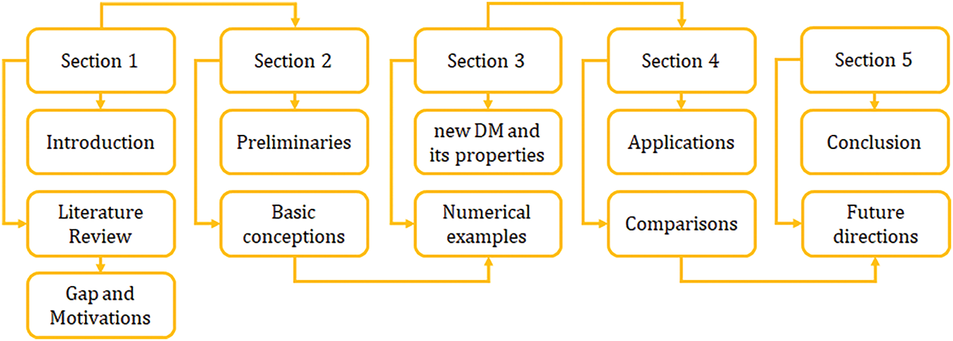
 Copyright © 2025 The Author(s). Published by Tech Science Press.
 Downloads
 Citation Tools