
 Submit a Paper
 Propose a Special lssue
 Open Access
ARTICLE

Non-Neural 3D Nasal Reconstruction: A Sparse Landmark Algorithmic Approach for Medical Applications
1 Institute of Intelligent and Interactive Technologies, University of Economics Ho Chi Minh City–UEH, Ho Chi Minh City, 70000, Vietnam
2 Anatomy Department, Pham Ngoc Thach University of Medicine, Ho Chi Minh City, 70000, Vietnam
* Corresponding Author: Nguyen Truong Thinh. Email:
(This article belongs to the Special Issue: Recent Advances in Signal Processing and Computer Vision)
Computer Modeling in Engineering & Sciences 2025, 143(2), 1273-1295. https://doi.org/10.32604/cmes.2025.064218
Received 08 February 2025; Accepted 16 May 2025; Issue published 30 May 2025
 View Full Text
 Download PDF
Abstract
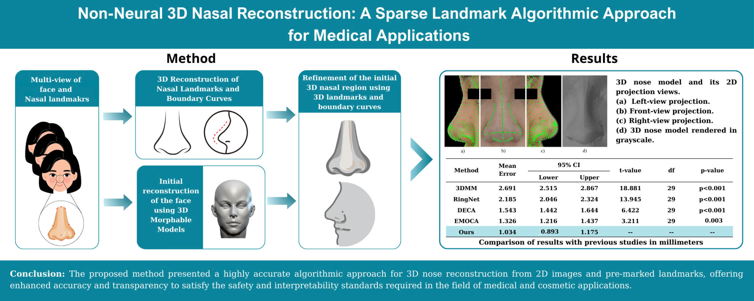
This paper presents a novel method for reconstructing a highly accurate 3D nose model of the human from 2D images and pre-marked landmarks based on algorithmic methods. The study focuses on the reconstruction of a 3D nose model tailored for applications in healthcare and cosmetic surgery. The approach leverages advanced image processing techniques, 3D Morphable Models (3DMM), and deformation techniques to overcome the limitations of deep learning models, particularly addressing the interpretability issues commonly encountered in medical applications. The proposed method estimates the 3D coordinates of landmark points using a 3D structure estimation algorithm. Sub-landmarks are extracted through image processing techniques and interpolation. The initial surface is generated using a 3DMM, though its accuracy remains limited. To enhance precision, deformation techniques are applied, utilizing the coordinates of 76 identified landmarks and sub-landmarks. The resulting 3D nose model is constructed based on algorithmic methods and pre-marked landmarks. Evaluation of the 3D model is conducted by comparing landmark distances and shape similarity with expert-determined ground truth on 30 Vietnamese volunteers aged 18 to 47, all of whom were either preparing for or required nasal surgery. Experimental results demonstrate a strong agreement between the reconstructed 3D model and the ground truth. The method achieved a mean landmark distance error of 0.631 mm and a shape error of 1.738 mm, demonstrating its potential for medical applications.Graphic Abstract
Keywords
The human face has a highly complicated structure with numerous delicate features, such as the shape of the nose, the contour of lips, and the curve of eyebrows. These elements contribute to the distinctive identity of each individual. While two-dimensional (2D) images are widely used across various applications due to their convenience and accessibility, they are inherently limited in their ability to capture the full spatial and depth information of the face. This limitation poses a significant challenge in scenarios requiring precise recognition and reconstruction of facial features, particularly in medical applications. Therefore, three-dimensional (3D) face reconstruction techniques have been increasingly developed. 3D face reconstruction refers to the creation of a three-dimensional model of the human face from two-dimensional sources such as images, depth maps, or scans. This technology involves accurately mapping facial features to produce shape, surface, and detail. Its applications span various fields, including medical treatment, cosmetic surgery, facial recognition, virtual reality, the creation of personalized prosthetics, and 3D interaction in medical education. Before the development of artificial intelligence (AI), 3D face reconstruction primarily relied on statistical model fitting methods or photometric methods. A key example is the 3D Morphable Model (3DMM) [1], a statistical model that captures variations in 3D facial shapes and textures. It enables 3D face reconstruction from 2D images by adjusting its parameters to match the input data. With advancements in deep learning (DL), modern approaches now leverage neural networks to predict 3D facial structures directly from 2D images. Notably, the research [2] proposes a dual-stream network for 3D face reconstruction from a single image, focusing on handling expression variations. These AI-driven techniques offer higher accuracy and better handling of variations in facial expressions, poses, and occlusions. However, 3D reconstruction models using neural networks face challenges in interpreting the results and are difficult to apply in the fields of medicine and cosmetic surgery.
The nose is an important part that performs many functions and is located in the center of the face. It is crucial for respiration and plays a role in pronunciation. The nose also contributes distinct characteristics for facial recognition. In aesthetics, it is a focal area of concern and impacts the way a person is perceived by the outside world [3]. In addition, its natural prominence makes it more prone to trauma, often requiring surgical intervention based on individual nose structure. However, research on 3D nose reconstruction has been limited due to the complexity of the nose compared to other facial regions such as eyes, and oral.
In the early stages, 3DMMs were used to reconstruct the entire face [4], including the construction of a 3D nose model. 3DMM is a widely applied method in the branch of statistical models in the field of 3D reconstruction from 2D images. This method is based on constructing a statistical model of facial shape and texture from a dataset of 3D scans. It allows the representation of any face as a linear combination of the faces in the learned dataset, thus creating a space of variability for both facial shape and texture. When inferred, the method can take one or more 2D images as input to reconstruct the corresponding 3D face. Thanks to its strong generalization ability, the model avoids generating unrealistic facial shapes. This advantage has made 3DMM a popular research direction. However, this method relies on Principal Component Analysis (PCA) [5], which introduces certain limitations in accuracy when evaluating complex regions, such as the nose.
To tackle the aforementioned problems, several hybrid methods have been explored. Notably, the study by Zhu et al. [6] proposed a 3D reconstruction and refinement process for the nose from a single image, based on a combination of the 3DMM model and coarse-to-fine correction. The process demonstrated outstanding results compared to previous methods, particularly in terms of personalization in 3D nose shapes. However, the procedure requires hardware for capturing RGB-D depth images. Additionally, the study does not include a corrective method for the radix point of the nose and nasal bridge area, which limits the ability to evaluate accuracy across the entire nose.
An alternative is the photometric method [7], which reconstructs an object’s 3D surface by analyzing multiple images captured under varying lighting conditions to deduce shape from light. The goal is to compute information about light direction and surface reflectance to reconstruct the 3D object. This method can accurately capture surface details such as wrinkles and skin texture, which statistical models like 3DMM are not able to achieve effectively. However, this approach is less commonly used for 3D nose reconstruction due to its strict requirements for control of lighting. These factors pose significant challenges when setting up systems in practical applications.
In recent years, deep learning methods have gained significant attention in the task of 3D face and nose reconstruction from 2D images. This approach differs from traditional techniques by its ability to directly learn the transformation from 2D images to 3D facial shapes, without relying on statistical or photometric models. Deep learning models can capture and process nonlinear transformations, enabling neural networks to learn complex representations of the face that linear models, such as 3DMM, are unable to achieve. As a result, they can offer higher accuracy compared to earlier approaches. However, one of the challenges in applying deep learning to 3D face reconstruction is the lack of real-world data. Unlike the previous methods, deep learning models require a significantly larger amount of data for training. Additionally, deep learning models face a critical issue known as the black-box problem. While neural networks can produce accurate results, the decision-making process of the model is often not easily interpretable. In sensitive fields like medical treatment or cosmetic surgery, safety and transparency are of paramount importance. These problems have led to practical challenges in the application of these models.
We propose a method for constructing a 3D of the nose from multiple 2D images to address the previously mentioned problems. This method focuses on improving the accuracy of the 3D nose model based on algorithmic methods and pre-marked landmarks without using deep learning techniques. This approach ensures the clarity, low computational cost, and applicability of the method in real-world medical problems and cosmetic surgery. The input consists of four 2D facial images with marked landmarks that include front, left, right, and bottom views. An estimated 3D structures algorithm is employed to generate the 3D coordinates of the landmarks based on their 2D positions from different perspectives. Camera parameters are also estimated during this process. The 3D landmarks are sparse and represent only the basic shape of the nose structure. Image processing techniques are applied then to identify the edges of the nose from 2D images and map them onto the 3D structure. Some unclear edges or lack information for precise coordinate determination are estimated through interpolation methods. Sub-landmarks are extracted from these edges to enhance the detail of the nose shape. At the end of this step, we have constructed 3D nose boundary curves with 17 landmarks and 45 sub-landmarks. Next, a combination of 3D Morphable Models and deformation techniques is used to generate the surface of the nose. The baseline nose surface is constructed using the 3DMM model. However, the accuracy of the surface is not high. Deformation is then applied to refine the nose surface in detail. The landmarks and sub-landmarks on the nose surface are identified as corresponding to points on the 3D nose boundary curves. The deformation technique modifies the positions of the landmarks and sub-landmarks on the surface to align with the corresponding points on 3D nose boundary curves while maintaining the reasonable shape of the nose. The final result is a highly accurate 3D nose model based on pure algorithms and pre-marked landmarks without the use of deep learning techniques.
The accuracy and reliability of the 3D nose model were evaluated using two distinct experiments. The first experiment compared the distance ratios between the landmark points of the 3D nose model and actual physical measurements. The second experiment assessed the discrepancies between the edges of the model and those manually defined by experts. The results demonstrate that the 3D nose model closely corresponds to real-world dimensions. In conclusion, the key contributions of this research can be summarized as follows:
• A novel method for constructing and refining a 3D nose model from four 2D images and predefined landmarks, particularly suitable for applications in healthcare and cosmetic surgery.
• A technique for generating boundary curves and sub-landmarks of the 3D nose model based on image processing algorithms.
• An approach to improving the accuracy of 3D models that does not rely on deep learning, making it more interpretable and safer for medical applications
Research on 3D face reconstruction from 2D images has achieved significant advancements. The 3D Morphable Model (3DMM) and its variants employ low-dimensional representations, which are widely used in practical applications. Research [6] enhances the reconstruction capability of 3DMM for occluded face image by incorporating pose-adaptive algorithms. The Basel Face Model (BFM) [7] is one of the most notable publicly available 3DMM models. BFM utilizes an improved registration algorithm, providing higher accuracy in both shape and texture. DL-3DMM [8] is another variant combining 3DMM and dictionary learning to enhance the reconstruction of facial expressions. However, these variants are all based on statistical foundations, making it challenging to capture detailed individual features. Recent studies have leveraged neural networks to enhance accuracy, resulting in impressive results. Specifically, a CNN architecture was used to regress 3DMM shape and texture parameters in research [9], improving accuracy. Subsequently, FGNet [10] also based on CNN to fine-grain the 3DMM model. In addition, researches [11,12] did not rely on the 3DMM but instead utilized GAN [13] to directly generate 3D faces. However, while these neural network methods provide good generalization in full face reconstruction, their results remain difficult to explain.
Several studies have applied sparse landmarks to refine 3D face models. Research [14] proposed an improved method to ensure the model performs well even when the face undergoes significant changes in expression, angle, and lighting conditions. The landmarks are used to align and optimize entire 3D model, including the nose. Results showed that the Mean Absolute Error (MAE) of this method was lower compared to previous deep learning-based methods. Recently, Ding and Mok [15] introduced a method to construct 3D facial models using deep learning and then refine them by automatically detecting sparse landmarks. However, using sparse landmarks leaves many regions of the 3D model unrefined. Notably, the lateral wall area of nose lacks sufficient sparse landmarks. To address this problem, Wood et al. [16] proposed increasing the number of landmarks from 68 to over 700 points that were detected by a CNN network. The authors then aligned a morphable 3D model based on these landmarks. In their paper, they also emphasized that a large number of accurate 2D landmarks and a 3D model are sufficient to reconstruct the face without requiring complex parametric models or algorithms. However, using CNNs to predict landmarks can result in unpredictable and inexplicable errors.
The aforementioned research primarily focuses on the reconstruction of entire face without specific attention to the refining and evaluation of local regions. Notably, local features of the eyes, nose, and mouth have not been fully represented. Compared to using sparse facial landmarks for the entire face, employing local landmarks for refining results better in local regions. The study by Wen et al. [17] introduced a system for real-time tracking and reconstruction of 3D eyelid shape and movement. A holistically-nested neural network (HNN) [18] was adapted to detect and classify the edges of eyes. These edges were then used to reconstruct and refine the 3D model of eyes. Another study by Wang et al. [19] presented a highly accurate real-time 3D gaze tracking method using an RGB camera. Landmarks around the eyes and segments of the iris were used to refine the 3D model, enhancing its adaptability to complex factors such as variations in lighting, head posture, and facial expressions.
For lip correction, the research of Garrido et al. [20] introduced a novel method aimed at enhancing the accuracy of 3D lip reconstruction from RGB video. The inner and outer contours of the lips were utilized to improve the accuracy of the regression model that was used for predicting the 3D shape of lips. Similarly, a regression-based approach for 3D lip reconstruction was also proposed in another research [21]. The author solved reconstruction error problems with user-guided assistance. More recently, factors influencing the quality of lip motion in 3D models were investigated in [22], with quantitative evaluation based on the Root Mean Square Error (RMSE).
Fewer studies focus on 3D nose reconstruction and refinement compared to other facial features, likely due to the complex geometry of nose. According to our survey, only one research of Tang et al. [23] aimed to correct a 3D nose model from 2D images. This research introduced a process for reconstruction from coarse to fine stages, starting with the reconstruction of a rough 3D model, which was then gradually refined based on 3D–2D curve correlation constraints. Sparse nose landmarks were automatically detected and used for coarse refining of the 3D model. Subsequently, depth information from RGB-D images was utilized for dense refining. The results demonstrated that the method excelled in reconstructing various nose shapes. However, the nose model did not include the radix point of nose and nasal bridge areas. In addition, the research required hardware setup to capture RGB-D images.
Deformation technique is widely applied in the problem of refining 3D models based on landmarks without abnormal distortions. The general idea is to adjust the position of vertices to better fit the landmarks on the face. The number and location of landmarks are defined differently depending on specific cases. For example, the 300-W dataset [24] defines 68 landmarks. Another dataset in the study [25] defines 35 landmarks. Laplacian deformation technique [26] is applied in researches [27] to refine the 3D model of the face with constraints from 2D landmarks while preserving local details. The research by Li et al. [28] utilizes this technique to refine 3D facial models in animated character creation. In [23], Laplacian deformation is also used to roughly refine the 3D nose shape during the Sparse Nose Correction stage. An alternative approach is As-Rigid-As-Possible (ARAP) Deformation [29], which focuses on preserving local rigidity. The study by Seylan and Sahillioğlu applies the ARAP method to 3D shape deformation based on stick figures [30]. However, the strict enforcement of local rigidity limits ARAP’s ability to smooth surfaces, making them appear stiff and unnatural. Research in [31] integrates ARAP and Laplacian Smoothing to enhance deformation quality in voxel-based human deformation modeling. Similarly, the study in [32] introduces a robust framework for mesh editing, combining ARAP and Laplacian Smoothing to improve the deformation process.
The proposed method constructs a 3D nose model using four 2D facial images from different angles and 21 predefined 2D landmarks, being key points manually marked on the face to guide reconstruction. The input images are taken with a monochromatic background to facilitate the application of image processing algorithms. Based on the 2D landmarks (LM2D), the Structure from Motion (SfM) algorithm is employed to determine the 3D spatial coordinates of landmarks (LM3D). Camera parameters are also estimated during this process. Simultaneously, the edges of nose in the 2D images are detected by combining edge detection algorithms, morphological operations. The 3D boundary curves of nose (B3D) are then reconstructed by aligning these edges into the 3D space defined by the landmarks. Subsequently, sub-landmark points are extracted from these boundary curves. At this stage, the total number of landmark and sub-landmark points, referred to as ad-landmarks (ad-LM), has been determined to be 76 points. A 3D Morphable Model (3DMM) is utilized to create a based-3D face model (MF) from the 2D images. Finally, ARAP deformation and Cotangent Laplacian Smoothing [33] utilizes ad-landmarks to refine the nose region of base 3D model. The entire pipeline is illustrated in Fig. 1.

Figure 1: Pipeline of proposed 3D nose reconstruction method
3.2 3D Landmark Reconstruction
The 2D RGB images utilized in this study consist of four facial images captured from different angles. The landmarks employed in this stage include a total of 21 points, of which 19 were synthesized from previous studies [34,35], and an additional 2 points called md were specifically defined by our team. The data is presented in Fig. 2. The origin point O is set at landmarks g, as shown in Fig. 2e. Due to the unavailability of camera parameters, the Structure from Motion (SfM) algorithm is employed to construct 3D landmarks and estimate camera parameters. The optimization equation for this process is illustrated below:

Figure 2: Input 2D images and landmark points. (a) bottom view (b) front view (c) left view (d) right view (e) landmarks on the nose
LMj3D represents the 3D coordinates of the j-th landmark. LMi2D,j denotes the 2D coordinates of j-th landmark in the i-th mage. Pi is the projection matrix of the i-th camera used to project 3D points onto 2D space. Each camera has unique parameters depending on its position, orientation, and intrinsic parameters. The term ||LMi2D,j − Pi LMj3D||2 can be interpreted as the L2 Loss between the observed 2D coordinates and the estimated coordinates obtained from the SfM algorithm. The result after optimization includes the 3D coordinates of the landmarks LMj3D as shown in Fig. 3, along with the projection matrices Pi of the cameras.

Figure 3: The 3D landmarks reconstructed in the first stage. (a) Frontal view showing red landmarks and blue wireframe. (b) Isometric view of the same 3D landmarks, providing a three-dimensional perspective
3.3 Boundary Curve Reconstruction
This stage presents a novel method that utilizes image processing techniques to identify the edges of the nose from 2D images. These edges are then mapped into a 3D space to construct boundary curves, aiming to enhance level of detail for boundaries in the nose model. Specifically, this section extracts six types of nose edges.
The mid-curve is a curve passing through a sequence of points g-n-k-r-prn-c-sn illustrated by the blue arrows in Fig. 4a. The background of the input image is set to a monochromatic color in the data collection process. This approach simplifies removal of the background. A thresholding algorithm is applied in the HSV color space. Each output pixel Iregb (xi, yi) is determined by the Eq. (2). The result was shown in Fig. 4b.

Figure 4: Sequential Process of mid-curve detection. (a) Original left-view image of the sample. (b) HSV thresholding result, isolating the facial region against the background. (c) Binary mask generated from the thresholded image. (d) Mid-curve extracted by identifying the first white pixel from left to right in the mask
Let Tthresh be the threshold selected based on the pre-configured background setup. The term (xi, yi) represents the pixel coordinates within the image, distinguishing them from (x, y, z) in the 3D space in Fig. 3. The image Irebg is converted into a mask (Fig. 4c), and the following equation is then applied to determine the mid-curve. Eq. (3) describes the set of pixel coordinates that create the mid-curve MC by identifying the first white pixel from left to right, where H is the height of image. The results are shown in Fig. 4d.
To map 2D points in MC onto the 3D model, the Closest Point Calculation method and interpolation techniques are employed. Fig. 5 illustrates this process, where M3D is the result of mapping from the point M2D (xi, yi) on the image into 3D space. According to the Structure from Motion algorithm, the point M3D lies on the green line of sight. However, information from the 2D image is insufficient to determine distance from the camera to M3D. The below algorithm is applied to determine the position based on the assumption that M3D is the intersection of the green line of sight and the blue line passing through the two nearest landmarks. The green line of sight is determined by constructing the line passing through points PC and M2D, where PC represents the coordinates of the camera in 3D space. The point M2D (xi, yi) in the 2D space of the i-th image must be transformed into a 3D spatial coordinate. There are two steps to transform. First, Eq. (4) is used to convert the coordinates of M2D from the 2D image coordinate system into the camera coordinate system. The homogeneous coordinate form M2D = [xi, yi, 1]T represents the coordinates of M2D. Here, K denotes the intrinsic matrix of camera, estimated during the SfM computation, as shown in Eq. (5). The parameters fx and fy are the focal lengths along the x and y axes in pixel units. cx and cy are the principal point coordinates on the image plane. Second, the rotation matrix R and the translation vector T are employed to transform MC2D into 3D coordinate system, as detailed in Eq. (6).

Figure 5: The process of mapping the point Mimg3D from 2D space to the point M3D in 3D space based on the relationship between already mapped landmark points
Two points, PC and Mimg3D, are utilized to define the green line of sight L1. Similarly, two points, LM13D and LM23D, are employed to establish the blue line L2. The specific coordinates of point M3D are determined as the intersection of lines L1 and L2. Both of these lines are derived using an estimation method, which inherently involves a certain degree of error. Consequently, in many cases, they do not actually intersect, making it impossible to directly find the intersection point.
To address this issue, the Closest Point Calculation method is employed. Assuming that the parametric equations of L1 and L2 are presented in Eq. (7), the point of intersection with the minimal deviation is identified by solving Eq. (8). The process involves expanding, simplifying, and deriving with respect to two variables t and s to obtain the system of equations in Eq. (9). Solving this system yields the optimal values t’ and s’ corresponding to two optimal points on each line. Finally, the coordinates of M3D are estimated as the midpoint of these two points, as presented in Eq. (10). This process is applied sequentially to consecutive point pairs in the sequence g-n-k-r-prn-c-sn. The result is a mid-curve 3D estimated from 2D images and landmark points.
The bottom-curve represents the contour of nose when viewed from bottom, extending from left to right and passing through the points ac-al-al′-add-prn-add-al′-al-ac. Seven of these points are landmarks previously introduced in Section 3.1. We define the addition of two purple-colored points called add to enhance edge detection. The coordinates of these points do not require high precision. They simply need to be approximately positioned between points al′ and prn along the nose edge when viewed from the bottom perspective. Fig. 6 shows where these points are located. Similar to the other landmarks, add points are manual marked.

Figure 6: Sequential process of detecting the nose bottom curve. (a) Bottom-view image of the sample. (b) Edge detection result. (c) Bottom-curve reconstructed by applying pathfinding algorithms
The Scharr gradient filter is applied to detect edges of the nose through landmarks on the bottom-curve using Eq. (11). Where K denotes the gradient magnitude at coordinate (xi, yi), while M represents the set of gradient magnitude values K(xi, yi) across the entire image. The terms Gxi, Gyi refer to the Scharr kernels in the xi and yi axis, respectively. The symbol * indicates the convolution operation. The result of the Scharr gradient filter is shown in Fig. 6b. However, some segments of the edge remain unclear due to high color similarity in the skin tone.
Pathfinding algorithms are applied to connect these unclear segments together with minimal cost. The optimization equation is presented in Eq. (12), where P represents the path connecting two consecutive landmarks, and C(ik, jk) denotes the movement cost between pixel points along the path. This cost is determined by the gray value at the pixel of destination point. The path P is illustrated as a green curve in Fig. 6c. In a similar manner to the mid-curve approach, the estimating intersection method of two lines is employed to transform 2D coordinates (xi, yi) into 3D coordinates (xBC, yBC, zBC).
3.3.3 Ala-Curve and C-Curve Extraction
The Ala-curve AC is defined as a curve passing through the ac-al-int landmarks composed of left and right parts, as shown in Fig. 7a. The C-curve CC follows a path md(left)-c-md(right), as displayed in Fig. 7b. Both curves are reconstructed using a method similar to the approach of the bottom-curve. By applying a combination of the Scharr gradient filter and pathfinding algorithms, the 2D curves are accurately identified. The mapping process from 2D coordinates to 3D coordinates is conducted similar to the mid-curve approach.

Figure 7: Results of detecting the Ala-curve and C-curve in 2D. (a) Left and right Ala-curve passing through landmarks ac-al-int. (b) C-curve passing through landmarks md(left)-c-md(right)
The nasal-sill NS includes two closed curves defining the borders of nostrils. Based on Fig. 8, a clear color contrast between the nostril area and its surroundings is observable. The Color Thresholding algorithm, as presented in Eq. (3), is used to identify the dark-colored areas considered as nostrils. This algorithm enables a relative detection of the nostril shape, though it still contains significant noise like black spots. The closing algorithm (13) in morphology is applied for noise reduction. Result is shown in Fig. 8b.

Figure 8: Sequential process of detecting nasal-sill. (a) Original bottom-view of the sample. (b) Result of color thresholding that isolates the nostril areas. (c) Nasal-sill after being extracted
The 2D nasal-sill was detected using the Contour Tracing Algorithm, following Eq. (14). Where A(xi, yi) represents the set of neighboring pixels for the pixel located at coordinates (xi, yi), while (xi ′, yi ′), represents the coordinates of a pixel within the neighboring set A(xi, yi). The nasal-sill only has information about passing through a single point al ″, which is insufficient to define its position in 3D space. Therefore, we assume that the nasal-sill has a normal vector perpendicular to the md-c line and parallel to the Oxy plane. The result of mapping NS into 3D space is shown in Fig. 9.
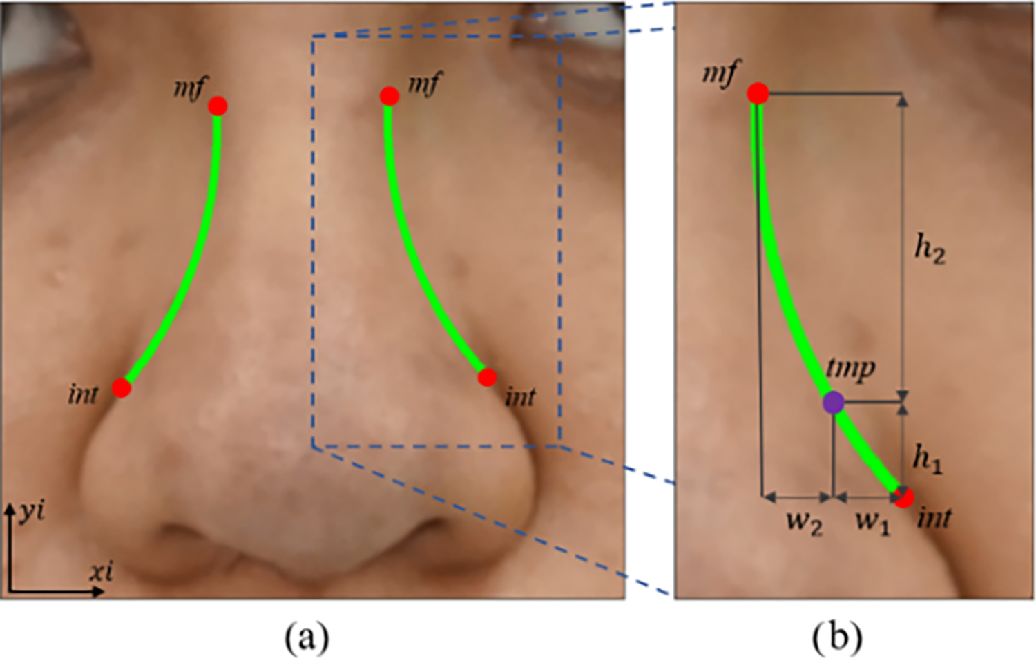
Figure 9: The results of side-curve detection. (a) Depict the two approximated int-mf curves (left and right) of the nose. (b) Detail the parameters used for the approximation, including the tmp point in purple, determined by the dimensions w1, w2, h1, and h2
The side-curve represents a curve passing through int-mf but lacks distinct features, making it hard to identify in 2D images. We propose a curve equation based on landmark coordinates. Specifically, the side-curve is approximated by a circle passing through the three points int, mf, and tmp. Where, the point tmp in purple is an additional point determined based on relative distance to landmark int using Eq. (15). In the other words, w1 = w2 and h2 = 3h1 as shown in Fig. 9b. The selection of these parameters is based on the steep change in y-values within segment w1 and the gradual change observed in segment w2. The circle passing through three points is determined by an Eq. (16) where the coefficients δ1, δ2, δ3 are defined in Eq. (17). The circular segment between int and mf is transformed into 3D space, similar to the Ala-curve. The results are shown in Fig. 9a.
The six curves in this section are extracted from 2D images and landmarks. They are then connected to form the shape of a nose in 3D space, as shown in Fig. 10.

Figure 10: Visualization of smooth nasal boundary curves in green and landmarks in red. (a) Front view. (b) Isometric view
This Stage details the process of refining 3D nose model reconstructed from a basic 3D Morphable Model (3DMM) by the boundary curve of the nose. Initially, a base 3D face model is generated from the 3DMM, following Eq. (18). Where vbase, fbase represent the sets of vertices and faces of the 3D face, respectively. The results are displayed in Fig. 11d.

Figure 11: Base 3D face model and landmark refining for nasal reconstruction. (a) 3D nasal boundary curves in front-view. (b) Sparse landmarks and sub-landmarks extracted from the boundary curves. (c) Combined sparse landmarks and sub-landmarks aligned with the 3D model. (d) Base 3D face model generated using a 3D Morphable Model
ARAP deformation and Cotangent Laplacian Smoothing techniques are applied to refine the base 3D face model. The techniques allow for refinings to the overall shape while preserving the position of anchor points (also known as landmarks) during deformation, ensuring that key areas remain unchanged while the rest of the mesh adjusts accordingly. ARAP maintains local rigidity, preventing excessive distortion, while Cotangent Laplacian Smoothing distributes deformation more evenly, reducing unwanted shape distortion or shrinkage. ARAP is an optimization process that finds a deformation S′ in which the transformation between pairs of vertices is preserved as rigidly as possible. This optimization process can be formulated as Eq. (19).
The terms vi and vj represent the coordinates of vertices i and j before deformation, respectively. Similarly, vi′ and vj′ denote the coordinates of these vertices after applying the deformation S′. The matrix Ri is the local rotation matrix at vertex i, while wij is the edge weight, calculated using the cotangent weighting method as presented in Eq. (20). The angles αij and βij are the opposite angles to the edge (i, j). The set N(i) represents the neighboring vertices of i. Landmark points are used as constraints to optimize the ARAP equation. Then, the Cotangent Laplacian Smoothing algorithm is applied. The expression for Cotangent Laplacian Smoothing is presented in Eq. (21). Similar to ARAP deformation, hard constraints on landmarks are added to ensure that their positions remain unchanged during the smoothing process. This algorithm smooths the surface of the 3D model, minimizing unnatural areas caused by ARAP deformation.
To perform ARAP deformation and Cotangent Laplacian Smoothing, it is essential to determine the coordinates of anchor points in the base 3D face model and their corresponding coordinates after refining. The use of sparse landmarks (21 red points) can help in refining the 3D mode but this approach does not provide high precision. Additional sub-landmarks, as shown in Fig. 11c, were introduced to enhance accuracy. In this study, we employed 55 sub-landmarks. Number of these points depends on the vertices on the base 3D face model that align with the reconstructed boundary curves. Fig. 11 demonstrates the process and results of identifying these landmarks. The objective of deformation is to map the ad-landmarks, as shown in Fig. 11c, to their refined positions, as shown in Fig. 11b.
Results of 3D nose reconstruction based on the proposed method in this study are presented in Fig. 12. The front view, left view, and right view projections in 2D are shown in Fig. 12a–c, respectively. The parameter P of the projection in Section 3.2 is used to generate these projections. The nose model in 3D is shown in Fig. 12d.

Figure 12: 3D nose model and its 2D projection views for evaluation. (a) Left-view projection. (b) Front-view projection. (c) Right-view projection. (d) 3D nose model rendered in grayscale
This section presents a series of experiments designed to evaluate the proposed method for constructing a 3D nose model. First experiment assesses the distance between landmark pairs, with 11 specific distances measured by experts. They are doctors working at a hospital with expertise in orthopedics and plastic surgery. These distances were selected based on the consensus of experts and with reference to the study [36]. Each distance was measured three times, and the average was taken as the final result. This process took an average of 3 min and 18 s for each volunteer. The distances in 3D space and in real-world space are not in the same units. The assumption that the actual al-al distance is equivalent to the al-al distance in the front-view image is employed to transform the spatial 3D distance into the actual physical distance. The error is calculated using the Mean Absolute Error (MAE) formula. To refine 3D nose, the Open3D ARAP function [37] was utilized with max iterations parameter of 50. Cotanhent Laplacian Smoothing was applied with parameters, including number of iterations of 10, smoothing step size of 0.1, and convergence threshold of 10−5. In the first experiment, the results are also presented in comparison with prominent previous researches. The second experiment evaluates the shape of 3D nose model. The 3D edges of nose are projected onto 2D space and compared with labeled data. Similar to the first experiment, the labels in this test are also measured by experts. This process involves two steps and is carried out using a tool to collect mouse-click positions on images. First, one expert labels the 2D images, and then the labeling results are reviewed by another expert to ensure accuracy. On average, the labeling process for each volunteer in the second experiment took 24 min and 17 s. Both experiments were evaluated on 30 volunteers who required nasal surgery, with 93% of them being female. The age of volunteers ranged from 18 to 47 years. The 3D nose reconstruction results based on 2D images and landmarks of the four ramdomly selected volunteers are shown in Fig. 13.

Figure 13: Experimental results of 3D nose reconstruction on four randomly selected volunteers
4.2 Point-to-Point Distance Evaluation
This experiment focuses on evaluating the ability to construct 3D coordinates of nose landmarks in Stage 1. The experimental results are presented in Table 1 for each volunteer. Volunteers A, B, C, and D are four randomly selected samples from the 30 volunteers participating in the experiment to conduct a detailed evaluation of each case.

The distances presented in Table 1 represent the Euclidean distances of the volunteers, along with the corresponding 95% confidence intervals. Here, int-ac* and int-ac** denote the error from landmark int to landmark ac in the left and right, respectively. MAE stands for the Mean Absolute Error of the distances. To provide a more visual evaluation, this experiment uses the %Error metric, which represents the mean percentage of error relative to the actual distance. The equation of %Error metric is presented in Eq. (22), where n, representing the number of distances in this experiment, is defined as 11. The term dreal and dpred denote the actual measured distance and the algorithm-reconstructed distance, respectively. The experimental results on distance show that the positions of reconstructed landmarks are highly accurate. The experimental results showed that 24 out of 30 volunteers achieved %Error index below 3%. The average %Error across all volunteers was recorded at 2.894%. A general evaluation across specific distances indicated that al ′-al ′ and n-prn were the two distances with a Mean Absolute Error of all volunteers exceeding 1mm. Conversely, the distances of prn-c and int-ac** have a Mean Absolute Error of all volunteers below 0.4 mm. The average of the entire MAE of distance is 0.631 mm, with the smallest confidence interval associated with the distance of int-ac**, ranging from 0.297 to 0.412. Overall, the proposed approach provides high accuracy results when evaluating the distances between pairs of landmarks.
Table 2 presents the results of proposed method in this research compared with previous prominent researches. The 3D models reconstructed in prior researches did not include landmark points. Medical definitions of the landmarks were utilized to determine their coordinates on the 3D model. In this section, the evaluation is based on the 2 distances, n-prn and prn-sn, due to their distinctive features and ease of coordinate identification. The presented results in Table 2 showed the mean absolute error of these two distances. Detailed evaluation results indicated that the traditional 3DMM exhibited significant errors with error of 2.691 mm. The RingNet [38], a deep learning model enables 3D face reconstruction from 2D images without requiring direct 3D supervision data, demonstrated some improvements over the 3DMM model with error of 2.185 mm. The experiment also compares the results with those of the DECA [39] and EMOCA [40] researches. DECA introduces a detailed 3D face model capable of animation, with a clear distinction between fixed facial features and expression-dependent details. EMOCA, a more recent study, proposes a method for reconstructing 3D faces from single images, demonstrating an improved ability to capture fine details. The experimental results for DECA and EMOCA are 1.543 and 1.326 mm, respectively. The proposed method achieved high results of 1.034 mm, with a maximum error of 1.518 mm and a minimum error of 0.613 mm. The high error rates in previous methods are attributed to their focus on adjusting the entire face rather than concentrating on the nose region.

To evaluate the stability of the method and enhance the reliability of the experiment, the calculation of the confidence interval and the t-test were conducted, with the results presented in Table 3. The 95% confidence intervals for the absolute error of proposed method are consistently smaller than those of the previous methods, with a range of [0.893, 1.175]. It indicates that the proposed method exhibits a more precise and reliable performance. Statistical analysis using the t-test further supports these results, with all comparisons between Ours and the other methods resulting p-values significantly less than 0.05. In most cases, the p-values were as low as p < 0.001, with the exception of one case where the comparison with EMOCA yielded a p-value of 0.003. These results indicate statistical evidence that proposed method provides an improvement over the previous methods.

The shape of nose model reconstructed by the proposed method is evaluated in this experiment. Due to the complexity of labeling process, the ground truth in this experiment is not a continuous curve but consists of discrete points along the boundaries. They are marked by experts on 2D images and shown in Fig. 14. The boundaries of 3D nose model are projected onto 2D, and corresponding points are selected to conduct the evaluation.

Figure 14: Ground truth for nose shape evaluation. (a) Left view showing the mid-curve ground truth. (b) Front view showing the ala-curve, c-curve and side-curve ground truth. (c) Bottom-view showing bottom-curve and nasal-sill ground truth
The results of this experiment, presented in Table 4, are measured on the MAE metric. Each 3D nose model of the volunteer was evaluated across all six boundaries. The distance between points is calculated in pixels and then converted to millimeters using the n-prn and al-al distances as reference measurements. The average error across the 30 volunteers is 1.738 mm. In four randomly selected cases, the 3D nose model for volunteer A exhibited the lowest error in this experiment, with an MAE of 1.546 mm. Conversely, the 3D nose model for volunteer D showed the highest error, with an MAE of 1.960 mm. The experimental results indicate consistently low mean error rates, below 1.5 mm, in reconstructing four boundaries that include the Mid-curve, Nasal-sill, and C-curve. The Mid-curve had lowest average error of 1.347 mm, likely due to distinct edge forming the mid-curve in 2D images. The Bottom-curve recorded the highest average error, at 2.565 mm. Fig. 13 shows that the curve connecting landmark ac and al was not accurately reconstructed, likely due to the similar skin color on the nose wing and cheek of the volunteers. It posed challenges in boundary identification and extraction of the bottom-curve. Another noteworthy point is that the Side-curve had an MAE of 2.144 mm. This result is higher than for many other boundaries, due to the indistinct nature of this boundary. However, from the perspective of regression algorithms, the error for Side-curve does not deviate significantly from that of other boundaries extracted from 2D images and even outperforms the Bottom-curve in certain cases, indicating the effectiveness of using regression for the Side-curve.

Table 5 presents additional experimental results measured using the Hausdorff distance metric of four randomly selected volunteers, along with the mean values for the entire experiment. The results obtained for each boundary show slight differences when compared to those measured in the Euclidean distance system. Notably, the Bottom-curve shows a discrepancy in which Volunteer C has a higher error at 3.178 mm in the Euclidean system compared to Volunteer D at 2.921 mm. While in the Hausdorff system, Volunteer C has a lower error than Volunteer D. Despite these differences, the overall evaluation of the mean error across all volunteers demonstrates a similarity between the two distance measurement systems. The Mid-curve and C-curve achieved the lowest errors, with mean values of 2.350 mm and 2.326 mm, respectively. Conversely, the Bottom-curve exhibited the highest mean error, with a value of 3.762 mm.

Both experiments show that the proposed method performs better than previous studies in terms of results. This improvement comes from two main factors: the manually marked landmark coordinates and the boundaries extracted from 2D images. Identifying these landmarks requires expertise, and in this study, the process was performed by cosmetic surgeons, taking approximately 1 min and 26 s per individual. However, in both the medical and cosmetic surgery fields, this manual identification is already a standard part of the surgical planning process. Therefore, applying this method does not add extra time or resources to the existing workflow. Currently, in the research location, Vietnam, surgeons make decisions and plan surgeries based on 2D images of patients. Our method provides a 3D model, offering surgeons an additional visual tool providing more insights. Furthermore, the proposed method can also be applied in 3D printing synthetic bones or cartilage to help restore or improve the shape of nose.
Despite these advantages, the generalizability of the proposed method remains a concern due to the limited scope of the experiment. All volunteers participating in the study were Vietnamese, aged between 18 and 47. They were individuals who had a demand for or were preparing for nasal surgery. Selecting this group is appropriate for the application objectives of this study, particularly in the fields of medicine and cosmetic surgery in Vietnam. This also means that the study lacks evidence regarding the generalizability of method to other populations, such as individuals from different countries and continents or a broader age range. The expansion of experiment to evaluate the generalizability of the method was considered. However, this would require additional costs and time from experts, which exceeds the scope of the current study. Therefore, when applying this method to other populations, additional evaluations should be considered to confirm the accuracy and generalizability of the model. Additionally, in this study, evaluation using scan data was not conducted due to the lack of appropriate equipment for scanning the faces and nose areas of the volunteers. The absence of scan datasets containing the required landmark coordinates also made it impossible to perform this comparison. In future studies, incorporating scan data for evaluation should be considered, as it could provide more comprehensive information.
Expanding on this point, process of marking and measuring nasal landmarks has already been an integral part of preoperative planning research site. Therefore, applying the proposed method in this study does not require significant changes to the existing procedure. In other regions or medical facilities with different procedures, the collection of nasal landmark data may not be readily available. This means that implementing the method will require additional initial efforts to establish a data collection process. However, knowledge of identifying nasal landmarks is common in medical field, and the average time required for marking and collecting data for each patient is only 1 min and 26 s. As a result, although additional effort is needed to set up data collection in these regions, the time required for this process is minimal and does not significantly affect the overall surgical procedure. Overall, integrating this method into medical facilities can be achieved easily with only minor adjustments in the preparation phase.
Besides, one particular limitation of this method relates to the accuracy of bottom-curve reconstruction. This issue arises due to the similarity in skin tone between the nose wing and the cheek, making it challenging for the algorithm to precisely identify the boundary. To address this issue, we propose the use of a soft adhesive patch with a distinct color contrast to the skin, which would be applied to the cheek area when capturing bottom-view images of the patient. This approach would enhance the algorithm ability to detect the nasal boundary, thereby improving reconstruction accuracy. Currently, this tool is not readily available, and we are planning to conduct further research and development to implement it as a solution to this limitation. Additionally, while the results of study indicate that this method achieves the goal of constructing 3D nose models for medical and cosmetic surgery applications, the research primarily focuses on ensuring accuracy and interpretability for practical implementation. The level of detail of nose has not been the primary focus of this study. Therefore, the method still has limitations in reconstruction and small details on the nose, such as acne or minor scars. This presents a promising direction for future researches, offering the potential to enhance both accuracy and detail of 3D model.
The proposed method presented a highly accurate algorithmic approach for 3D nose reconstruction from 2D images and pre-marked landmarks, offering enhanced accuracy and transparency to satisfy the safety and interpretability standards required in the field of medical and cosmetic applications. The method is structured into three main stages: 3D landmark reconstruction, boundary curve reconstruction, and refining 3D nose. In experiments, the method achieved an average error of 0.631 mm in point-to-point distance evaluation and an average boundary shape error of 1.738 mm. By leveraging pre-marked landmarks and algorithmic processes, it provides a suitable solution for practical use in medical and cosmetic applications. The study also has certain limitations, particularly the experimental scope, which includes 30 Vietnamese volunteers. Additional experiments should be conducted when applying this method to different populations for more comprehensive evaluation. Overall, this study paves the way for future applications of 3D nose reconstruction technology in medical fields.
Acknowledgement: The authors extend their appreciation to University of Economics Ho Chi Minh City for the research support.
Funding Statement: This research is funded by University of Economics Ho Chi Minh City—UEH University, Vietnam.
Author Contributions: The authors confirm contribution to the paper as follows: study conception and design: Nguyen Khac Toan, Ho Nguyen Anh Tuan, Nguyen Truong Thinh; data collection: Nguyen Khac Toan, Ho Nguyen Anh Tuan, Nguyen Truong Thinh; analysis and interpretation of results: Nguyen Khac Toan, Ho Nguyen Anh Tuan, Nguyen Truong Thinh; draft manuscript preparation: Nguyen Khac Toan, Ho Nguyen Anh Tuan, Nguyen Truong Thinh. All authors reviewed the results and approved the final version of the manuscript.
Availability of Data and Materials: Due to the nature of this research, participants of this study did not agree for their data to be shared publicly, so supporting data is not available.
Ethics Approval: This study involves human participants who voluntarily provided their personal facial images for research purposes. Prior to the commencement of the study, all volunteers were fully informed of the nature, objectives, and procedures of the study, as well as their rights, including the right to withdraw at any time without penalty. Written informed consent was obtained from each participant. To ensure privacy and comply with data protection standards, all portrait images used in the research were blurred to prevent identification, and all personal data were anonymized. No identifying information, such as names or facial details, was retained in the dataset. Given these stringent privacy protection measures, the institutional ethics committee granted an exemption from full ethical review. The study strictly adheres to ethical research principles regarding human data usage.
Conflicts of Interest: The authors declare no conflicts of interest to report regarding the present study.
References
1. Blanz V, Vetter T. A morphable model for the synthesis of 3D faces. Semin Graph Pap. 2023;12:157–64. doi:10.1145/3596711.3596730. [Google Scholar] [CrossRef]
2. Fan X, Cheng S, Huyan K, Hou M, Liu R, Luo Z. Dual neural networks coupling data regression with explicit priors for monocular 3D face reconstruction. IEEE Trans Multimed. 2020;23:1252–63. doi:10.1109/tmm.2020.2994506. [Google Scholar] [CrossRef]
3. Joseph AW, Truesdale C, Baker SR. Reconstruction of the Nose. Facial Plast Surg Clin. 2019;27(1):43–54. [Google Scholar]
4. Morales A, Piella G, Sukno FM. Survey on 3D face reconstruction from uncalibrated images. Comput Sci Rev. 2021;40(13):100400. doi:10.1016/j.cosrev.2021.100400. [Google Scholar] [CrossRef]
5. Abdi H, Williams LJ. Principal component analysis. Wiley Interdiscip Rev. 2010;2(4):433–59. [Google Scholar]
6. Zhu X, Lei Z, Yan J, Yi D, Li SZ. High-fidelity pose and expression normalization for face recognition in the wild. In: Proceedings of the of the IEEE Conference on Computer Vision and Pattern Recognition; 2015 Jul 7–12; Boston, MA, USA. [Google Scholar]
7. Paysan P, Knothe R, Amberg B, Romdhani S, Vetter T. A 3D face model for pose and illumination invariant face recognition. In: Proceedings of the 2009 Sixth IEEE International Conference on Advanced Video and Signal Based Surveillance; 2009 Sep 2–4; Genova, Italy. [Google Scholar]
8. Ferrari C, Lisanti G, Berretti S, Del Bimbo A. A dictionary learning-based 3D morphable shape model. IEEE Trans Multimed. 2017;19(12):2666–79. doi:10.1109/tmm.2017.2707341. [Google Scholar] [CrossRef]
9. Tuan Tran A, Hassner T, Masi I, Medioni G. Regressing robust and discriminative 3D morphable models with a very deep neural network. In: Proceedings of the the IEEE Conference on Computer Vision and Pattern Recognition; 2017 Nov 21–26; Honolulu, HI, USA. [Google Scholar]
10. Zhu X, Yang F, Huang D, Yu C, Wang H, Guo J, et al. Beyond 3DMM space: towards fine-grained 3D face reconstruction. In: Proceedings of the Computer Vision-ECCV 2020: 16th European Conference; 2020 Aug 23–28; Glasgow, UK. [Google Scholar]
11. Moschoglou S, Ploumpis S, Nicolaou MA, Papaioannou A, Zafeiriou S. 3DFaceGan: adversarial nets for 3D face representation, generation, and translation. Int J Comput Vis. 2020;128:2534–51. doi:10.1007/s11263-020-01329-8. [Google Scholar] [CrossRef]
12. Gecer B, Ploumpis S, Kotsia I, Zafeiriou S. Ganfit: generative adversarial network fitting for high fidelity 3D face reconstruction. In: Proceedings of the IEEE/CVF Conference on Computer Vision and Pattern Recognition; 2019 Jun 15–20; Long Beach, CA, USA. [Google Scholar]
13. Goodfellow I, Pouget-Abadie J, Mirza M, Xu B, Warde-Farley D, Ozair S, et al. Generative adversarial networks. Commun ACM. 2020;63(11):139–44. doi:10.1145/3422622. [Google Scholar] [CrossRef]
14. Li Y, Ma L, Fan H, Mitchell K. Feature-preserving detailed 3D face reconstruction from a single image. In: Proceedings of the 15th ACM SIGGRAPH European Conference on Visual Media Production; 2018 Dec 13–14; London UK. [Google Scholar]
15. Ding Y, Mok P. Improved 3D human face reconstruction from 2D images using blended hard edges. Neural Comput Appl. 2024;36(24):14967–87. doi:10.1007/s00521-024-09868-8. [Google Scholar] [CrossRef]
16. Wood E, Baltrusaitis T, Hewitt C, Johnson M, Shen J, Milosavljevic N, et al. 3D face reconstruction with dense landmarks. arXiv:220402776.3. 2022. [Google Scholar]
17. Wen Q, Xu F, Lu M, Yong J-H. Real-time 3D eyelids tracking from semantic edges. ACM Trans Graph. 2017;36(6):193. doi:10.1145/3130800.3130837. [Google Scholar] [CrossRef]
18. Xie S, Tu Z. Holistically-nested edge detection. In: Proceedings of the IEEE International Conference on Computer Vision; 2015 Dec 7–13; Santiago, Chile. [Google Scholar]
19. Wang Z, Chai J, Xia S. Realtime and accurate 3D eye gaze capture with DCNN-based iris and pupil segmentation. IEEE Trans Vis Comput Graph. 2019;27(1):190–203. doi:10.1109/tvcg.2019.2938165. [Google Scholar] [PubMed] [CrossRef]
20. Garrido P, Zollhöfer M, Wu C, Bradley D, Pérez P, Beeler T, et al. Corrective 3D reconstruction of lips from monocular video. ACM Trans Graph. 2016;35(6):1–11. doi:10.1145/2980179.2982419. [Google Scholar] [CrossRef]
21. Dinev D, Beeler T, Bradley D, Bächer M, Xu H, Kavan L. User-guided lip correction for facial performance capture. Comput Graph Forum. 2018;37(8):93–101. doi:10.1111/cgf.13515. [Google Scholar] [CrossRef]
22. Algadhy R, Gotoh Y, Maddock S. The impact of differences in facial features between real speakers and 3D face models on synthesized lip motions. arXiv:2407.17253. 2024. [Google Scholar]
23. Tang Y, Zhang Y, Han X, Zhang F-L, Lai Y-K, Tong R. 3D corrective nose reconstruction from a single image. Comput Vis Media. 2022;8(2):225–37. doi:10.1007/s41095-021-0237-5. [Google Scholar] [CrossRef]
24. Sagonas C, Tzimiropoulos G, Zafeiriou S, Pantic M. 300 faces in-the-wild challenge: the first facial landmark localization challenge. In: Proceedings of the IEEE International Conference on Computer Vision Workshops; 2013 Dec 2–8; Sydney, NSW, Australia. [Google Scholar]
25. Belhumeur PN, Jacobs DW, Kriegman DJ, Kumar N. Localizing parts of faces using a consensus of exemplars. IEEE Trans Pattern Anal Mach Intell. 2013;35(12):2930–40. doi:10.1109/tpami.2013.23. [Google Scholar] [PubMed] [CrossRef]
26. Sorkine O, Cohen-Or D, Lipman Y, Alexa M, Rössl C, Seidel H-P. Laplacian surface editing. In: Proceedings of the 2004 Eurographics/ACM SIGGRAPH Symposium on Geometry Processing; 2004 Jul 8–10; Nice, France. [Google Scholar]
27. Garrido P, Zollhöfer M, Casas D, Valgaerts L, Varanasi K, Pérez P, et al. Reconstruction of personalized 3D face rigs from monocular video. ACM Trans Graph. 2016;35(3):28. doi:10.1145/2890493. [Google Scholar] [CrossRef]
28. Li H, Yu J, Ye Y, Bregler C. Realtime facial animation with on-the-fly correctives. ACM Trans Graph. 2013;32(4):42:1–10. doi:10.1145/2461912.2462019. [Google Scholar] [CrossRef]
29. Sorkine O, Alexa M, editors. As-rigid-as-possible surface modeling. In: Proceedings of the Symposium on Geometry Processing; 2007 Jul 4–6; Barcelona, Spain. [Google Scholar]
30. Seylan Ç., Sahillioğlu Y. 3D shape deformation using stick figures. Comput-Aided Des. 2022;151(6):103352. doi:10.1016/j.cad.2022.103352. [Google Scholar] [CrossRef]
31. Gao Y, Xu X, Li C, Liu J, Wu T. Semi-automatic framework for voxel human deformation modeling. Curr Med Imaging. 2024;20(1):E130623217916. doi:10.2174/1573405620666230613103727. [Google Scholar] [PubMed] [CrossRef]
32. Zhang S, Huang J, Metaxas DN. Robust mesh editing using Laplacian coordinates. Graph Models. 2011;73(1):10–9. doi:10.1016/j.gmod.2010.10.003. [Google Scholar] [CrossRef]
33. Crane K. The n-dimensional cotangent formula [Internet]. [cited 2025 Mar 31]. Available from: https://www.cs.cmu.edu/~kmcrane/Projects/Other/nDCotanFormula.pdf. [Google Scholar]
34. Uzun A, Akbas H, Bilgic S, Emirzeoglu M, Bostancı O, Sahin B, et al. The average values of the nasal anthropometric measurements in 108 young Turkish males. Auris Nasus Larynx. 2006;33(1):31–5. doi:10.1016/j.anl.2005.05.004. [Google Scholar] [PubMed] [CrossRef]
35. Anh Tuan HN, Truong Thinh N. Computational human nasal reconstruction based on facial landmarks. Mathematics. 2023;11(11):2456. doi:10.3390/math11112456. [Google Scholar] [CrossRef]
36. Minh Trieu N, Truong Thinh N. The anthropometric measurement of nasal landmark locations by digital 2D photogrammetry using the convolutional neural network. Diagnostics. 2023;13(5):891. doi:10.3390/diagnostics13050891. [Google Scholar] [PubMed] [CrossRef]
37. Zhou Q-Y, Park J, Koltun V. Open3D: a modern library for 3D data processing. arXiv:1801.09847. 2018. [Google Scholar]
38. Sanyal S, Bolkart T, Feng H, Black MJ. Learning to regress 3D face shape and expression from an image without 3D supervision. In: Proceedings of the IEEE/CVF Conference on Computer Vision and Pattern Recognition; 2019 Jun 15–20; Long Beach, CA, USA. [Google Scholar]
39. Feng Y, Feng H, Black MJ, Bolkart T. Learning an animatable detailed 3D face model from in-the-wild images. ACM Trans Graph. 2021;40(4):88. doi:10.1145/3450626.3459936. [Google Scholar] [CrossRef]
40. Daněček R, Black MJ, Bolkart T. Emoca: emotion driven monocular face capture and animation. In: Proceedings of the IEEE/CVF Conference on Computer Vision and Pattern Recognition; 2022 Jun 18–24; New Orleans, LA, USA. [Google Scholar]
Cite This Article
 Copyright © 2025 The Author(s). Published by Tech Science Press.
This work is licensed under a Creative Commons Attribution 4.0 International License , which permits unrestricted use, distribution, and reproduction in any medium, provided the original work is properly cited.
 Downloads
 Citation Tools