
 Submit a Paper
 Propose a Special lssue
 Open Access
ARTICLE

Mathematical Modeling of Leukemia within Stochastic Fractional Delay Differential Equations
1 Department of Physical Sciences, The University of Chenab, Gujrat, 50700, Pakistan
2 Center for Research in Mathematics and Applications (CIMA), Institute for Advanced Studies and Research (IIFA), University of Évora, Rua Romão Ramalho, 59, Évora, 7000-671, Portugal
3 Department of Mathematics, School of Science and Technology, University of Évora, Rua Romão Ramalho, 59, Évora, 7000-671, Portugal
4 Department of Mathematics, National College of Business Administration and Economics, Lahore, 54660, Pakistan
5 Center for Research and Development in Mathematics and Applications (CIDMA), Department of Mathematics, University of Aveiro, Aveiro, 3810-193, Portugal
* Corresponding Authors: Ali Raza. Email: or
; Feliz Minhós. Email:
(This article belongs to the Special Issue: Analytical and Numerical Solution of the Fractional Differential Equation)
Computer Modeling in Engineering & Sciences 2025, 143(3), 3411-3431. https://doi.org/10.32604/cmes.2025.060855
Received 11 November 2024; Accepted 08 February 2025; Issue published 30 June 2025
 View Full Text
 Download PDF
Abstract
In 2022, Leukemia is the 13th most common diagnosis of cancer globally as per the source of the International Agency for Research on Cancer (IARC). Leukemia is still a threat and challenge for all regions because of 46.6% infection in Asia, and 22.1% and 14.7% infection rates in Europe and North America, respectively. To study the dynamics of Leukemia, the population of cells has been divided into three subpopulations of cells susceptible cells, infected cells, and immune cells. To investigate the memory effects and uncertainty in disease progression, leukemia modeling is developed using stochastic fractional delay differential equations (SFDDEs). The feasible properties of positivity, boundedness, and equilibria (i.e., Leukemia Free Equilibrium (LFE) and Leukemia Present Equilibrium (LPE)) of the model were studied rigorously. The local and global stabilities and sensitivity of the parameters around the equilibria under the assumption of reproduction numbers were investigated. To support the theoretical analysis of the model, the Grunwald Letnikov Nonstandard Finite Difference (GL-NSFD) method was used to simulate the results of each subpopulation with memory effect. Also, the positivity and boundedness of the proposed method were studied. Our results show how different methods can help control the cell population and give useful advice to decision-makers on ways to lower leukemia rates in communities.Keywords
Leukemia is one of the very significant global public health problems that cut across all demographics. This disease results from abnormal or premature white blood cells, which grow unsymmetrical in the blood and interfere with the normal functioning of healthy cells. This therefore impairs immunity to infections and general well-being [1]. In [2], the authors analyzed new pharmacodynamic parameters associated with ibrutinib responses in chronic lymphocytic leukemia by prospective study in real-world patients. Mathematical modeling is integrated to predict treatment outcomes. In [3], the authors develop nonlinear Ordinary Differential Equation (ODE) models describing the population dynamics of leukemic cells as functions of differences in feedback configurations and kinetic properties like self-renewal differentiation and division probabilities, proliferation, and death rates. The proposal extends to how these factors impact the course of leukemia. In [4], the authors attempted to mathematically describe the progression dynamics of chronic myeloid leukemia by providing a mathematical model of cloned hematopoiesis through nonlinear systems of differential equations. In [5], the authors integrated pharmacokinetic-pharmacodynamic (PKPD) models used to assess the clonal reduction potential of promising candidate drugs compared to high-dose cytarabine in the consolidation therapy of Acute Myeloid Leukemia (AML). Since the goal is to discover better alternatives. In [6], the authors described a simple model that describes an interface between leukemic cells and the body’s autologous immune response in the chronic phase of chronic myelogenous leukemia (CML). The model attempts to capture the dynamic behavior of the growth of leukemic cells coupled with the immune system response over time. In [7], the authors studied a mathematical model describing Chimeric Antigen Receptor T (CAR-T) cells, leukemia tumors, and B cell competition. All interactions are studied in detail to understand the essence of their behavior. In [8], the authors presented and discussed an autologous tumor-immune response model for CML. The paper advances toward a mathematical modeling understanding of the dynamics of CML. In [9], the authors looked at a mathematical myeloid leukemia model, emphasizing the existence and stability of trivial and nontrivial equilibrium points. Stability analysis is given for the equilibrium states. In [10], the authors developed a mathematical model to analyze the interactions between leukemia stem cells with the bone marrow microenvironment. This model enables the simulation of some dynamics in the course of chronic myeloid leukemia progression dynamics. In [11], the authors presented a novel two-parameter discrete distribution by combining Poisson and Quasi-Shanker distributions. This new distribution offers enhanced modeling capabilities. In [12], the authors analyzed Leukemia as a blood cancer characterized by an excess number of white blood cells. If identified at any stage with accuracy, the treatment would be effective. In [13], the authors contributed to the improvement of further knowledge, and accuracies in diagnostic methods, and also play an important role in present times for the diagnosis and treatment of acute leukemia. In [14], the authors demonstrated how to infer from experimental measurements with live cell fluorescence labeling and flow cytometry on the growth regime and division strategy of leukemia cell populations an analytical model for which cell growth and division rates depend on powers of the size. In [15], the authors develop a mathematical model to describe the acute lymphoblastic leukemia (ALL) behavior, which includes the evolution of a leukemic clone during the treatment process. In [16], the authors implemented a new model, simulating the evolution of cancerous cells in patients with chronic lymphocytic leukemia receiving chemotherapy treatment, to capture the dynamics of treatment response and disease progression. In [17], the authors introduced a nonlinear leukemia dynamical system using a piecewise modified ABC fractional-order derivative. Conduct both theoretical and computational analyses of the model, specifically regarding crossover effects. In [18], the authors explored Chronic lymphocytic leukemia (CLL) protein-protein interaction networks using a new approach where both statistical thermodynamics and systems biology are brought together to identify proteins integral to the onset of the disease. In [19], the authors proposed an approach to the pattern recognition of ALL through the application of advanced computational deep learning techniques. Advanced computational deep learning, in this case, will focus on improving the outcome of leukemia diagnosis with complex algorithms aimed at detecting and classifying abnormal cell patterns. In [20], the authors discussed optimal control in a reaction-diffusion leukemia immune model that captures the interactions and dynamics between leukemia cells, normal cells, and CAR-T cells, including how to control leukemia growth, enhance CAR-T therapy efficacy, and preserve healthy cell populations. In [21], the authors provided a comprehensive introduction to the mechanistic mathematical and computational modeling of blood cell formation depicting aspects of both normal and pathological processes, involving basic principles and applications of modeling techniques concerning disorders related to hematopoiesis. Alsakaji et al. studied a stochastic tumor-immune interaction model with external treatments and time delays, which is an optimal control problem [22]. Rihan et al. studied a fractional order delay differential model of a tumor-immune system with vaccine efficacy: stability, bifurcation, and control [23].
The stochastic fractional delayed methodology has significant scientific benefits because it combines stochastic processes, fractional calculus, and temporal delays to mimic complex systems more precisely. This approach uses fractional derivatives to capture memory effects, which is important in fields like biology and economics since it accounts for past effects on current conditions. Temporal delays are incorporated to provide a realistic depiction of the lag between cause and effect, while the stochastic component handles the inherent randomness in systems. Together, these elements enhance the models’ predictive power and robustness across multiple domains, rendering them more realistic representations of real-world dynamics.
For the computational modeling of the study on leukemia, stochastic fractional delay differential equations (SFDDEs) were used and implemented in MATLAB software with fractions calculus and stochastic modules. To solve the computational challenges, adaptive step-sizing and parallel processing were added while maximizing speed but maintaining stable solutions. The model was validated by comparing it with analytical solutions for simplified cases, ensuring the results are robust and reliable.
The structure of the paper is as follows: Section 1 provides an overview and a detailed examination of leukemia-like diseases that have been reported in the literature. Section 2 examines the construction of the stochastic fractional delayed leukemia disease model, the resulting mathematical analysis, and the local and global levels of the model’s equilibria, reproduction number, and stability analysis. The reproduction number sensitivity that we obtain from the Section 3 SFDDEs for the system. In Section 4, the stochastic fractional delayed model was examined using the Grunwald Letnikov Nonstandard Finite Difference (GL-NSFD) approach. In Section 5, the positivity and boundedness of the GL-NSFD were analyzed. In Section 6, the explicit focus is on numerical simulations and the results displayed. Final opinions offer a comprehensive synopsis of the work completed under Section 7.
In this paper, we discussed a model that shows how leukemia spreads through three subgroups of cells. These groups are susceptible cells
A flow diagram of the model has been provided in Fig. 1. The basic structure for the investigations is the deterministic model introduced in [1], whereby the first-order temporal derivatives are substituted by fractional Caputo derivatives of order

Figure 1: Flow diagram of leukemia disease
The nonnegative (initial) conditions for the system (1)–(3) are
and
This strategy indicates how the random disturbances in the system can be represented by the stochastic fluctuations
Preliminaries: In the conceptualization of Caputo, the following foundational preliminary definitions are crucial for a deep and thorough understanding of the fractional derivative concept:
Definition 1: For a function
Definition 2: For thefunction
where “
2.1 Existence and Uniqueness of the Stochastic Fractional Delayed Model
This section of the paper establishes the stochastic fractional delayed model’s existence and uniqueness. Apply the fractional integral in this case, assuming
The functions defined under the integral in system (4)–(6) are
Furthermore, it is assumed that
Theorem 1: The function
Proof: First, we consider the function
In this instance,
The two terms’ variation is represented by the following in (11)–(13):
Therefore, we have
Let,
The remaining equations in the system (15) and (16) might be solved using the same method to get
As required. □
Theorem 2: Show that
Proof: Since each kernel
In the system (23)–(25) figure, it is demonstrated that the function given in (17)–(19) exists and is consistent. It is necessary to show that
By using the
When the process in (29) is repeated, we obtain
Next, at
Assuming
By applying the hypothesis
By using the same process as for n → ∞, we get
As a result, there must be only one solution.
As desired. □
Theorem 3: If
Proof: Consider that another collection of solutions to (1)–(3) is represented by the sets
If the terms in (36), are rearranged, one gets
By applying the hypothesis
It follows from this because
Hence proved. □
Theorem 4: For the initial conditions with assumption
Proof: The feasible situation must be non-negative across the system to be considered under the initial condition. We obtain
hence, the stochastic fractional delayed model (1)–(3) has a positive solution, when the initial condition falls inside the feasible region. □
Theorem 5: The system (1)–(4) in the feasible region
Proof: The total sum of plant population can be written as
After resolving the inequality above, we obtain
Using Grown’s inequality
Therefore, the epidemiologically feasible region for the propagation of cassava mosaic disease is provided by (41).
The stochastic fractional delayed model (1)–(3) is both positively invariant and realistic from an epidemiological point of view concerning the transmission of leukemia disease (42). Hence, the system (1)–(3) is bounded under the initial conditions. □
2.2 Model Equilibria and Reproduction Number
In this part, we examine the different states of the stochastic fractional delayed model (1)–(3) with the propagation of leukemia disease dynamics. It allows the analysis of the system behavior and how the system behaves at the free and present state of the leukemia equilibrium. It also provided information on how the fractional order, delays, and stochastic parameters behave and control the transmission of leukemia disease using different numerical techniques. Therefore,
In epidemiology, the basic reproduction number is an important parameter. This suggests whether or not the disease is prevalent in the general population. If the value of it is less, then the disease is not spreading in the population, otherwise, the disease is present in the population. For the evaluation of the reproduction number using the Next-generation method. The largest eigenvalue or spectral radius of, at leukemia-free equilibrium (43) called reproduction number as follows:
Theorem 6: Assuming
Proof: By linearizing the stochastic fractional delayed model (1)–(3) about (43) a
As a result, the leukemia-free equilibrium of the provided stochastic fractional delayed model (1)–(3) is locally stable if
Theorem 7: Assuming
Proof: Define the Lyapunov function
This implies that
Theorem 8: Assuming
Proof: By linearizing the stochastic fractional delayed model (1)–(3) about (44) a
As a result, the leukemia-present equilibrium of the provided stochastic fractional delayed model (1)–(3) is locally stable if
Theorem 9: Assuming
Proof: Define the Lyapunov function
Given positive constants
If we choose
In this section, we examine the behavior of model parameters concerning reproduction number
In spatial terms, determine the sensitive indices of parameters concerning the reproduction number
Tables 1 and 2 provide the values of the sensitivity indicators together with the uncertainty indicators. All the parameters


Figure 2: Sensitivity indices of reproduction number
4 Stochastic Fractional Delayed GL-NSFD Method
This section presents a numerical method for the stochastic fractional delayed model (1)–(3) that underlies it. Another instance of the stochastic fractional delayed system is provided.
First, the Grunwald-Letnikove approach, or GL is explained:
here,
Now, the outcome that follows helps verify some other hypotheses.
NSFD rules are added to the GL approach, making the discrete model for susceptible cells as
Additionally, the latent and breaking out susceptible GL-NSFD scheme as
5 Positivity and Boundedness of Stochastic Fractional Delayed GL-NSFD
The positivity and boundedness of the solution for the systems (1)–(3) are confirmed by the following theorem.
Theorem 10: Suppose that
Proof: For this, by using the Induction method we get
For
For
For
Suppose that for
thus for
As required. □
Theorem 11: Suppose that
Proof: For this,
Next, we use the Induction method to evaluate the further iteration then.
For
For
Now, consider that
here,
For
As required. □
The simulation parameter is explained in this section. The primary features of the simulated graphs are examined using the set of parametric variables given in Table 3. Furthermore, these graphs are created at the time when the disease is broadly exposed in the population and finally achieves a stable, present form. Appropriate values of

Discussion
This section gives a detailed explanation of the graphs comparing the stochastic fractional delayed leukemia disease model for different values of the fractional order

Figure 3: The susceptible blood cells are shown graphically for different values of fractional order
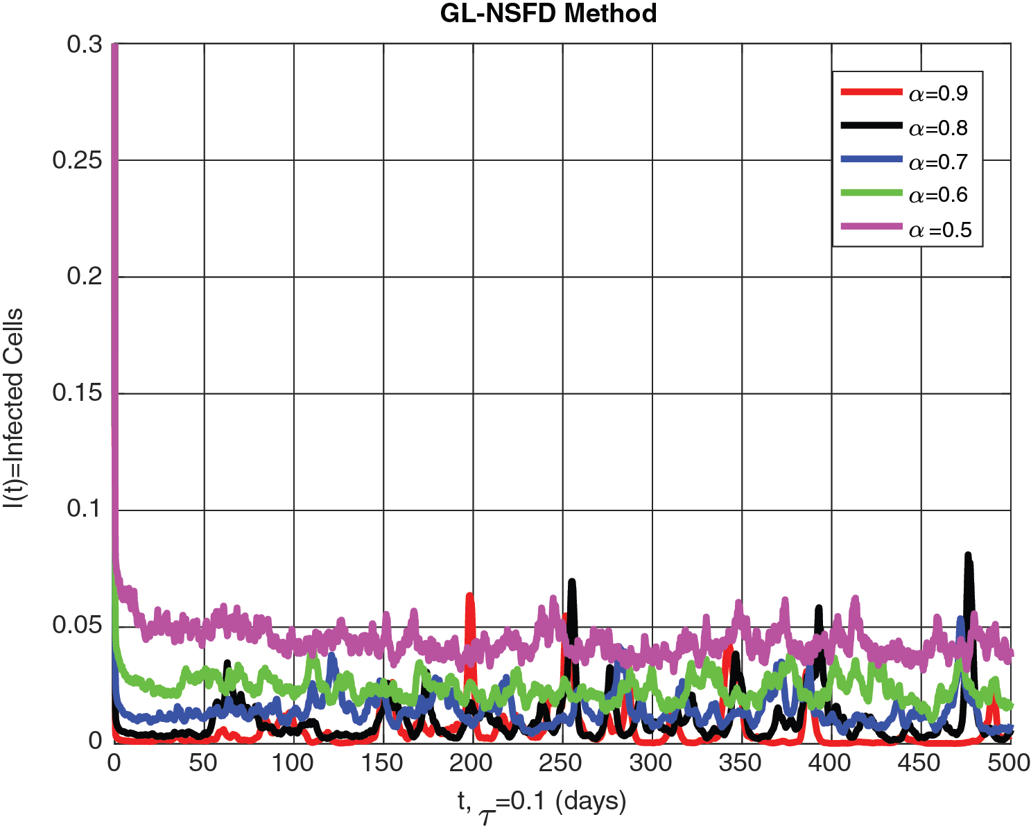
Figure 4: The infected cells are shown graphically for different values of fractional order

Figure 5: The immune cells’ graphical behavior for different values of fractional order
In this article, we have developed a stochastic fractional delayed model to examine the dynamics of leukemia. Thus, it provides significant insights into both the progression of the disease and its control mechanisms. The model (which is quite complex) is specifically designed to capture the intricate dynamics related to leukemia progression. It integrates delays and stochastic processes to address the variability that is inherent in the disease’s advancement. A crucial aspect of this research involves identifying and analyzing both free and present equilibrium points, respectively. The computation of the reproduction number is essential for understanding the threshold behavior that determines whether the disease will persist or decline within a population. The stability of these equilibrium points (both locally and globally) is examined rigorously. Local stability, however, ensures the immediate response of the system around an equilibrium point. Global stability guarantees the system’s long-term behavior. Interestingly, the results reveal critical conditions under which leukemia can be controlled or even eradicated. Although some parameters influence this stability, the underlying mechanisms remain complex. This complexity is vital because it shapes our understanding of potential therapeutic approaches. Sensitivity analysis further enhances these findings by identifying the key parameters that have the most significant influence on disease dynamics. This is crucial for developing targeted interventions (to effectively control the spread of leukemia). The GL-NSFD method is utilized for numerical simulations; it ensures the model’s positivity and boundedness are both essential for maintaining biological relevance. The GL-NSFD method guarantees that solutions stay within realistic bounds, thus avoiding unphysical behavior in the simulation. However, graphical simulations are employed to substantiate the numerical findings, providing a visual representation of the model’s behavior under various conditions. These simulations not only confirm the theoretical results but also demonstrate the practical applicability of the model for understanding leukemia dynamics. Although this research contributes valuable insights into leukemia modeling, it offers potential avenues for more effective treatment (and disease management strategies) because it lays the groundwork for future investigations.
Acknowledgement: This research was partially supported by the Fundacao para a Ciencia e Tecnologia, FCT, under the project https://doi.org/10.54499/UIDB/04674/2020 (accessed on 1 January 2025). Also, the authors were also partial supported by the Center for Research and Development in Mathematics and Applications (CIDMA) through the Portuguese Foundation for Science and Technology, references UIDB/04106/2020 and UIDP/04106/2020.
Funding Statement: This research was partially supported by the Fundação para a Ciência e Tecnologia, FCT, under the project https://doi.org/10.54499/UIDB/04674/2020 (accessed on 1 January 2025).
Author Contributions: Ali Raza: Conceptualization, Investigation, Data curation, Writing—original draft. Feliz Minhós: Project administration, Conceptualization, Investigation, Funding acquisition, Resources, Supervision. Umar Shafique and Muhammad Mohsin: Software, Writing—original draft & review & editing. All authors reviewed the results and approved the final version of the manuscript.
Availability of Data and Materials: All the data used and analyzed is available in the manuscript.
Ethics Approval: Not applicable.
Conflicts of Interest: The authors declare no conflicts of interest to report regarding the present study.
References
1. Khatun MS, Biswas MHA. Mathematical analysis and optimal control applied to the treatment of leukemia. J Appl Math Comput. 2020;64(1):331–53. doi:10.1007/s12190-020-01357-0. [Google Scholar] [CrossRef]
2. Cadot S, Audebert C, Dion C, Ken S, Dupré L, Largeaud L, et al. New pharmacodynamic parameters linked with ibrutinib responses in chronic lymphocytic leukemia: prospective study in real-world patients and mathematical modeling. PLoS Med. 2024;21(7):e1004430. doi:10.1371/journal.pmed.1004430. [Google Scholar] [PubMed] [CrossRef]
3. Kumar R, Shah SR, Stiehl T. Understanding the impact of feedback regulations on blood cell production and leukemia dynamics using model analysis and simulation of clinically relevant scenarios. Appl Math Model. 2024;129:340–89. doi:10.1016/j.apm.2024.01.048. [Google Scholar] [CrossRef]
4. Parajdi LG, Bai X, Kegyes D, Tomuleasa C. A mathematical model of clonal hematopoiesis explaining phase transitions in myeloid leukemia. arXiv:2401.05316. 2024. [Google Scholar]
5. Brunetti M, Iasenza IA, Jenner AL, Raynal NJM, Eppert K, Craig M. Mathematical modeling of clonal reduction therapeutic strategies in acute myeloid leukemia. Leuk Res. 2024;140(4):107485. doi:10.1016/j.leukres.2024.107485. [Google Scholar] [PubMed] [CrossRef]
6. Nicolini DL, Lepoutre T. Stability analysis of a model of INTERACTION between the immune system and cancer cells in chronic myelogenous leukemia. Bull Math Biol. 2018;80(5):1084–110. doi:10.1007/s11538-017-0272-7. [Google Scholar] [PubMed] [CrossRef]
7. Serrano S, Barrio R, Martínez-Rubio Á, Belmonte-Beitia J, Pérez-García VM. Understanding the role of B-cells in CAR T-cell therapy in leukemia through a mathematical mode. arXiv:2403.00340. 2024. [Google Scholar]
8. Dariva K, Lepoutre T. Influence of the age structure on the stability in a tumor-immune model for chronic myeloid leukemia. Math Model Nat Phenom. 2024;19:1. doi:10.1051/mmnp/2023034. [Google Scholar] [CrossRef]
9. Shah K, Ahmad S, Ullah A, Abdeljawad T. Study of chronic myeloid leukemia with T-cell under fractal-fractional order model. Open Phys. 2024;22(1):20240032. doi:10.1515/phys-2024-0032. [Google Scholar] [CrossRef]
10. Lai X, Jiao X, Zhang H, Lei J. Computational modeling reveals key factors driving treatment-free remission in chronic myeloid leukemia patients. npj Syst Biol Appl. 2024;10(1):45. doi:10.1038/s41540-024-00370-4. [Google Scholar] [PubMed] [CrossRef]
11. Zaagan AA, Mahnashi AM. Analysis of leukemia and forest fires data using new Poisson Quasi-Shanker distribution. Alex Eng J. 2024;104(3):701–9. doi:10.1016/j.aej.2024.08.012. [Google Scholar]
12. Bose P, Bandyopadhyay S. A comprehensive assessment and classification of acute lymphocytic leukemia. Math Comput Appl. 2024;29(3):45. doi:10.3390/mca29030045. [Google Scholar] [CrossRef]
13. Li J, Pavlov S, Stakhov O. Expert systems for analysis of biomedical information in the diagnosis of acute leukemia. Інформаційні Технології Та Комп’ютерна Інженерія. 2024;59(1):157–64. [Google Scholar]
14. Miotto M, Scalise S, Leonetti M, Ruocco G, Peruzzi G, Gosti G. A size-dependent division strategy accounts for leukemia cell size heterogeneity. Commun Phys. 2024;7(1):248. doi:10.1038/s42005-024-01743-1. [Google Scholar] [CrossRef]
15. Niño-López A, Chulián S, Martínez-Rubio Á, Blázquez-Goñi C, Rosa M. Mathematical modeling of leukemia chemotherapy in bone marrow. Math Model Nat Phenom. 2023;18:21. doi:10.1051/mmnp/2023022. [Google Scholar] [CrossRef]
16. Abdullah R, Badralexi I, Halanay A. Stability analysis in a new model for desensitization of allergic reactions induced by chemotherapy of chronic lymphocytic leukemia. Mathematics. 2023;11(14):3225. doi:10.3390/math11143225. [Google Scholar] [CrossRef]
17. Khan H, Alzabut J, Alfwzan WF, Gulzar H. Nonlinear dynamics of a piecewise modified ABC fractional-order leukemia model with symmetric numerical simulations. Symmetry. 2023;15(7):1338. doi:10.3390/sym15071338. [Google Scholar] [CrossRef]
18. Pozzati G, Zhou J, Hazan H, Klement GL, Siegelmann HT, Tuszynski JA, et al. A systems biology analysis of chronic lymphocytic leukemia. Onco. 2024;4(3):163–91. doi:10.3390/onco4030013. [Google Scholar] [CrossRef]
19. Jiwani N, Gupta K, Pau G, Alibakhshikenari M. Pattern recognition of acute lymphoblastic leukemia (ALL) using computational deep learning. IEEE Access. 2023;11:29541–53. doi:10.1109/access.2023.3260065. [Google Scholar] [CrossRef]
20. Xiang H, Zhou M, Liu X. An optimal treatment strategy for a leukemia immune model governed by reaction-diffusion equations. J Dyn Control Syst. 2023;29(4):1219–39. doi:10.1007/s10883-022-09621-1. [Google Scholar] [CrossRef]
21. Stiehl T. The multiplicity of time scales in blood cell formation and leukemia: contributions of computational disease modeling to mechanistic understanding and personalized medicine. In: Booß-Bavnbek B, Hesselbjerg Christensen J, Richardson K, Vallès Codina O, editors. Multiplicity of time scales in complex systems: challenges for sciences and communication I. Cham, Switzerland: Springer International Publishing; 2023. p. 327–99. doi: 10.1007/16618_2023_73. [Google Scholar] [CrossRef]
22. Alsakaji HJ, Rihan FA, Udhayakumar K, El Ktaibi F. Stochastic tumor-immune interaction model with external treatments and time delays: an optimal control problem. Math Biosci Eng. 2023;20(11):19270–99. doi:10.3934/mbe.2023852. [Google Scholar] [PubMed] [CrossRef]
23. Rihan FA, Udhayakumar K. Fractional order delay differential model of a tumor-immune system with vaccine efficacy: stability, bifurcation and control. Chaos Solitons Fractals. 2023;173(4):113670. doi:10.1016/j.chaos.2023.113670. [Google Scholar] [CrossRef]
24. Moore H, Li NK. A mathematical model for chronic myelogenous leukemia (CML) and T cell interaction. J Theor Biol. 2004;227(4):513–23. doi:10.1016/j.jtbi.2003.11.024. [Google Scholar] [PubMed] [CrossRef]
Cite This Article
 Copyright © 2025 The Author(s). Published by Tech Science Press.
This work is licensed under a Creative Commons Attribution 4.0 International License , which permits unrestricted use, distribution, and reproduction in any medium, provided the original work is properly cited.
 Downloads
 Citation Tools