Modeling of CO₂ Emission for Light-Duty Vehicles: Insights from Machine Learning in a Logistics and Transportation Framework

1  Introduction

1.1 Problem Statement

With the rapid growth of economic and social activities worldwide, Light-Duty Vehicles (LDVs), including vans, pickup trucks, and small delivery vehicles, have become essential for passenger mobility and the sustainable transport of goods [1]. LDVs, typically defined as vehicles with a gross weight rating of 10,000 pounds or less, play a crucial role in logistics and transportation systems. Their importance has grown significantly in response to the rise of e-commerce, particularly in last-mile delivery operations, where timely and high-quality delivery is paramount. However, LDVs are also among the major contributors to air pollution and environmental degradation [2]. Due to their reliance on internal combustion engines (mainly powered by diesel and gasoline), LDVs emit substantial amounts of air pollutants such as particulate matter (PM2.5 and PM10), carbon monoxide (CO), nitrogen oxide (NOx), unburned hydrocarbons (UHC), and greenhouse gases (CO2 and N2O) [3]. In urban areas, where LDVs are heavily utilized, elevated CO2 emissions, a dangerous Greenhouse Gas (GHG) and a key driver of climate change, demand urgent attention from policymakers and environmental stakeholders [4].

1.2 LDVs’ CO2 Emission Modeling

Modeling and assessing CO2 emissions from transportation, as an essential step in the decision-making process, presents significant complexity due to the multitude of influencing factors [5,6]. Predictive models for vehicle-related CO2 emissions can generally be categorized into statistical models and Artificial Intelligence (AI) models. Traditional statistical models, such as Autoregressive-Integrated Moving Average (ARIMA), Seasonal ARIMA with exogenous factors (SARIMAX), and the Holt-Winters model, are typically applied to annual datasets, as they primarily capture long-term trends. In addition, these models require the dataset to be stationary, limiting their flexibility and application [7]. To overcome the limitations of traditional prediction methods, AI techniques have emerged as an efficient tool offering the ability to model processes involving vast amounts of data and detect hidden patterns.

Researchers and practitioners have approached the modeling and prediction of CO2 emissions released by LDVs from two main perspectives, depending on the datasets used and the prediction/modeling tools adopted. Some studies have focused on vehicle assessment using data collected from Portable Emission Measurement System (PEMS) devices embedded in those vehicles [8]. In contrast, other studies have utilized large-scale compiled at national or international levels, encompassing a wide variety of vehicle types and usage patterns [9]. This latter approach offers the advantage of broader applicability, as similar vehicle models tend to exhibit consistent CO2 emission patterns across different countries, providing a more generalized understanding of emission behaviors.

In this context, the main aim of the current study is to help fill the applied research gap by analyzing and comparing CO2 emissions from various LDVs, thereby enhancing understanding of their impact on climate change and environmental issues. By utilizing a large-scale dataset that covers LDVs from different manufacturers and applying multiple ML algorithms under consistent conditions, the study evaluates the predictive accuracy of various models for CO2 emissions and identifies the most influencing variables. In practice, such a comparative modeling approach is expected to valuable insights into CO2 emissions across LDV types and support informed decision-making to reduce emissions in the global vehicle market [10].

1.3 Paper Outline

The remainder of this article is organized as follows. Section 2 includes an extensive literature review as well as the contributions of the paper. Section 3 explores the dataset used in addition to its exploratory analysis. Section 4 is allocated to the proposed methodology. In Section 5, the results and their discussion are provided. Finally, Section 6 includes the conclusions of the study and its perspectives.

2  Literature Review

CO2 emissions from vehicles are classified as among the most significant GHGs and impactful contributors to climate change. Following the Paris agreement, GHG emissions are expected to be reduced by 40%, below 1990 levels by 2030 [11]. Researchers around the world were extensively interested in developing practical models to predict CO2 emissions as correlated with many attributes, including the fuel type utilized, the engine size, the number of cylinders, etc. In addition, many CO2 emission related studies were based on individual vehicles and therefore concentrated on immediate attributes, including driver behavior, road conditions, and climatic factors. However, most studies focused on certain types of vehicles seen in their broader scope. In what follows, the focus will be on the studies that use AI techniques, including the main classes of methods, namely, Machine Learning (ML) and Deep Learning (DL). The focus will therefore be on the study objective, the dataset utilized, the models/methods employed, the achieved performance metrics, as well as their limitations. The main objective of this approach is to be well-situated with the contributions of the current study against existing ones on the same topic. Earlier research efforts on this topic are thoroughly summarized hereafter in Table 1.

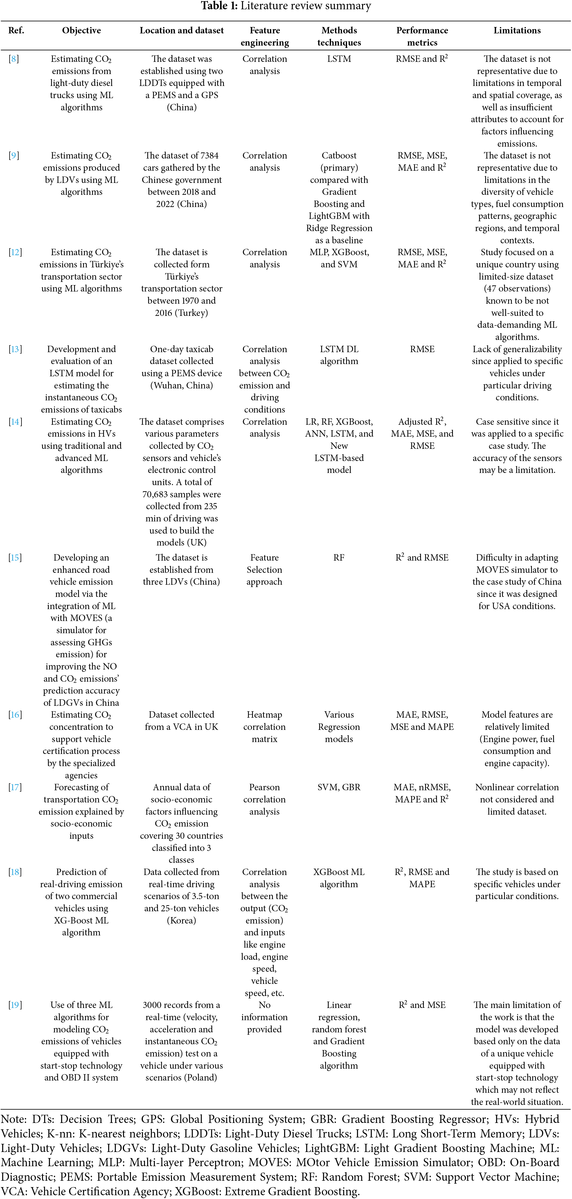
Based on the summarized studies of Table 1, it can be noticed that the problem of CO2 emission concerns researchers worldwide due to its negative effect on the climate and environment. The conducted studies have comprehensively concentrated on macroscopic and microscopic levels, respectively, considering thorough datasets collected at national or international levels or vehicle-specific datasets collected through PEMS devices. Among the second class of works, the study in [20] assessed NOx/CO2 emission under particular driving scenarios. The results were reported to be promising in improving air quality in Wuhan (China). In the same direction, the study carried out in [21] investigated the ability to estimate the CO2 emissions for two vehicles based on PEMS data and Long Short-Term Memory (LSTM). Although they are relevant to the current topic, the two research works have the limitation of being applied to specific case studies and therefore, they lack generalization ability with case-sensitive findings. Moreover, a few studies have considered annual datasets analyzing the effect of socio-economic factors impacting transportation’s CO2 emission. A common practice was to consider feature engineering based on the well-known Pearson (linear) correlation. Meanwhile, none of the studies have considered nonlinear correlation indices such as Spearman and Kendall. The developed prediction/modeling techniques were found to range from simple regression to sophisticated ML algorithms. The performance indicators obtained were found to be case-sensitive depending on the size of the dataset, the techniques/methods employed, and the computational resources. In terms of limitations, the common one was the special cases of particular vehicles’ difficulty generalizable to other ones under different conditions. In addition, in most cases, the size of the dataset was limited which may not provide high accuracy when ML/DL algorithms were employed as they are known to be data-hungry. In line with the above literature review, the present paper focuses on the prediction/modeling of LDVs-related CO2 emissions based on six, complementary, ML algorithms and a comprehensive dataset including several LDVs from various brands and sizes. Therefore, this work aims to fill specific research and methodological gaps in the literature. Specifically:

1)   Various models for CO2 emissions worldwide have been investigated in the literature, ranging from simple linear to highly non-linear approaches. This work aims to explore the capabilities of six models, including some additional ones that have not been previously examined.

2)   Numerous feature engineering techniques combined with data-driven models have been proposed and validated in the literature for predicting CO2 emissions worldwide, offering comprehensive frameworks for tackling this prediction task. This work seeks to contribute to the body of knowledge by introducing an additional predictive modeling framework that accurately addresses CO2 prediction. It explores various ML models, ranging from linear to non-linear, that complement those previously studied in the literature, ensuring proper hyperparameter optimization. Additionally, it incorporates linear and non-linear correlation (Spearman and Kendall), evaluates performance metrics, and statistically analyzes the influence of different vehicle attributes on CO2 emissions.

3  Data Description

The dataset, sourced by1, has been investigated in this work to address the work’s objectives. The dataset was obtained from Kaggle and cross-referenced with the Canadian Government’s open data portal. The dataset comprises 7385 vehicles, each with various attributes/features relevant to its specification (e.g., vehicle manufacturer), performance (e.g., number of cylinders), fuel efficiency (e.g., fuel consumption), and environmental impact (e.g., CO2 emission).

The dataset used in this study represents a wide range of manufacturers and LDV brands commonly used worldwide. Our analysis is based on the assumption that, in general, new LDVs exhibit consistent CO2 emission behavior regardless of the location/country in which they are operated. As a common practice, after a certain period of use, and subsequently at regular intervals, (depending on the country (regional level) local standards), LDVs undergo inspection, and any violations must be addressed by the vehicle owner according to the local regulations. Therefore, the dataset is used to model the CO2 emission levels based on the selected features, assuming that new vehicles have similar emission patterns regardless of location. Local or regional regulations should be applied systematically and regularly after the LDV is being used. Notably, the dataset used in this study contains no missing data.

Note here that the dataset does not include the vehicle usage conditions, such as mileage, road conditions and climate. Although those conditions are known to have a high impact on CO2 emission and this effect may be explored by collecting real datasets of specific vehicles as carried out in many papers among those we cited in this paper (examples can be found in [12–14]). However, in the current study, this is considered a limitation since it covers only specific vehicles under specific conditions which therefore lacks generalization ability. Meanwhile, our paper covers several brands from many manufacturers while focusing on the technical specifications of the investigated vehicles as well as their effect on CO2 emission patterns. This may allow far away better generalization. In conclusion, the vehicle usage conditions, and the vehicle technical specifications are conceptually different although tackling the same problem of CO2 emission.

For clarity, the attributes/features are detailed in Table 2. The fuel consumption in combined conditions represents a standardized approximation of an average driver’s typical usage pattern, with a ratio of 55% City and 45% Highway driving.

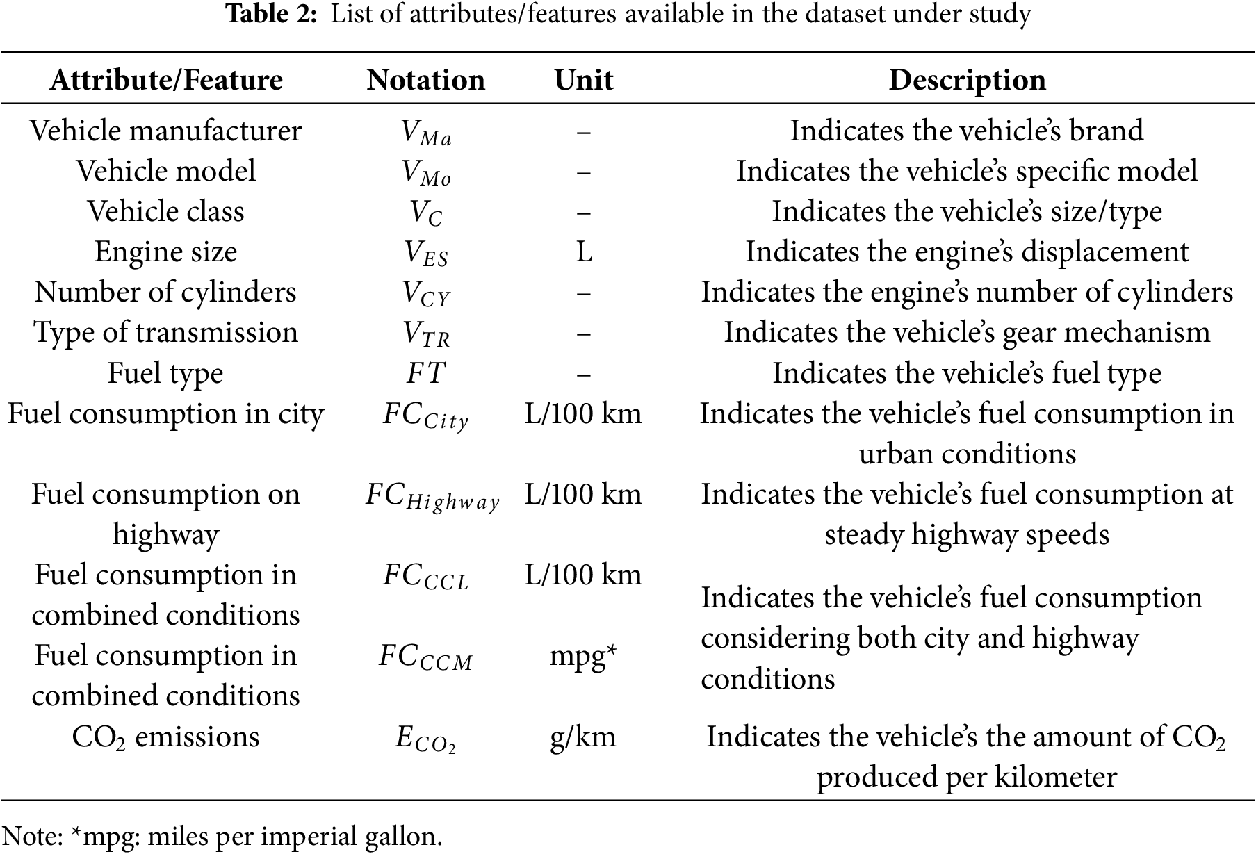
Among the 12 available attributes/features, there are 5 categorical variables and 7 numerical variables. Specifically, the vehicle manufacturer (comprising 42 unique brands), model (comprising 2047 specific models), class (comprising 16 sizes/types), type of transmission including the number of gears (comprising 27 transmission types), and fuel type (comprising 5 specific fuel types) are categorical variables whereas the remaining 7 are numerical variables, whose values vary based on the nature of each attribute/feature.

For instance, among the available categorical variables, examples include ACURA, AUDI, BMW, VOLVO, and TOYOTA (for the vehicle’s manufacturer); ILX, A4, 320i, CAMRY, and S60 (for vehicle’s model); COMPACT, MID-SIZE, SUV-SMALL, and FULL-SIZE (for vehicle’s class); Automatic with Select Shift (AS), Manual (M), and Continuously Variable (AV), including number of gears (from 3 to 10) (for vehicle’s transmission type); and Regular Gasoline (X), Premium Gasoline (Z), and Diesel (D) (for vehicle’s fuel type). It is worth mentioning that the categorical attributes were encoded into numeric values using label encoding to ensure compatibility with the ML models used in the subsequent prediction analysis. For clarity, Figs. 1–5 illustrate the distribution of these five categorical variables in order. Although there are 2047 unique vehicle models, only the top 50 most frequent ones are shown in Fig. 2 for better readability.

Figure 1: The number of events distributed by vehicle’s manufacturer

Figure 2: The number of events distributed by vehicle model. The highest 50 events are shown for clarity

Figure 3: The number of events distributed by vehicle’s class

Figure 4: The number of events distributed by vehicle’s transmission type

Figure 5: The number of events distributed by vehicle’s fuel type

Similarly, among the available numerical variables, the ranges of values include [0.9–8.4] (for engine size), [3–16] (for number of cylinders), [4.2–30.6] (for fuel consumption in city), [4–20.6] (for fuel consumption on highway), [4.1–26.1] (for fuel consumption in combined conditions, measured in L/100 km), [11–69] (for fuel consumption in combined conditions, measured in mpg), and [96–522] (for CO2 emissions). For clarity, Figs. 6–11 illustrate the histograms of these seven numerical variables in order.

Figure 6: The histogram of the “engine size”

Figure 7: The histogram of the “number of cylinders”

Figure 8: The histogram of the “fuel consumption in city”

Figure 9: The histogram of the “fuel consumption on highway”

Figure 10: The histogram of the “fuel consumption in combined conditions, measured in L/100 km”

Figure 11: The histogram of the “fuel consumption in combined conditions, measured in mpg”

To effectively present the statistical distribution of the available attributes/features, Fig. 12 illustrates the boxplot of all normalized features in order, including CO2 emissions. From Fig. 12, it is evident that CO2 emissions and the corresponding fuel consumption features exhibit significant variability and numerous outliers compared to other features, such as engine size. This indicates potential correlations between CO2 emissions and other features, which will be explored later in subsequent sections of this work. To effectively address the correlations between variables, outliers were eliminated using the Interquartile Range (IQR) method. Outliers are typically defined as data points that fall below the 1st Quartile (Q1) or above the 3rd Quartile (Q3) by more than 1.5 times the IQR. As a result, 960 data points were excluded from the subsequent analysis, leaving a total of 6425 data points.

Figure 12: Boxplots of the whole variables in the dataset

4  The Proposed Methodology

This section presents the methodology proposed in this work to develop a predictive model for the CO2 emissions (g/km) based on the historical recorded vehicle design, models, performance, fuel consumption, and their associated CO2 emissions of the case under study. The refined version of the dataset, after excluding the 960 outlier data points and transforming the categorical attributes into numeric format, is referred to as Xred1, with a size of 6425×12.

Specifically, the proposed methodology is structured in three systematic and chronological steps, as depicted in Fig. 13. Specifically, it begins with statistical and correlation analysis to better understand the association levels and impact of each attribute on CO2 emissions, while also refining the dataset by eliminating potentially redundant or irrelevant features (Step 1). Once these association levels are identified and the dataset is refined, the methodology progresses to establish dataset variants, aiming to comprehensively determine the set of attributes that maximize the predictability of CO2 emissions (Step 2). To achieve this, the six investigated ML models are developed and properly optimized using each dataset variant while computing various performance metrics from the literature (Step 3). In detail:

Figure 13: The proposed predictive modelling approach of CO2 emissions

Step 1. Statistical and Correlation Analysis. This step entails statistically analyzing the historically available dataset to better understand the association level and impact of each attribute on CO2 emissions. To this aim, the distributions of the emissions per unique values of the input attributes are to be identified and the correlation (r) between them is to be computed. For this latter, three correlation metrics are employed to compute the association levels with the emissions, aiming to effectively identify the set of attributes that largely affect the CO2 emissions while developing the predictive models. Specifically, Pearson [22], Spearman [23], and Kendall [24] correlation coefficients are investigated to compute the relationships and gain a comprehensive overview of the interdependencies among the combined categorical and numerical attributes/features. Practically the Pearson correlation is effectively used for numerical attributes in which the relationship is crucial, whereas Spearman and Kendall are more suitable for ordinal data or non-linear relationships, as they assess the strength and direction of monotonic associations. Last, based on the computed correlation metrics, correlation heatmaps are established to visually interpret the attribute/feature relationships and to initially identify attributes/features exhibiting high multicollinearity, for establishing dataset variants (Step 2) aimed at effective CO2 emissions prediction (Step 3).

Step 2. Feature Refinement and Dataset Variants Establishment. Once the correlation metrics are computed in Step 1, the established correlation heatmaps are initially used to visually identify and remove highly correlated independent attributes/features from the overall dataset. Subsequently, a Variance Inflation Factor (VIF) analysis is performed on the reduced dataset to confirm that multicollinearity has been effectively eliminated and that the remaining attributes/features offer independent predictive power. Once the refined feature set is finalized, one can establish dataset variants to effectively identify the set of attributes/features that might have an impact on the predictability of CO2 emissions for any type of vehicle. Specifically, the retained attributes after correlation- and VIF-based filtering are to be used to establish a reduced-version dataset (Xred1). From this reduced-version dataset, additional reduced-version dataset variants are established by progressively excluding features one by one, i.e., Xred2, Xred3, and so on, upon reaching a dataset that contains the attribute of the largest impact on CO2 emissions. The objective is to establish dataset variants that strike a balance between feature complexity and the predictive performance of CO2 emissions in the next step (i.e., Step 3). It is worth mentioning that the categorical attributes were converted to numeric indices within each dataset variant to ensure their effective utilization in the ML models’ development of of Step 3.

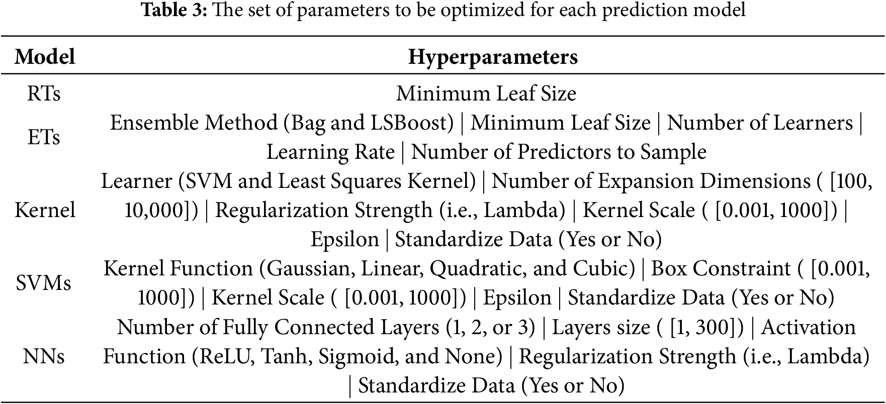
Step 3. Predictive Model Development and Validation. For each established dataset, a set of data-driven models are investigated to accurately estimate the CO2 emissions based on a set of selected attributes identified in each dataset variant. The models range from simple Linear Regression (LR) models to more advanced non-linear models, including Regression Trees (RTs), Ensemble of Trees (ETs), Kernel Approximation Models (Kernel), Support Vector Machines (SVMs), and Neural Networks (NNs). The models are built while investigating various potential configurations to ensure they have the optimal configuration (i.e., hyperparameters) of each model. That is, the models are optimized in terms of their internal configurations (i.e., hyperparameters), resorting to Bayesian Optimization (BO) optimizer. Specifically, Table 3 summarizes the set of parameters to be optimized while developing the prediction models. The LR models include identifying the best LR scheme among Linear, Interactions, Robust, and Stepwise LR variants. Last, the Regression Learner Application available in MATLAB® is being used to devise the models2 .

Each dataset variant is divided following 80–20 rule for the train and test portions. The 80% portion will be subjected to a 5-fold cross validation approach to ensure robustness while developing the prediction models. The 80–20 portions will be the same among the whole dataset variants for a fair comparison with the sole difference in the number of attributes to be used as inputs to the prediction models. Furthermore, the impact of attribute standardization (zero-mean normalization) has also been investigated across the evaluated models.

Further, the models are compared against each other through a set of standard performance metrics, including the Root Mean Square Error (RMSE) (in g/km) (Eq. (1)), Mean Absolute Error (MAE) (in g/km) (Eq. (2)), Mean Absolute Percentage Error (MAPE) (in %) (Eq. (3)), Coefficient of Determination (R2) (in %) (Eq. (4)), and Computational Time (in seconds).

RMSE=1n∑i=1n(ECO2i−E^iCO2)2(1)

MAE=1n∑i=1n|ECO2i−E^iCO2|(2)

MAPE=100n∑i=1n|ECO2i−E^iCO2ECO2i|(3)

R2=1−∑i=1n(ECO2i−E^iCO2)2∑i=1n(ECO2i−E¯CO2)2(4)

where i is a general index of a validation data point (i=1,…,n), n is the total number of validation data points, ECO2i and E^iCO2 are the actual and estimated i-th CO2 emission values, respectively, and E¯CO2 is the average value of the actual CO2 emissions across the validation dataset.

The model’s configuration that achieves the best predictability of the CO2 emissions on the 80% validation portion will be later used to evaluate its goodness and effectiveness on the fixed unseen 20% test portion. Subsequently, insights can be drawn on each model’s predictability.

5  Results and Discussion

In this section, the application results of the proposed approach to the case study at hand are presented step-by-step.

The refined dataset that comprises the whole available attributes/features (Xref) of 6425 data points is statistically analyzed and the correlation values between the 11 independent attributes to the CO2 emissions are computed using the three-correlation metrics being investigated in this work (i.e., Step 1).

The Pearson correlation measures the linear association between individual numeric attributes and CO2 emissions, while the Spearman and Kendall correlations capture monotonic relationships between the entire set of numeric and encoded categorical attributes and CO2 emissions. For clarity and conciseness, only the Kendall correlation heatmap is presented in Fig. 14, as the correlation results were found to be largely consistent across all three correlation methods. For reference, the Pearson and Spearman correlation heatmaps are provided in Appendix A. From Fig. 14, one can cite the following insights:

Figure 14: Kendall correlation heatmap

-   The Vehicle Manufacturer (VMa), Vehicle Model (VMo), Vehicle Class (VC), and the Number of Transmission (VTR) show very weak correlations with each other and with most other attributes, suggesting that they are largely independent and do not contribute significantly to multicollinearity.

-   The Vehicle Engine Size (VES) and Number of Cylinders (VCY) show moderate correlations with each other, indicating partial redundancy, i.e., mechanical related attributes, with significant contribution to multicollinearity.

-   The Fuel Consumption (in City (FCCity), on Highway (FCHighway), and in Combined Conditions (FCCCL and FCCM)) show the highest correlations among each other (i.e., > 0.78), indicating high redundancy, with a significant contribution to multicollinearity.

-   The fuel consumption attributes (FCCCL,FCCCM,FCCity, and FCHighway), followed by Vehicle Engine Size (VES), Number of Cylinders (VCY), Number of Transmission (VTR), Vehicle Class (VC), Fuel Type (FT), Vehicle Manufacturer (VMa), and Vehicle Model (VMo), show varying degrees of correlation with CO2 emissions, with corresponding Kendall correlation coefficients of 0.9776, −0.9703, 0.9223, 0.8617, 0.6823, 0.6985, −0.2252, 0.2078, 0.1658, −0.09719, and 0.08034, respectively. In practice:

-   Higher fuel consumption is directly associated with higher CO2 emissions.

Larger engines with large numbers of cylinders consume more fuel, thereby emitting more CO2.

-   The Vehicle Class (VC) indirectly affects CO2 emissions by influencing engine size and fuel consumption.

-   The Number of Transmission (VTR) impacts fuel consumption efficiency. For instance, specific transmission types (e.g., manual) improve fuel efficiency compared to other types (e.g., automatic), thereby contributing to lower CO2 emissions.

-   Fuel Type (FT) reflects differences in combustion properties, which influence fuel efficiency and emissions.

-   Vehicle Manufacturer (VMa) and Vehicle Model (VMo) indicate different vehicle designs, performance, and technological variations, thereby impacting, indirectly the CO2 emissions.

To gain deeper insights into the impact of each attribute and its unique values on CO2 emissions (ECO2), Figs. 15–25 illustrate the attributes’ effects, starting with the categorical variables (Figs. 15–19) and followed by the numerical variables (Figs. 20–25). These figures highlight the average CO2 emissions (depicted as bars) and their associated standard deviation values (depicted as error bars). From the figures, the following insights can be drawn:

Figure 15: The distribution of CO2 emissions (ECO2) across the available unique vehicle manufacturers (VMa)

Figure 16: The distribution of CO2 emissions (ECO2) across the available unique vehicle models (VMo). The highest 50 emissions are shown for clarity

Figure 17: The distribution of CO2 emissions (ECO2) across the available unique vehicle classes (VC)

Figure 18: The distribution of CO2 emissions (ECO2) across the available unique vehicle transmission types (VTR)

Figure 19: The distribution of CO2 emissions (ECO2) across the available unique fuel types (FT)

Figure 20: The distribution of CO2 emissions (ECO2) across the available unique numbers of cylinders (VCY)

Figure 21: The distribution of CO2 emissions (ECO2) across the available unique engine sizes (ES)

Figure 22: The distribution of CO2 emissions (ECO2) across the available unique fuel consumption in City (FCCity)

Figure 23: The distribution of CO2 emissions (ECO2) across the available unique fuel consumption on highway (FCHighway)

Figure 24: The distribution of CO2 emissions (ECO2) across the available unique fuel consumption in combined conditions (L/100 km) (FCCCL)

Figure 25: The distribution of CO2 emissions (ECO2) across the available unique fuel consumption in combined conditions (mpg) (FCCCM)

-   It is apparent that BUGATTI vehicles contribute the most to CO2 emissions, with around 500 g/km, compared to SMART vehicles, which emit approximately 180 g/km. Both brands exhibit minimal variability in their CO2 emissions. This disparity can be attributed to differences in vehicle design, performance, and other contributing factors such as engine size, fuel type, and technical specifications. (Fig. 15). Similarly, individual vehicle models show varying levels of CO2 emissions, with the CHIRON model exceeding 500 g/km, compared with the other models whose emissions are less than 500 g/km. Again, this can be attributed to variations in vehicle design, performance, and additional contributing factors such as engine size, fuel type, and other specifications (Fig. 16).

-   In Fig. 17, it is evident that the vehicle class (VC) significantly impacts CO2 emissions. For instance, VAN-PASSENGER class exhibits the highest average emissions, reaching around 400 g/km. In contrast, the STATION WAGON-SMALL class has substantially lower emissions, averaging less than 200 g/km. This variation highlights the importance of vehicle class in determining environmental impact in terms of CO2 emissions.

-   It is apparent that vehicles with A (Automatic), AM (Automated Manual), or AS (Automatic with select Shift) transmissions generally exhibit higher CO2 emissions compared to those with M (Manual) and AV (Continuously Variable) transmissions. However, no specific trend is observed for the number of gears, likely due to the influence of additional attributes (Fig. 18).

-   It is apparent that vehicles using E85 (ethanol) and Z (premium gasoline) fuel tend, on average, to exhibit higher CO2 emissions, followed by X (regular gasoline) and D (diesel) fuel (Fig. 19). This can be justified by the differences in combustion efficiency and energy content across the five different fuel types as well as the number of available events for each fuel type, i.e., 1 event for N (natural gas) fuel, as depicted in Fig. 5.

-   From Fig. 20, as expected, the number of cylinders (VCY) increases, ranging from 3 to 16 cylinders, and the CO2 emissions also increase from around 180 g/km to more than 500 g/km of emissions, respectively.

-   As the engine size (ES) increases, the CO2 emissions (ECO2) also increase, as expected (Fig. 21).

-   As long as fuel consumption (FC) (city (FCCity), highway (FCHighway), or combined conditions in L/100 km (FCCCL)) increases, the CO2 emissions (ECO2) also increase, as expected (Figs. 22–24). Conversely, as the fuel consumption in combined conditions, measured in mpg (FCCCM), increases the associated CO2 emissions (ECO2) decrease, as expected (Fig. 25). The figures illustrate the distribution of CO2 emissions (ECO2) for each fuel consumption value, categorized into intervals.

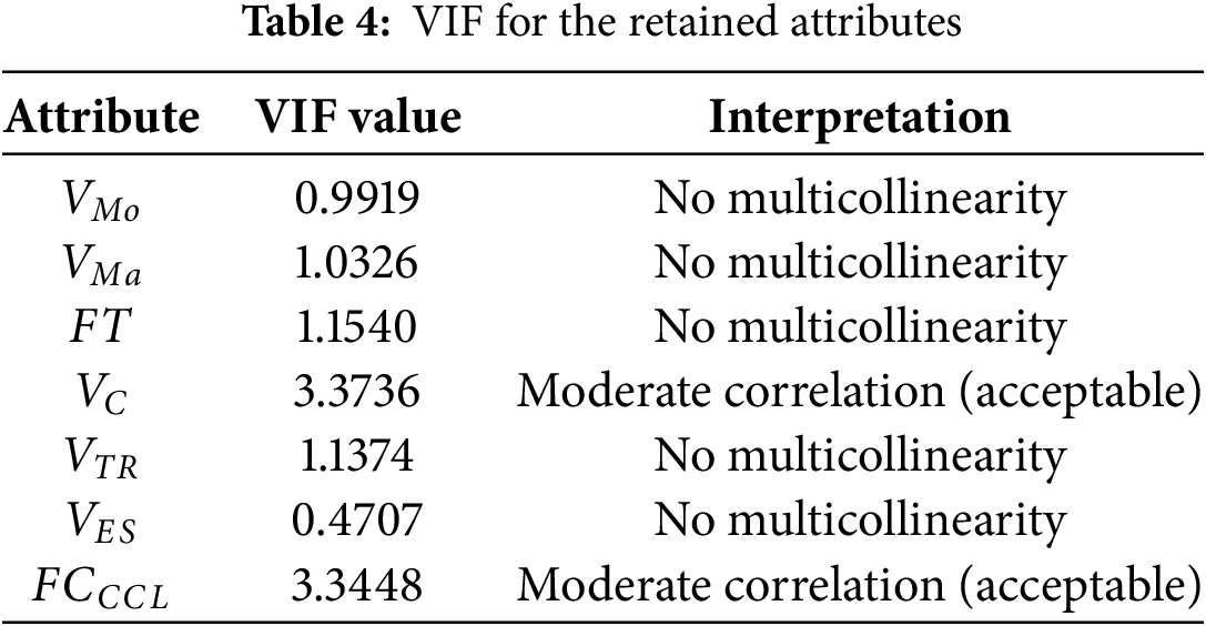
Considering the insights drawn above, the following attributes were retained in the dataset, while the others were excluded due to their significant contributions to multicollinearity. Specifically, FCCCL, VES, VTR, VC, FT, VMa, and VMo were retained, as they were considered non-redundant and independent in relation to CO2 emissions (i.e., Xred1).

To ensure that multicollinearity is avoided, the VIF was computed for the retained attributes. As reported in Table 4, all attributes exhibit VIF values well below the typically accepted threshold of 5. This confirms that multicollinearity is not a concern in the reduced-version dataset (Xred1). Although attributes VC and FCCCL show moderate VIF values (~3.3), they remain within acceptable limits and do not suggest exclusion at this stage.

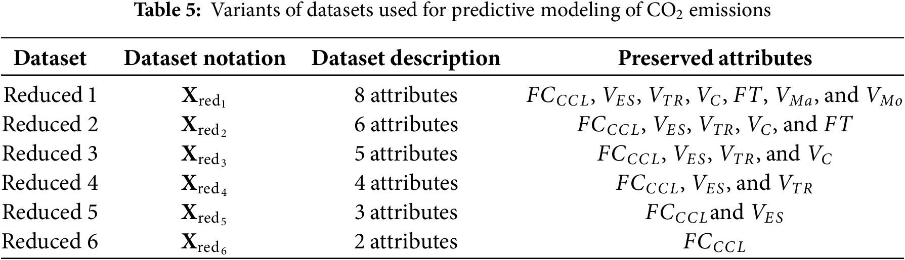
Following this, the reduced-version dataset and its variants are to be used to devise various prediction models aiming to accurately estimate the CO2 emissions (i.e., Step 3). Specifically, the following datasets have been established. The objective is to identify the optimal dataset that comprises the optimal set of attributes that maximizes the prediction accuracy of the CO2 emissions for any type of vehicle, compromising the vehicle specificity and fuel consumption generalizability, that is the complexity of the dataset considered while developing the predictive model:

-   Reduced-Version Dataset 1 (Xred1). It comprises 8 attributes, including the CO2 emissions after excluding the multicollinearity significantly contributing attributes. Specifically, the following attributes are kept as input while developing the predictive model: FCCCL, VES, VTR, VC, FT, VMa, and VMo.

-   Reduced-Version Dataset 2 (Xred2). It comprises 6 attributes, including the CO2 emissions after excluding the least two correlated attributes (VMa and VMo) whose Kendall correlation values are −0.0972 and 0.0830). Specifically, the following attributes are kept as input while developing the predictive model: FCCCL, VES, VTR, VC, and FT.

-   Reduced-Version Dataset 3 (Xred3). It comprises 5 attributes, including the CO2 emissions after excluding the least three correlated attributes (FT, VMa, and VMo) whose Kendall correlation values are 0.1658, −0.0972 and 0.0830). Specifically, the following attributes are kept as input while developing the predictive model: FCCCL, VES, VTR, and VC.

-   Reduced-Version Dataset 4 (Xred4). It comprises 4 attributes, including the CO2 emissions after excluding the least four correlated attributes (VC, FT, VMa, and VMo) whose Kendall correlation values are 0.2078, 0.1658, −0.0972 and 0.0830). Specifically, the following attributes are kept as input while developing the predictive model: FCCCL, VES, and VTR.

-   Reduced-Version Dataset 5 (Xred5). It comprises 3 attributes, including the CO2 emissions after excluding the least five correlated attributes (VTR, VC, FT, VMa, and VMo) whose Kendall correlation values are −0.2252, 0.2078, 0.1658, −0.0972 and 0.0830). Specifically, the following attributes are kept as input while developing the predictive model: FCCCL and VES.

-   Reduced-Version Dataset 6 (Xred6). It comprises 2 attributes, including the CO2 emissions after excluding the least six correlated attributes (VES, VTR, VC, FT, VMa, and VMo) whose Kendall correlation values are 0.6985, −0.2252, 0.2078, 0.1658, −0.0972 and 0.0830). Specifically, the following attributes are kept as input while developing the predictive model: FCCCL.

Table 5 summarizes the set of attributes considered in input to the predictive model across the dataset variants, for clarity.

Once the dataset variants are established, they have been used to develop various prediction models investigated in this work, i.e., LR, RTs, ETs, Kernel, SVMs, and NNs (i.e., Step 3). In this regard, each dataset variant is divided into 80% (5140 data points) and 20% (1285 data points) and the 5-fold cross validation approach is being employed. Tables 6–11 summarize the optimal models’ configurations and the corresponding performance metrics on the validation portion of the 5-fold cross validation approach for Xred1, Xred2, Xred3, Xred4, Xred5, and Xred6, respectively. Indeed, the average computational efforts needed by the simple models, such as the LR and RTs, are much less than those required by the more advanced non-linear models, such as the SVMs and NNs, across the whole dataset variants.

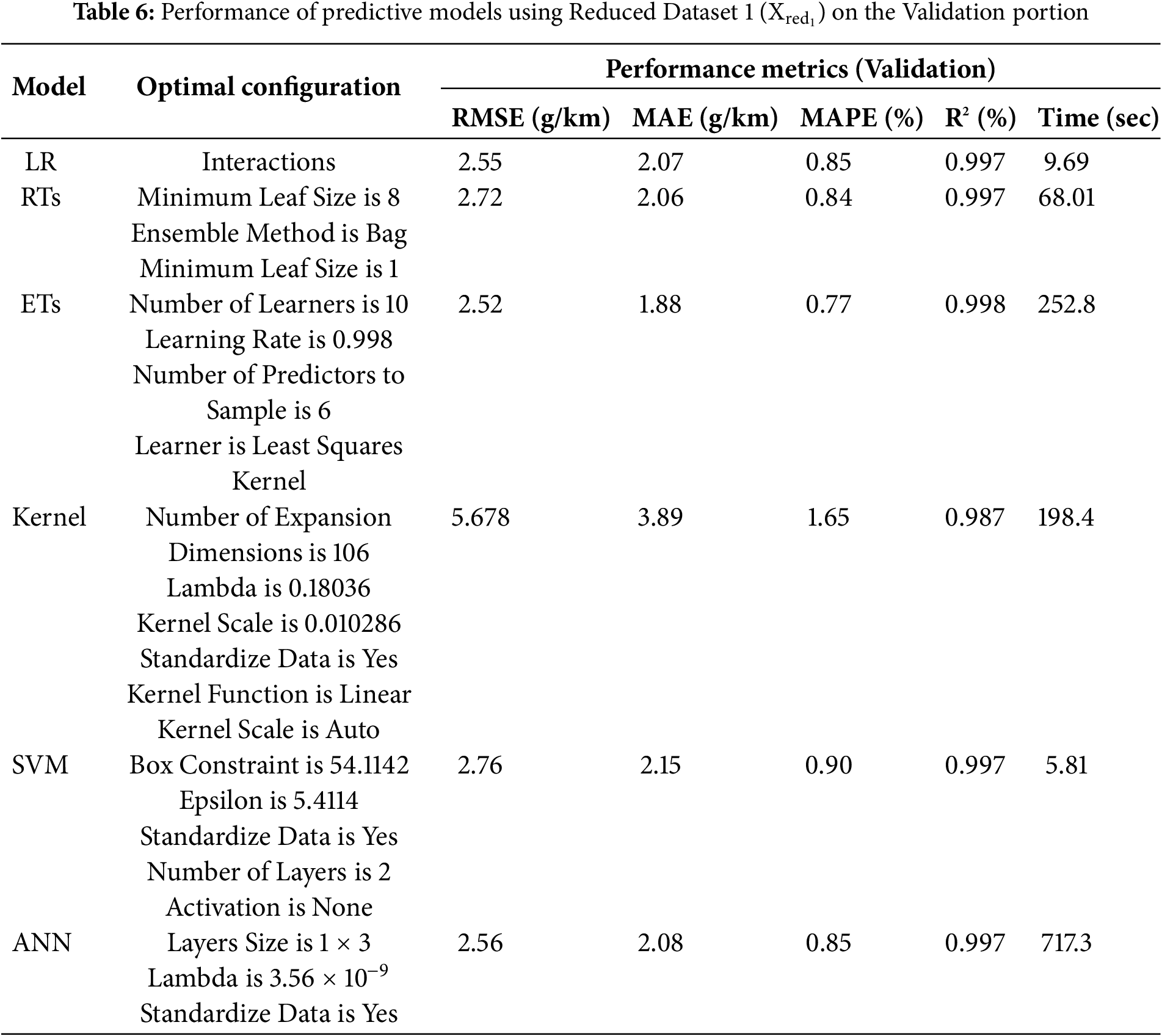
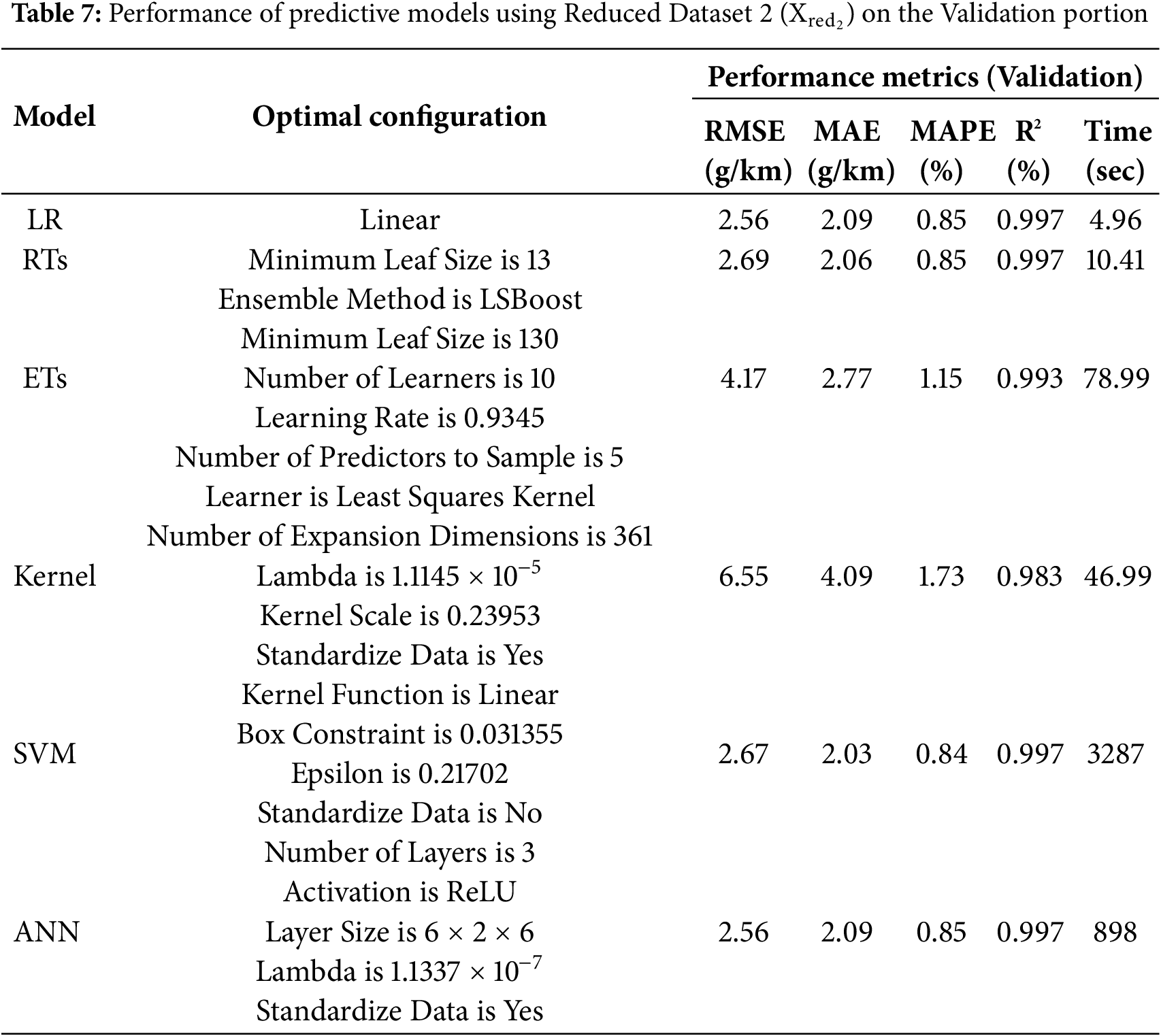
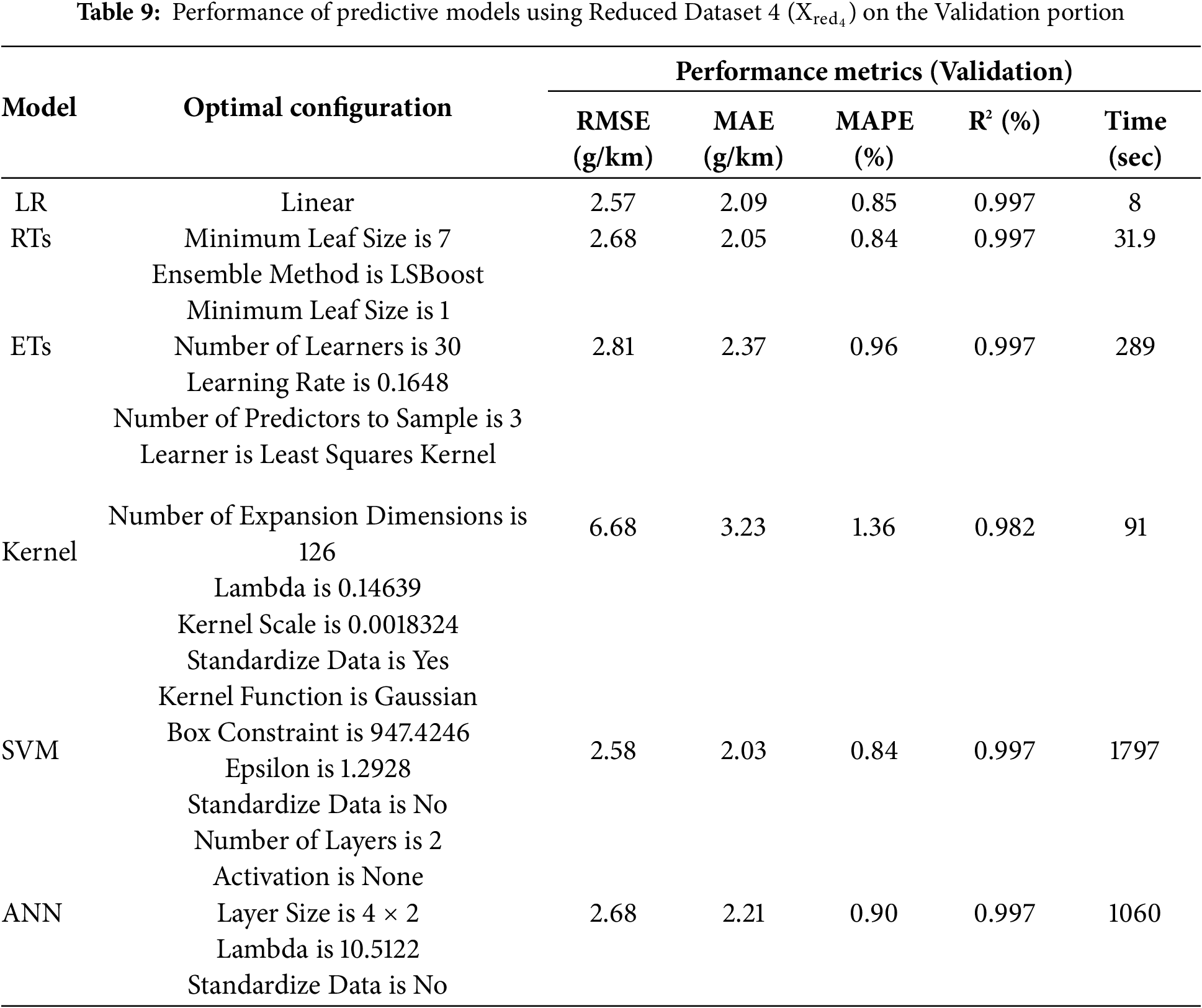
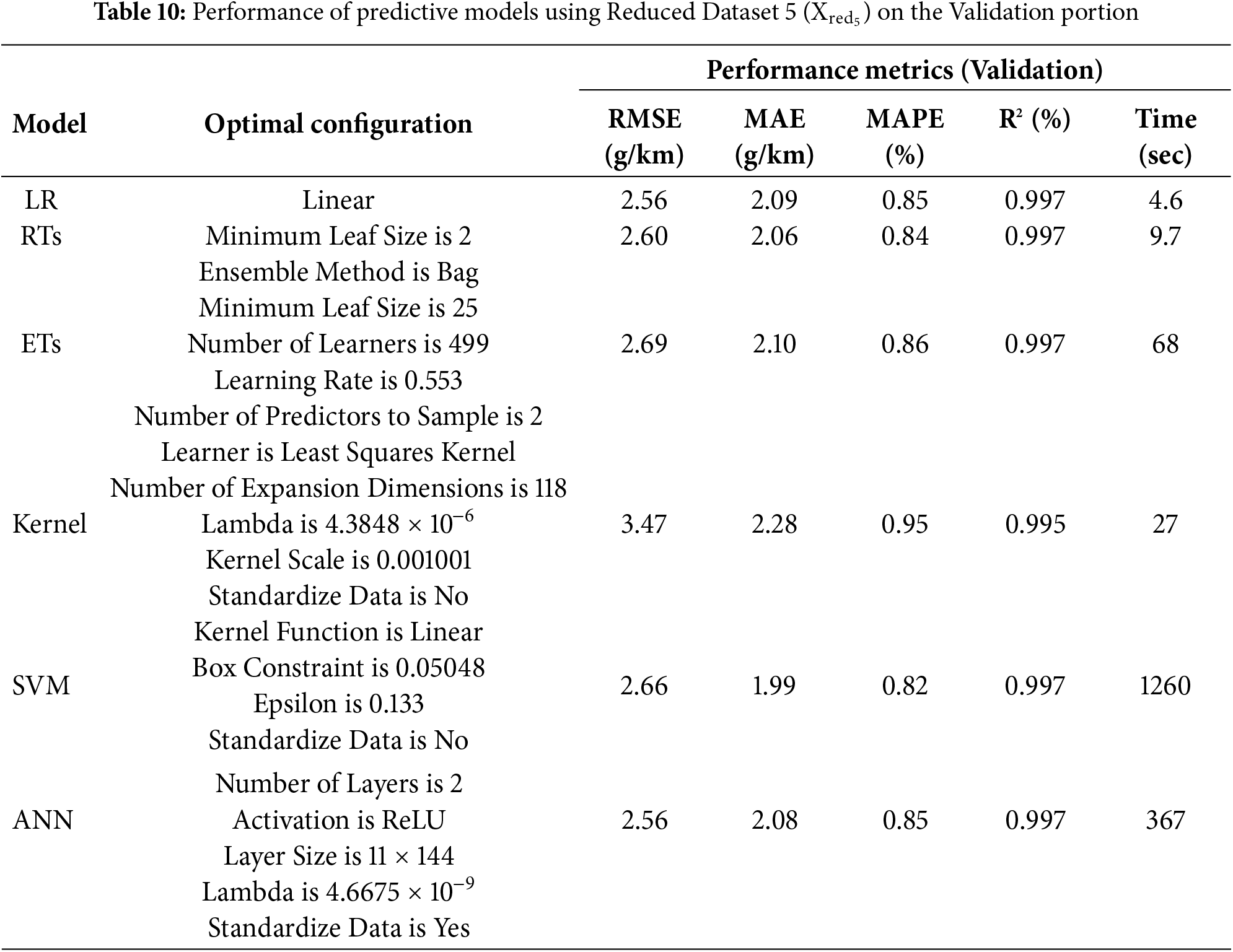
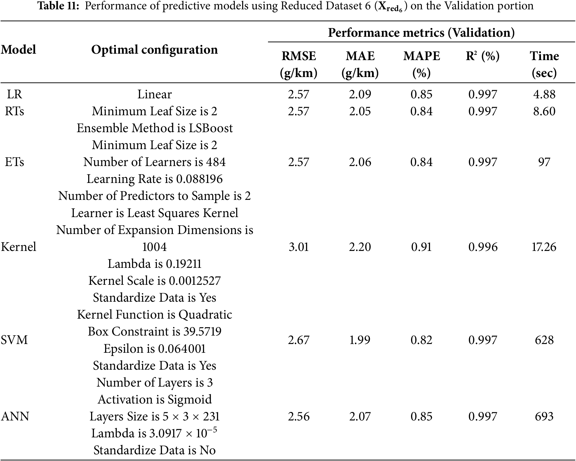
Looking at the tables, one can clearly observe that, across all performance metrics, reducing the number of attributes/features used to develop the prediction models (i.e., moving from Xred1 to Xred6) does not significantly impact prediction accuracy, except in the case of the Kernel model, where performance appears to deteriorate as the number of attributes decreases. This suggests that the removed attributes may not provide unique predictive information and are likely non-essential or redundant, with their effects already captured by the most influential attribute, i.e., Fuel Consumption. In fact, the use of a simple LR model may be sufficient, offering a favorable compromise between predictive accuracy and computational efficiency.

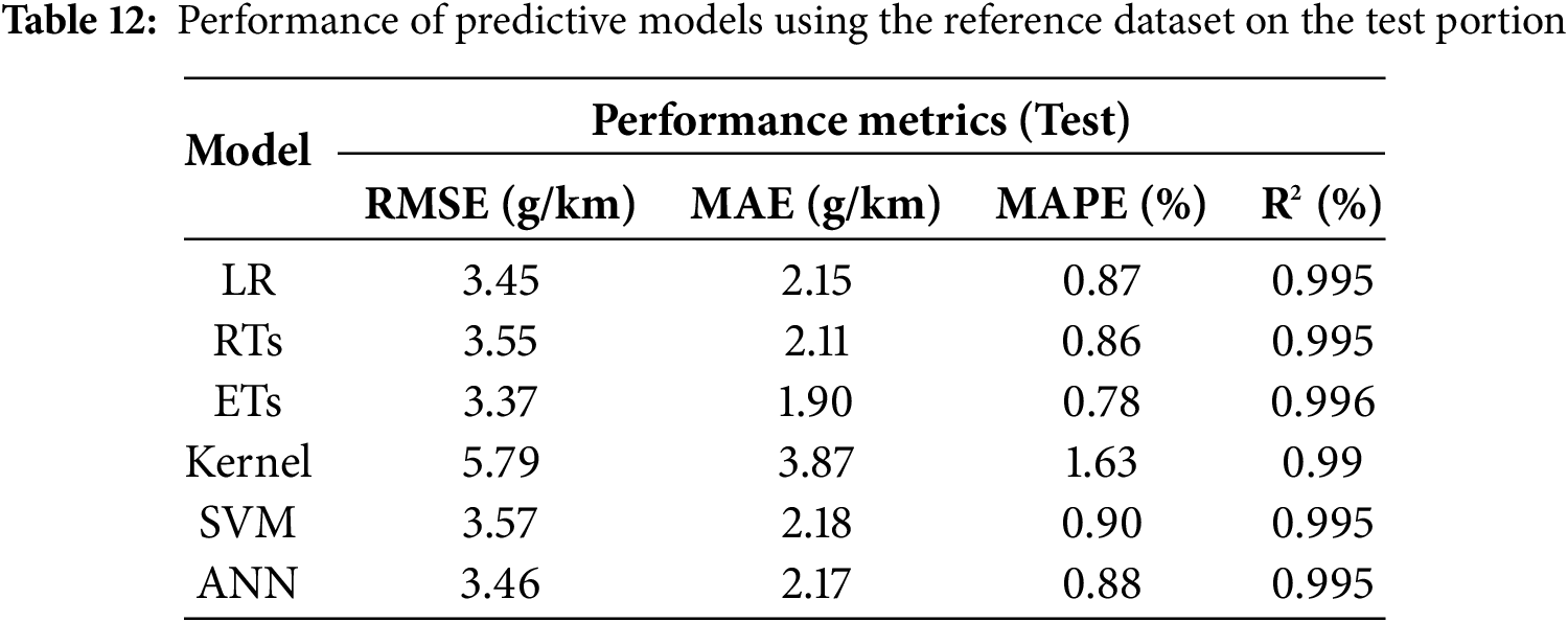
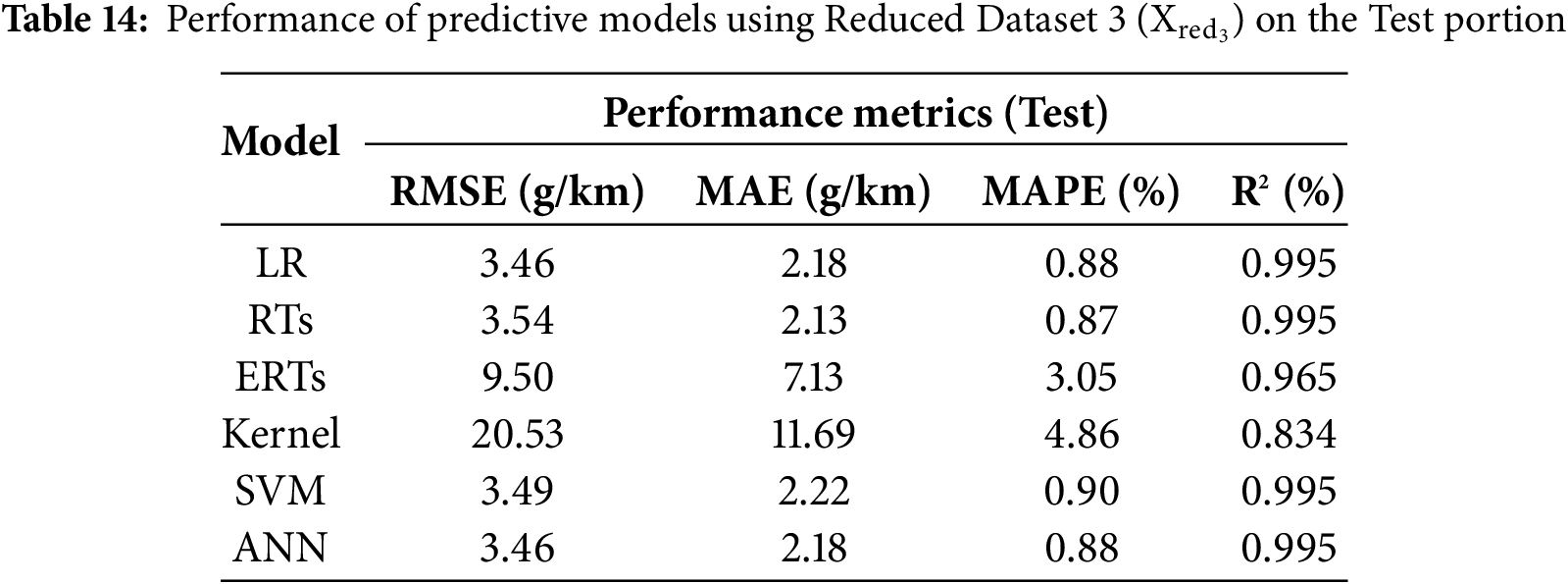
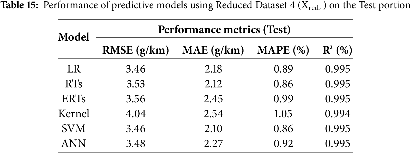
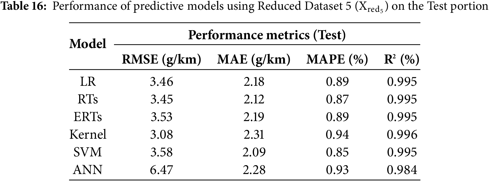
Once the optimal models are identified, they will be used to evaluate the predictability of the CO2 emissions on the 20% test portion. It is crucial to benchmark and compare the developed models under identical conditions, i.e., using the same test dataset with the same operating settings, to ensure a fair and meaningful assessment of their performance. In this regard, Tables 12–17 summarize the models’ performance across the dataset variants, reporting the achieved RMSE, MAE, MAPE, and R2 metrics’ values. Looking at the tables, one can observe that the models’ performance remains nearly consistent across all performance metrics, except for the Kernel model, whose performance varies between different dataset variants. Furthermore, the performance metrics align closely with those obtained on the validation set across all models, indicating that overfitting did not occur on the unseen test set.

For further clarity, Fig. 26 shows the actual (solid line) and predicted (solid lines with different markers) CO2 emissions obtained by the LR on the test portion across the dataset variants. An exact match can be observed among the estimates obtained while using the different dataset variants.

Figure 26: Examples of actual vs. predicted CO2 emissions obtained by the LR for 50 test vehicles across the dataset variants

To justify the performance of our models, a careful comparative study to two studies that used the same dataset was carried out. Based on the Bi-LSTM deep neural network, the performance metrics in terms of R2 on the testing 20% of the whole dataset was reported to be 93.78% [25]. Therefore, our models yield substantially better results than those of [25] since they yielded an R2 between 98% and 99% in the out-of-sample testing datasets. Similarly, the accuracy of the models investigated in [26] was found to be comparable to our study performance metrics with a superiority to our models since they are simpler and straightforward against the deep neural networks tested in [26] known to be time-consuming during their training phase.

The findings of our study have shown the proposed models to accurately predict the level of CO2 being emitted by the investigated LDVs. For instance, using machine learning techniques exhibited significant implications for both policy and industry applications. Policymakers can benefit from these predictive models to improve the effectiveness of the regulations and emission standards, ensuring compliance with environmental goals such as those stated in the Paris Agreement. In addition, the LDVs manufacturers can use the findings of this study (mainly the features that are the most likely to affect the CO2 emission levels) to lower the current levels. At the regional level, each country in which the investigated LDVs are used can inspire those insights to check the expected CO2 levels even before importing any type of the studied vehicles.

6  Conclusions, Limitations, and Future Directions

In this paper, the predictability of CO2 emissions from Light-Duty Vehicles (LDVs) was investigated using a comprehensive dataset encompassing LDVs from various manufacturers, their CO2 emissions, and other critical influencing attributes. Six Machine Learning (ML) models, ranging from simple linear regression models to highly non-linear regression models, were developed and optimized to estimate CO2 emissions accurately. To facilitate the models’ development stage, a detailed statistical analysis was conducted to identify the most influential attributes of CO2 emissions. Three correlation metrics, namely Pearson, Spearman, and Kendall, were employed to compute attribute correlations. Based on the computed correlation values, different reduced dataset variants were established to optimally identify the set of attributes that maximize the predictability of CO2 emissions. The effectiveness of the developed ML models was examined across these dataset variants using well-established performance metrics from the literature. The obtained results reveal that Fuel Consumption attributes were the most influential on CO2 emissions, as evidenced by their high correlation values across all three metrics. The investigated models demonstrated consistent performance across all metrics and dataset variants, with the LR model emerging as the optimal choice due to its balance between predictive accuracy and computational efficiency. Specifically, the LR model achieved superior performance, with the Mean Absolute Percentage Error falling below 0.90% and the Coefficient of Determination exceeding 99.7%. These results were obtained using the 80-20 rule for validation and test datasets, respectively, and a 5-fold cross validation approach on the validation dataset. While this work underscores the effectiveness of various ML models, particularly NNs, in accurately estimating CO2 emissions from LDVs, several limitations can be identified, along with recommendations to enhance the robustness and applicability of the findings:

-   The study relies solely on standalone ML models, which may limit predictive performance compared to hybrid approaches that leverage complementary strengths. Thus, future work can be devoted to exploring hybrid modeling approaches to further enhance prediction accuracy.

-   The dataset used in this study may not fully capture the variability of real-world driving conditions, as it lacks attributes such as speed variability, driving behavior, fuel quality, and road conditions. Thus, future work can be devoted to expanding the dataset by the inclusion of such additional attributes to provide a deeper understanding of the attributes influencing CO2 emissions and improve the models’ predictability.

-   The developed ML models were trained on a static dataset, making the models less adaptable to evolving conditions experienced by the vehicles over time. Thus, future work can be devoted to integrating incremental learning methods to allow models to effectively adapt to evolving conditions, ensuring their long-term applicability.

-   Inspired by the work presented in [23] which explored the ability of several statistical and ML models to forecast annual CO2 emissions of the building sector, the findings can be extended to the transportation sector to predict the quantity of CO2 expected to be emitted by the LDVs at a country level. To carry out such research, statistics of the vehicles being used over the past years as well as the distribution of their brands, manufacturers, average time of annual use, etc. are key information.

Acknowledgement: The authors extend their appreciation to the Deputyship for Research & Innovation, Ministry of Education in Saudi Arabia for funding this research work through the project number MoE-IF-UJ-R2-22-20772-1.

Funding Statement: Deputyship for Research & Innovation, Ministry of Education in Saudi Arabia, project number MoE-IF-UJ-R2-22-20772-1.

Author Contributions: The authors confirm their contribution to the paper as follows: Conceptualization, Sahbi Boubaker, Faisal S. Alsubaei and Sameer Al-Dahidi; Data curation, Sahbi Boubaker and Sameer Al-Dahidi; Formal analysis, Sahbi Boubaker; Funding acquisition, Sahbi Boubaker; Investigation, Faisal S. Alsubaei; Methodology, Sameer Al-Dahidi; Project administration, Sahbi Boubaker; Resources, Sahbi Boubaker and Sameer Al-Dahidi; Software, Sameer Al-Dahidi; Supervision, Sahbi Boubaker; Validation, Sahbi Boubaker and Faisal S. Alsubaei; Writing—original draft, Sameer Al-Dahidi and Sahbi Boubaker; Writing—review & editing, Faisal S. Alsubaei. All authors reviewed the results and approved the final version of the manuscript.

Availability of Data and Materials: The authors confirm that the data supporting the findings of this study are available online.

Ethics Approval: Not applicable.

Conflicts of Interest: The authors declare no conflicts of interest to report regarding the present study.

Appendix A

Figs. A1 and A2 show the Pearson and Spearman correlation heatmaps computed on the refined dataset, using the numeric and numeric and encoded categorical attributes, respectively.

Figure A1: Pearson correlation heatmap

Figure A2: Spearman correlation heatmap

1https://www.kaggle.com/datasets/debajyotipodder/co2-emission-by-vehicles (accessed on 03 June 2025)

2https://www.mathworks.com/help/stats/regression-learner-app.html (accessed on 03 June 2025)

References

1. Raymand F, Ahmadi P, Mashayekhi S. Evaluating a light duty vehicle fleet against climate change mitigation targets under different scenarios up to 2050 on a national level. Energy Policy. 2021;149(1):111942. doi:10.1016/j.enpol.2020.111942. [Google Scholar] [CrossRef]

2. Awan A, Alnour M, Jahanger A, Onwe JC. Do technological innovation and urbanization mitigate carbon dioxide emissions from the transport sector? Technology in Society. 2022;71:102128. doi:10.1016/j.techsoc.2022.102128. [Google Scholar] [CrossRef]

3. Fayyazbakhsh A, Bell ML, Zhu X, Mei X, Koutný M, Hajinajaf N, et al. Engine emissions with air pollutants and greenhouse gases and their control technologies. J Clean Prod. 2022;376(369):134260. doi:10.1016/j.jclepro.2022.134260. [Google Scholar] [CrossRef]

4. Li B, Geng Y, Xia X, Qiao D. The impact of government subsidies on the low-carbon supply chain based on carbon emission reduction level. Int J Environ Res Public Health. 2021;18(14):7603. doi:10.3390/ijerph18147603. [Google Scholar] [PubMed] [CrossRef]

5. Zhao P, Zeng L, Li P, Lu H, Hu H, Li C, et al. China’s transportation sector carbon dioxide emissions efficiency and its influencing factors based on the EBM DEA model with undesirable outputs and spatial Durbin model. Energy. 2022;238(3):121934. doi:10.1016/j.energy.2021.121934. [Google Scholar] [CrossRef]

6. Liu M, Zhang X, Zhang M, Feng Y, Liu Y, Wen J, et al. Influencing factors of carbon emissions in transportation industry based on CD function and LMDI decomposition model: China as an example. Environ Impact Assess Rev. 2021;90(1):106623. doi:10.1016/j.eiar.2021.106623. [Google Scholar] [CrossRef]

7. Kumari S, Singh SK. Machine learning-based time series models for effective CO2 emission prediction in India. Environ Sci Pollut Res. 2023;30(55):116601–16. doi:10.1007/s11356-022-21723-8. [Google Scholar] [PubMed] [CrossRef]

8. Adamiak B, Szczotka A, Woodburn J, Merkisz J. Comparison of exhaust emission results obtained from Portable Emissions Measurement System (PEMS) and a laboratory system. Combustion Engines. 2023;195(4):128–35. doi:10.19206/ce-172818. [Google Scholar] [CrossRef]

9. Zhou G, Mao L, Bao T, Zhuang F. Machine learning-driven CO2 emission forecasting for light-duty vehicles in China. Transp Res Part D: Transp Environ. 2024;137(21):104502. doi:10.1016/j.trd.2024.104502. [Google Scholar] [CrossRef]

10. Natarajan Y, Wadhwa G, Sri Preethaa KR, Paul A. Forecasting carbon dioxide emissions of light-duty vehicles with different machine learning algorithms. Electronics. 2023;12(10):2288. doi:10.3390/electronics12102288. [Google Scholar] [CrossRef]

11. Robaina M, Neves A. Complete decomposition analysis of CO2 emissions intensity in the transport sector in Europe. Res Transp Econ. 2021;90(5):101074. doi:10.1016/j.retrec.2021.101074. [Google Scholar] [CrossRef]

12. Çınarer G, Yeşilyurt MK, Ağbulut Ü, Yılbaşı Z, Kılıç K. Application of various machine learning algorithms in view of predicting the CO2 emissions in the transportation sector. Sci Technol Energy Transit. 2024;79(6):15. doi:10.2516/stet/2024014. [Google Scholar] [CrossRef]

13. Jia T, Zhang P, Chen B. A microscopic model of vehicle Co2 emissions based on deep learning—a spatiotemporal analysis of taxicabs in Wuhan, China. IEEE Trans Intell Transp Syst. 2022;23(10):18446–55. doi:10.1109/tits.2022.3151655. [Google Scholar] [CrossRef]

14. Tena-Gago D, Golcarenarenji G, Martinez-Alpiste I, Wang Q, Alcaraz-Calero JM. Machine-learning-based carbon dioxide concentration prediction for hybrid vehicles. Sensors. 2023;23(3):23–3. doi:10.3390/s23031350. [Google Scholar] [PubMed] [CrossRef]

15. Liu R, He HD, Zhang Z, Wu CL, Yang JM, Zhu XH, et al. Integrated MOVES model and machine learning method for prediction of CO2 and NO from light-duty gasoline vehicle. J Clean Prod. 2023;422(45):138612. doi:10.1016/j.jclepro.2023.138612. [Google Scholar] [CrossRef]

16. Udoh J, Lu J, Xu Q. Application of machine learning to predict CO2 emissions in light-duty vehicles. Sensors. 2024;24(24):8219. doi:10.3390/s24248219. [Google Scholar] [PubMed] [CrossRef]

17. Li X, Ren A, Li Q. Exploring patterns of transportation-related CO2 emissions using machine learning methods. Sustainability. 2022;14(8):4588. doi:10.3390/su14084588. [Google Scholar] [CrossRef]

18. Moon S, Lee J, Kim HJ, Kim JH, Park S. Study on CO2 emission assessment of heavy-duty and ultra-heavy-duty vehicles using machine learning. Int J Automot Technol. 2024;25(3):651–61. doi:10.1007/s12239-024-00051-5. [Google Scholar] [CrossRef]

19. Mądziel M. Instantaneous CO2 emission modelling for a Euro 6 start-stop vehicle based on portable emission measurement system data and artificial intelligence methods. Environ Sci Pollut Res. 2024;31(5):6944–59. doi:10.1007/s11356-023-31022-5. [Google Scholar] [PubMed] [CrossRef]

20. Zhong D, Liu X, Haroon M. Revolutionizing urban emission tracking: enhanced vehicle ratios via remote sensing techniques. Trans Res Part D: Trans Environ. 2024;137(2):104492. doi:10.1016/j.trd.2024.104492. [Google Scholar] [CrossRef]

21. Li S, Tong Z, Haroon M. Estimation of transport CO2 emissions using machine learning algorithm. Trans Res Part D: Trans Environ. 2024;133(6):104276. doi:10.1016/j.trd.2024.104276. [Google Scholar] [CrossRef]

22. Pearson K. Notes on regression and inheritance in the case of two parents. Proc R Soc Lond. 1895;58:240–2. [Google Scholar]

23. Spearman C. The proof and measurement of association between two things. Am J Psychol. 1987;3(4):441–71. [Google Scholar]

24. Kendall MG. A new measure of rank correlation. Vol. 30. Oxford, UK: Oxford University Press; 1938. p. 81–93. [Google Scholar]

25. Al-Nefaie AH, Aldhyani THH. Predicting CO2 emissions from traffic vehicles for sustainable and smart environment using a deep learning model. Sustainability. 2023;15(9):7615. doi:10.3390/su15097615. [Google Scholar] [CrossRef]

26. Gurcan F. Forecasting CO2 emissions of fuel vehicles for an ecological world using ensemble learning, machine learning, and deep learning models. PeerJ Comput Sci. 2024;10(9):e2234. doi:10.7717/peerj-cs.2234. [Google Scholar] [PubMed] [CrossRef]