
 Submit a Paper
 Propose a Special lssue
 Open Access
ARTICLE
Application and Performance Optimization of SLHS-TCN-XGBoost Model in Power Demand Forecasting
1 Department of Trade and Logistics, Daegu Catholic University, Gyeongsan, 38430, Republic of Korea
2 Digital Economy Research Institute, Chengdu Jincheng College, Chengdu, 611731, China
3 Department of Mathematics, Faculty of Science, Mahasarakham University, Maha Sarakham, 44150, Thailand
4 Institute of Seismology, China Earthquake Administration, Wuhan, 430071, China
5 The Digital Innovation Research Cluster for Integrated Disaster Management in the Watershed, Mahasarakham University, Maha Sarakham, 44150, Thailand
* Corresponding Author: Piyapatr Busababodhin. Email:
Computer Modeling in Engineering & Sciences 2025, 143(3), 2883-2917. https://doi.org/10.32604/cmes.2025.066442
Received 08 April 2025; Accepted 11 June 2025; Issue published 30 June 2025
 View Full Text
 Download PDF
Abstract
Existing power forecasting models struggle to simultaneously handle high-dimensional, noisy load data while capturing long-term dependencies. This critical limitation necessitates an integrated approach combining dimensionality reduction, temporal modeling, and robust prediction, especially for multi-day forecasting. A novel hybrid model, SLHS-TCN-XGBoost, is proposed for power demand forecasting, leveraging SLHS (dimensionality reduction), TCN (temporal feature learning), and XGBoost (ensemble prediction). Applied to the three-year electricity load dataset of Seoul, South Korea, the model’s MAE, RMSE, and MAPE reached 112.08, 148.39, and 2%, respectively, which are significantly reduced in MAE, RMSE, and MAPE by 87.37%, 87.35%, and 87.43% relative to the baseline XGBoost model. Performance validation across nine forecast days demonstrates superior accuracy, with MAPE as low as 0.35% and 0.21% on key dates. Statistical Significance tests confirm significant improvements (p < 0.05), with the highest MAPE reduction of 98.17% on critical days. Seasonal and temporal error analyses reveal stable performance, particularly in Quarter 3 and Quarter 4 (0.5%, 0.3%) and nighttime hours (<1%). Robustness tests, including 5-fold cross-validation and Various noise perturbations, confirm the model’s stability and resilience. The SLHS-TCN-XGBoost model offers an efficient and reliable solution for power demand forecasting, with future optimization potential in data preprocessing, algorithm integration, and interpretability.Keywords
Against the backdrop of the continuous growth of global energy demand, power demand forecasting, as the core of power system planning and operation, has become increasingly important. Accurate power demand forecasting can not only optimize the allocation of power resources but also improve the stability and economy of the power grid, thus providing strong support for the sustainable development of the energy industry. However, although traditional power demand forecasting methods, such as linear regression and ARIMA models, have dominated early research, their limitations have gradually emerged [1]. These methods mainly rely on the linear relationship of time series, and it is difficult to effectively process high-dimensional, nonlinear, and complex dynamic power demand data. Especially when facing large-scale data, the problems of high computational complexity and difficulty in feature selection are particularly prominent [2].
To overcome the aforementioned limitations, this study proposes a novel hybrid model—Sequential Latin hypercube sampling–Temporal Convolutional Network–eXtreme Gradient Boosting (SLHS–TCN–XGBoost)—which seamlessly integrates SLHS for feature dimensionality reduction, TCN for capturing temporal dependencies, and XGBoost for robust nonlinear regression. This integration aims to significantly improve both the accuracy and robustness of power demand forecasting [3]. This model aims to significantly improve the accuracy and robustness of power demand forecasting by combining the high-dimensional data processing capabilities of SLHS, the time series modeling capabilities of TCN, and the integrated learning advantages of XGBoost [4]. The SLHS model reduces redundant features through latent heatmap smoothing. This improves data representation while maintaining critical patterns; the TCN model captures long-term dependencies in the time series through dilated convolution and causal convolution structures, and XGBoost further optimizes the prediction results through the gradient boosting framework and regularization technology [5]. This innovative strategy of combining multiple models can not only effectively deal with the high dimensionality, noise, and complexity of power demand data but also provide an efficient and reliable solution for power demand forecasting.
The core goal of this study is to optimize the accuracy of power demand forecasting through the combination of the SLHS-TCN-XGBoost model and to solve the limitations of traditional methods in dealing with high-dimensional and nonlinear data. Specifically, this study aims to reduce the data dimension through the feature extraction capability of the SLHS model, capture the long-term dependency of power demand through the time series modeling capability of the TCN model, and further improve the stability and accuracy of the forecast results through the ensemble learning capability of XGBoost [6]. In addition, this study is also committed to solving the data noise problem in power demand forecasting and verifying the adaptability and reliability of the model under different data conditions through robustness testing and error analysis.
The main contribution of this paper is to propose an innovative hybrid model, SLHS-TCN-XGBoost, and verify its superior performance in power demand forecasting through a large number of experiments. The specific contributions include:
1. Innovative fusion of SLHS, TCN, and XGBoost: for the first time, the three technologies of SLHS, TCN, and XGBoost are organically combined to give full play to their respective advantages in feature extraction, time series modeling, and ensemble learning, and effectively improve the power demand forecasting task.
2. Significantly improve prediction accuracy and robustness: through a large number of experiments, it is proved that the SLHS-TCN-XGBoost model has significant advantages in prediction accuracy, robustness, and adaptability in power demand forecasting tasks, especially in processing high-dimensional and nonlinear data.
3. Verification of model stability and reliability: through cross-validation, noise testing and other experimental methods, the stability and reliability of the SLHS-TCN-XGBoost model under different data conditions are verified, providing solid technical support for the practical application of power demand forecasting.
4. Strengthen the adaptability to high-dimensional and complex data: SLHS technology effectively selects features and reduces dimensions, enabling TCN to better capture complex patterns in time series data, while XGBoost improves the prediction accuracy and robustness of the overall model through ensemble learning, and enhances the ability to process high-dimensional and complex data.
5. Promote the practical application of power demand forecasting: the SLHS-TCN-XGBoost model proposed in this study not only provides an efficient and reliable solution for the field of power demand forecasting but also provides strong support for further application in actual power systems, and has great practical application potential.
The structure of this paper is as follows: Section 2 reviews the relevant research on power demand forecasting, analyzes the limitations of traditional methods and machine learning methods, and introduces the advantages of technologies such as SLHS, TCN and XGBoost; Section 3 elaborates on the methodology of the SLHS-TCN-XGBoost model, including the design and application of the SLHS model, the training and optimization of the TCN model, the optimization of the XGBoost integrated algorithm, and the fusion and optimization strategy of the model; Section 4 introduces the experimental design and data analysis, including data sets and preprocessing, parameter settings, evaluation indicators, and comparative analysis of prediction models; Section 5 conducts an in-depth analysis of the experimental results, including statistical significance tests, robustness tests, error analysis, and sensitivity analysis; Section 7 summarizes the main conclusions of this study and proposes the direction of future research. Through systematic theoretical analysis and experimental verification, this paper provides an efficient and reliable solution for the field of power demand forecasting, which has important theoretical significance and practical application value.
Power demand forecasting is the key to power system planning and operation. Its accuracy directly affects the rational allocation of power resources and the stable operation of the power grid. Traditional statistical methods, such as linear regression and ARIMA models, dominated early research. These methods predict by capturing the linear relationship of time series, but have limited performance when dealing with nonlinear and high-dimensional data [7,8]. With the development of machine learning technology, methods such as Support Vector Machines (SVM), neural networks, and random forests have gradually been introduced into the field of power demand forecasting [9,10]. These methods can better handle nonlinear relationships, but when faced with large-scale and high-dimensional data, they still have problems such as high computational complexity and difficulty in feature selection. In recent years, deep learning methods such as Long Short-Term Memory network (LSTM) and Convolutional neural network (CNN) have shown significant advantages in power demand forecasting, especially in capturing the long-term dependency and spatial characteristics of time series [11,12]. However, deep learning methods also face challenges such as long training times and complex hyperparameter tuning.
As an emerging high-dimensional data processing method, the SLHS model has been widely used in power demand forecasting in recent years. The SLHS model can effectively reduce redundant features in the data by introducing latent heatmap smoothing technology, thereby improving the data representation ability [13]. Its core idea is to generate more representative latent features by reducing the dimension and extracting features from high-dimensional data, thereby improving the prediction accuracy. When processing power demand data, the SLHS model can effectively capture the seasonality, trend and randomness characteristics of the load, especially in high-dimensional and nonlinear data scenarios. In addition, the SLHS model has good interpretability and can provide strong support for the decision-making of the power system.
TCN is a time series modeling method based on CNNs. It can effectively capture long-term dependencies in time series through dilated convolution and causal convolution structures [14]. Compared with traditional Recurrent neural networks (RNNs), TCN has the advantages of strong parallel computing capabilities and high training efficiency. However, TCN still has certain limitations when dealing with complex nonlinear relationships. XGBoost is an efficient ensemble learning method that can effectively reduce the risk of overfitting of the model and improve prediction accuracy through the gradient boosting framework and regularization technology [15]. Combining TCN with XGBoost can give full play to the advantages of both: TCN is responsible for extracting the deep features of the time series, while XGBoost further optimizes the prediction results through ensemble learning. This fusion strategy can not only improve the prediction accuracy of the model but also enhance the model’s adaptability to complex power demand patterns [16].
In addition to the TCN-XGBoost model, ensemble methods have been extensively applied to power demand forecasting. Recent advances emphasize multi-stage frameworks, such as a decomposition-based ensemble model incorporating error factors and multi-objective optimization to enhance accuracy through residual error mitigation and feature interaction analysis [17]. Similarly, a hybrid ensemble learning approach with error correction has demonstrated robustness in short-term industrial load forecasting, particularly for volatile demand patterns [18]. The SLHS-SVM-AdaBoost model leverages SLHS for feature extraction, SVM for nonlinear mapping, and AdaBoost for ensemble learning, collectively improving predictive performance [19]. Further, SLHS-LSTM synergizes latent heatmap smoothing with LSTM to capture long-term temporal dependencies [20]. Hybrid architecture has also been advanced through integrating temporal pattern attention (TPA) with Bidirectional Long Short-Term Memory (BiLSTM) and optimized via chaos search sparrow algorithms (CSSA), achieving adaptive feature weighting and superior short-term forecasting results [21]. Spatial-temporal modeling is addressed by CNN-BiLSTM-Attention, where CNN extracts spatial features, BiLSTM processes bidirectional temporal dependencies, and attention mechanisms dynamically weight features [22]. The LSTM-XGBoost fusion combines sequential modeling with gradient-boosted ensemble learning, further refining prediction accuracy [23].
Although existing research has made significant progress in the field of power demand forecasting, there are still some shortcomings and challenges. Firstly, when processing high-dimensional and nonlinear data, existing models often require complex feature engineering and hyperparameter tuning, which increases the difficulty of model application [24]. Secondly, data preprocessing and feature selection have a great impact on model performance. How to design efficient data preprocessing processes and feature selection methods is still an urgent problem to be solved [25]. In addition, the optimization of model fusion strategy is also an important research direction. How to reduce model complexity while ensuring prediction accuracy is one of the key challenges for future research [26]. Finally, the actual application scenarios of power demand forecasting are complex and diverse. How to design a prediction model with strong versatility and wide adaptability still needs further exploration.
3 Methodology of the SLHS-TCN-XGBoost Model
3.1 Design and Application of the SLHS Model
As an efficient feature selection and dimensionality reduction method, the SLHS model has shown significant advantages in high-dimensional data processing. In the field of power demand forecasting, the SLHS model can extract the most representative features from massive power data and effectively eliminate redundant information, thereby significantly improving the training efficiency and prediction accuracy of subsequent models. Its core goal is to reduce the dimension of feature space while retaining the key features of data by constructing a sparse subspace, thereby simplifying the computational complexity of the model and enhancing its generalization ability [27]. Fig. 1 shows the framework design of the SLHS model in time series forecasting, which is optimized specifically for power demand forecasting problems.
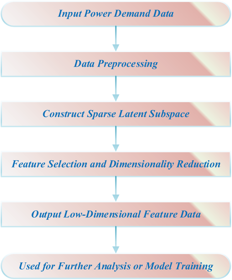
Figure 1: Framework of the SLHS model for time series forecasting
In power demand forecasting, the input power demand data first undergoes a series of rigorous data preprocessing steps, including noise filtering, missing value filling, and data standardization, to ensure the quality and consistency of the data, thereby providing a reliable basis for subsequent analysis and modeling. Subsequently, by constructing an SLHS, the model can extract key potential patterns and trends from complex power demand data. The core of this process is to use feature selection and dimensionality reduction techniques to effectively eliminate redundant and irrelevant features, thereby significantly improving the computational efficiency and prediction accuracy of the model. Finally, the model outputs optimized low-dimensional feature data, which not only retains the core information of power demand but also provides high-quality input for further analysis or model training.
Specifically, in power demand forecasting, SLHS first converts multidimensional time series data into a high-dimensional feature space by preprocessing historical power load data, and then uses a sparsification method to extract the most informative feature subsets in the data [28]. The power demand data set is
where
In the preprocessing of power demand data, SLHS can effectively transform the data into a low-dimensional space suitable for further processing through feature selection and dimensionality reduction methods. This process not only improves the training speed of subsequent models but also increases the sensitivity of the model to changes in power demand, thereby enhancing the prediction accuracy.
3.2 Training and Optimization of the TCN Model
In power demand forecasting, the training and optimization of the TCN model play a vital role. As a time series modeling method based on CNN, TCN can effectively process long-term data and perform deep learning of time series features through convolutional layers to extract potential time series patterns in power demand data. When processing time series data, the TCN model has stronger long-term memory ability than the traditional RNN, and the convolution structure can be calculated in parallel, which greatly improves the computational efficiency [29]. In the SLHS-TCN-XGBoost model framework, the TCN model further extracts richer time series features by training the power demand data after smoothing by the SLHS model, providing high-quality feature input for the subsequent XGBoost model. Fig. 2 shows the architecture of the TCN for time series analysis. The model processes the input time series data layer by layer through multiple convolutional layers.
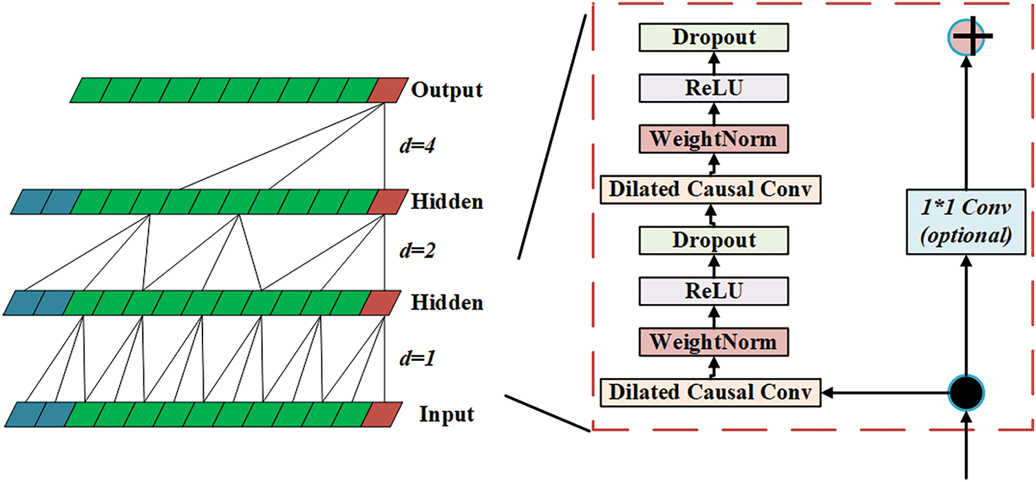
Figure 2: Time series analysis architecture of TCN
The training process of the TCN model first involves convolution operations on time series data. Unlike traditional CNNs, TCN uses a dilated convolution structure, which enables the model to capture long-distance dependencies in the convolution kernel in a jumpy manner, thereby overcoming the information loss problem of traditional CNNs when processing long time series [30]. The key to dilated convolution is to introduce a dilation factor
Among them,
In the optimization process of the TCN model, the training goal is to adjust the parameters of the model by minimizing the loss function. Common loss functions include the Mean square error (MSE) loss function, which can effectively measure the difference between the predicted value and the true value [34]. The true value of the power demand forecast is
During the training process, the loss function is minimized through the gradient descent algorithm to obtain the optimal parameters of the TCN model. The Adam optimizer dynamically adjusts the learning rate of each parameter by calculating the mean and variance of the gradient, greatly improving the stability and convergence speed of the training.
In addition, in order to avoid overfitting, the TCN model uses dropout and L2 regularization during the training process. Dropout prevents the model from overfitting the training data by randomly discarding some neurons in the neural network, while L2 regularization limits the size of the model weight by increasing the penalty term of the parameter, thereby further improving the generalization ability of the model [35].
3.3 Optimization of XGBoost Ensemble Algorithm
XGBoost is an ensemble learning method based on gradient boosting trees, which is widely used in efficient regression and classification. In the problem of power demand forecasting, the XGBoost model can improve the accuracy and robustness of the forecast by integrating the forecast results of multiple decision trees. The algorithm continuously optimizes the objective function so that the model can build an efficient forecast model based on the characteristics of the training data [36]. In the SLHS-TCN-XGBoost model, the role of XGBoost is mainly reflected in modeling the time series features extracted by the TCN model and generating the final power demand forecast results. Fig. 3 shows the forecast analysis architecture of the XGBoost model, which adopts the idea of the additive model, in which predictions are made by combining multiple decision trees. The input data is processed by each tree, and each node is weighted and calculated by weight parameters (such as

Figure 3: Prediction analysis architecture of XGBoost model
The optimization goal of XGBoost is to gradually build a series of weak classifiers (decision trees) through the gradient boosting algorithm and combine them into a strong classifier by weighted averaging. Specifically, XGBoost optimizes model parameters by minimizing the loss function. The common loss function is the MSE, which is expressed in the regression problem as:
Among them,
Through regularization, pruning, learning rate adjustment, and cross-validation, XGBoost can build an efficient prediction model with strong generalization ability. In the SLHS-TCN-XGBoost framework, XGBoost significantly improves the accuracy and stability of power demand forecasting by efficiently modeling the time series features extracted by TCN, providing reliable technical support for demand forecasting in the power industry.
3.4 Fusion and Optimization Strategy of SLHS-TCN-XGBoost Model
The fusion and optimization strategy of the SLHS-TCN-XGBoost model is the core to achieve high-precision prediction. This model combines three technologies: SLHS, TCN, and XGBoost. Through layer-by-layer deep learning and feature optimization, it effectively improves the modeling ability of complex time series data. The SLHS model provides stable input features for the TCN model through data preprocessing; then, the TCN model further extracts time series features through deep convolution learning, and sends these features to XGBoost for final prediction [38]. In order to further optimize the performance of the model, the prediction accuracy of the model can be improved by adjusting hyperparameters such as the expansion factor and convolution kernel size in the TCN model and the depth and learning rate of the tree in the XGBoost model. In practical applications, cross-validation technology is used to optimize hyperparameters, and the effects of different parameter combinations are evaluated through multiple experiments to select the optimal parameter configuration. Fig. 4 shows the combined framework of the SLHS-TCN-XGBoost model in power load forecasting. This framework combines the SLHS, the TCN and the XGBoost model to effectively improve the accuracy and stability of power load forecasting.

Figure 4: SLHS-TCN-XGBoost model combined framework in power load forecasting
At the input layer, historical power load data, weather data, and other related data are collected and passed to the entire framework. The data is preprocessed, including data cleaning, standardization, and missing value filling operations to ensure data quality and consistency. Then, the SLHS model constructs a sparse latent subspace, performs feature selection and dimensionality reduction, and outputs low-dimensional feature data. This process can effectively remove redundant information and extract features that are critical to power load forecasting.
These processed data then enter the TCN model. In the TCN model, data is processed through multi-layer convolution operations, and dilated causal convolution is used to capture long-term dependencies, helping the model to identify complex time series patterns in power loads. TCN can effectively identify nonlinear relationships in data through deep learning technology and prevent overfitting through Rectified Linear Unit activation functions and Dropout layers to improve the generalization ability of the model. The data processed by the TCN model is passed to the XGBoost model [39]. As an integrated learning method, XGBoost adopts a weighted fusion strategy in the process of model fusion. By calculating the weighted average of the prediction results of each module, the stability and accuracy of the prediction can be further improved. The equation for weighted fusion can be expressed as:
Among them,
In summary, the fusion and optimization strategy of the SLHS-TCN-XGBoost model forms a powerful prediction framework by combining a variety of advanced time series modeling techniques. Through data preprocessing, feature extraction, model training, and fusion strategies, the SLHS-TCN-XGBoost model can show excellent performance in power demand forecasting, with strong generalization ability and robustness. This model can not only effectively cope with the nonlinearity, time-varying, and complexity of power demand, but also provide reliable technical support for practical applications.
4 Experimental Design and Data Analysis
This study uses a power demand dataset from Seoul, South Korea, which covers hourly power load records for the past three years. The dataset has a total of 36 months of time series, a total of 78,912 data, including date, time, temperature, and power demand characteristics. Since the dataset is large and contains missing values, outliers, and multidimensional features, strict data preprocessing is required before model training. The identification of outliers is performed by calculating the data points with a single-day increase or decrease of more than 3 times the standard deviation, accounting for about 0.05% of the dataset. These outliers are caused by extreme market fluctuations or data entry errors. For missing values, interpolation is used to fill the missing values. For missing values in time series data, we use a combination of forward filling and linear interpolation to ensure data integrity. Fig. 5 shows the changing relationship between the average power demand and average temperature per month from January 2022 to December 2024. It can be clearly seen that power demand and temperature show a high seasonal correlation. As temperatures rise, especially in the summer, electricity demand increases significantly, while in the winter, when temperatures are lower, electricity demand is relatively low.

Figure 5: Average monthly electricity demand and temperature from 2022 to 2024
In summer months such as June 2022, June 2023, and June 2024, electricity demand approached or exceeded 7000 MW, while the average temperature rose to nearly 80°F, reflecting the driving effect of factors such as increased air conditioning use on electricity demand. In winter months such as December 2022 and December 2023, although the temperature dropped to nearly 30°F, electricity demand dropped to around 4500 MW. The overall trend shows the direct impact of temperature on electricity demand, especially when the seasons change, the temperature change significantly mobilizes the load fluctuation of the power system, showing a typical positive correlation between temperature and electricity demand.
For the division of the data set, we first use a data division ratio of 70%:15%:15% for model training. This ratio makes the training set data sufficient to ensure that the model obtains enough information during training, and the ratio of the validation set and the test set is sufficient for effective tuning and evaluation. However, using a data partition ratio of 80%:10%:10% or 60%:20%:20% will have different effects on model performance. To further analyze the potential impact of these partition ratios on performance, we will discuss two new partition ratios: 80%:10%:10% and 60%:20%:20%. We experimentally compare the performance of the SLHS-TCN-XGBoost model under different data partition ratios. Table 1 below lists the performance indicators under different data partition ratios, including MSE, Root mean square error (RMSE), Mean absolute error (MAE), Coefficient of determination (R2), and Mean absolute percentage error (MAPE).

According to the experimental results, the data partition ratio of 80%:10%:10% significantly improves the performance of the SLHS-TCN-XGBoost model, especially in terms of MSE, RMSE, and MAPE. This proves that more training data can help the model better learn the rules of power load data, thereby improving the prediction accuracy. In contrast, the partition ratio of 60%:20%:20% has less training data, which causes the model to fail to fully learn the patterns in the data, thereby reducing performance. Therefore, the data partition ratio of 80%:10%:10% is the best choice for this study, which can effectively improve the performance and generalization ability of the model.
4.2 Parameter Setting and Computing Resource Requirements
For the SLHS-TCN-XGBoost hybrid model proposed in this paper, considering that each submodule (SLHS, TCN, and XGBoost) has its independent hyperparameter requirements and needs to optimize the overall performance when integrated, we designed a systematic hyperparameter tuning process. First, the SLHS module dynamically determines the feature dimension reduction ratio by maximizing the correlation between features and target variables and minimizing the redundancy between features. Subsequently, the TCN module systematically searches within the range of key hyperparameters such as convolution kernel size, number of layers, and learning rate through the grid search method, and selects the optimal configuration based on the performance indicators of the validation set. The XGBoost module adjusts parameters such as learning rate, tree depth, and subsample ratio through cross-validation based on the RMSE performance of the validation set, thereby suppressing model complexity and improving generalization ability. In the overall tuning process of the hybrid model, we did not optimize the parameters of a single module separately, but sought the synergistic optimality among feature selection, time series modeling, and nonlinear regression based on end-to-end comprehensive performance evaluation to ensure that the outputs of each submodule can complement each other instead of interfering with each other. The entire tuning process combines grid search with empirical tuning, and the final parameters are determined through 5-fold cross-validation. The following are the hyperparameter configurations of each model and their corresponding computing resource requirements.
The learning rate of the XGBoost model is 0.05, the maximum depth of the tree is 6, the subsample ratio of 0.8, and the regularization parameter of 0.01 to avoid overfitting and improve the generalization ability of the model. In the TCN model, the Adam optimizer is used with a learning rate of 0.001, a batch size of 32, and a convolution kernel size of 3 to improve the training effect of the model and capture local features in time series data. The LSTM part uses a learning rate of 0.001 and 100 LSTM units, and the learning rate of the XGBoost part is 0.05, and the maximum depth of the tree is 6. The combination of LSTM and XGBoost can capture both time dependence and nonlinear relationships.
TCN uses a learning rate of 0.001 and a batch size of 64. The XGBoost part is the same as LSTM-XGBoost, with a learning rate of 0.05 and a maximum tree depth of 6. This combination improves the model’s ability to model temporal and nonlinear relationships. The CNN-BiLSTM-Attention model uses 3 convolutional layers and 128 BiLSTM units, combined with the Attention mechanism to improve prediction accuracy. The learning rate is 0.001, the batch size is 64, and the number of training rounds is 100. The SLHS-LSTM model uses SLHS for feature selection, and the LSTM part uses a learning rate of 0.01 and 128 units. The batch size is 64, and the number of training rounds is 100, which can effectively capture long-term dependencies.
The SLHS-SVM-AdaBoost model uses the Adam optimizer with a learning rate of 0.01, a batch size of 64, a training round of 100, a decay rate of 0.96, and a regularization parameter of 0.001, combining SVM and AdaBoost to improve prediction capabilities. The SLHS-TCN-XGBoost model combines SLHS for feature selection, TCN for time series modeling, and XGBoost for nonlinear modeling. The learning rate of TCN is 0.01, the convolution kernel size is 3, the learning rate of XGBoost is 0.05, and the maximum depth of the tree is 6. This combination improves the overall performance of the model.
All models in this study, especially deep learning and ensemble learning models such as TCN, LSTM, and XGBoost, have high requirements for computing resources during training. Especially when the amount of data is large, model training will take up a lot of CPU and GPU resources. To ensure efficient training and reasoning, the hardware configuration used in this article is NVIDIA RTX 4090 GPU; Intel® Core™ i9-14900KF processor (36 MB cache, up to 6.00 GHz); 5 TB memory.
To assess the practical feasibility of the proposed SLHS-TCN-XGBoost and other benchmark models, we measured the average and maximum training time per epoch, average and maximum inference time per sample, and peak GPU memory usage for each model. These evaluations were conducted under identical hardware conditions, using 10 independent runs to ensure stability. The results are summarized in Table 2.

In order to comprehensively evaluate the performance of the model in power load forecasting, we use a variety of evaluation indicators, covering aspects such as prediction accuracy, error distribution, and computational efficiency [40]. The specific evaluation indicators are as follows:
RMSE is the square root of MSE and is used to evaluate the magnitude of the prediction error. The equation is as follows:
The smaller the RMSE value, the more accurate the model prediction.
MAPE measures the error percentage of the model’s predicted value relative to the true value and is suitable for evaluating the error of the model in practical applications. The equation is as follows:
The smaller the MAPE value, the higher the prediction accuracy of the model.
MAE measures the average absolute difference between the model’s predicted value and the true value. It can intuitively reflect the size of the error and is not affected by outliers. The smaller the MAE value, the more accurate the model’s prediction. The equation is as follows:
Among them,
4.4 Comparison of Prediction Models
After the model training is completed, the features in the test set are input into multiple models to evaluate the model. In addition to the method used in this paper, seven models, including XGBoost, TCN, LSTM-XGBoost, TCN-XGBoost, CNN-BiLSTM-Attention, SLHS-LSTM, and SLHS-SVM-AdaBoost, are selected as comparison models. Fig. 6 shows the performance of different prediction models in power load prediction. The comparison between the actual value and the prediction results of various models is shown through time series, covering the prediction accuracy of various algorithms.

Figure 6: Time series comparison of actual and predicted values of power load by different prediction models
The prediction results of each model have certain errors in most time periods, especially in the peak period of power load, where the errors are more obvious. Specifically, the SLHS-TCN-XGBoost model shows lower errors than other models, the predicted values are closer to the actual values, and the volatility is smaller, which reflects the advantages of the model in dealing with high-frequency fluctuations. Its small error reflects that the model can better capture the load change trend and law in the long-term prediction of time series, reducing the possibility of overfitting.
For other models, although they can effectively track the change trend of power load in some time intervals, the error margin is relatively large when predicting peak and trough values. There are obvious deviations in the prediction results of LSTM-XGBoost and TCN models in certain periods, especially when the load demand fluctuates violently, the model fails to accurately capture the details of the load change, resulting in large prediction errors.
Overall, the prediction accuracy of each model can be further evaluated by quantitative indicators such as RMSE and MAPE. In terms of RMSE and MAPE values, the SLHS-TCN-XGBoost model showed the smallest error, indicating that its prediction ability in the entire period is superior to other models. Although the performance of other models varies, the overall error is relatively concentrated, and the prediction error of most models is more significant during peak periods, indicating that these models still have certain limitations when facing the volatility and complexity of power load forecasting.
Table 3 lists the main error indicators of different models in the power load forecasting task, including MAE, RMSE, and MAPE. As can be seen from the table, there are obvious differences in the prediction accuracy of each model, which is closely related to the model’s feature extraction ability, time series modeling depth, and overall architecture complexity.

Based on the three indicators of MAE, RMSE, and MAPE, the SLHS-TCN-XGBoost model performs best among all the compared methods, reaching 112.08, 148.39, and 2%, respectively. This shows that the model not only has a small overall error margin (low MAE and RMSE) in actual load forecasting but also has good prediction relative error control (low MAPE), and has the ability to cope with complex load fluctuations. In comparison, the performance of the SLHS-SVM-AdaBoost and SLHS-LSTM models is second, with MAE of 222.05 and 333.71, RMSE of 294.03 and 439.10, and MAPE of 3.98% and 5.99%, respectively. Although they have gaps with SLHS-TCN-XGBoost in various indicators, they can still maintain a relatively robust prediction effect within a certain range. Other benchmark models (CNN-BiLSTM-Attention, TCN-XGBoost, LSTM-XGBoost, TCN, and XGBoost) show larger error margins in all error indicators, verifying the effectiveness of feature selection and integration methods in improving power load forecasting performance.
Considering that the load change patterns in different seasons are different, the load curves on weekdays and weekends are also different. Different seasons, weekdays, and weekends in the data set are randomly selected, totaling 9 days as prediction days. Finally, 15 March (spring, working day), 25 June (summer, rest day), and 10 November (autumn, working day) in 2022 were selected. 20 January (winter, working day), 14 May (spring, rest day), and 05 September (autumn, working day) in 2023. 18 February (winter, rest day), 10 July (summer, working day), and 25 October (autumn, working day) in 2024 were selected as the forecast days. Fig. 7 shows the power load forecast results for 9 different forecast days, covering the load change rules in different seasons, working days, and rest days.

Figure 7: Power load forecast results for different seasons and working days/holidays
As can be seen from Fig. 7, the SLHS-TCN-XGBoost model has the best prediction effect on all selected dates. Whether on working days or holidays, the deviation between the model prediction value and the actual load is small, showing strong stability and accuracy. Especially in the period when the power load fluctuates greatly, SLHS-TCN-XGBoost can still track the changes in the actual load well, and the error is significantly lower than other models. Other models such as SLHS-SVM-AdaBoost, SLHS-LSTM, and CNN-BiLSTM-Attention also give relatively accurate predictions in most time periods, but their prediction results are poor during periods of drastic load fluctuations, especially during peaks and troughs. Table 4 shows the average prediction results of different models on 9 forecast days, including power load forecasts for ltiple seasons and working days and holidays in 2022 and 2023. By comparing the predicted values of each model with the actual values, the prediction ability of the model in different time periods and its performance in adapting to seasonal changes can be effectively evaluated.

From the data in Table 4, the SLHS-TCN-XGBoost model shows relatively stable prediction accuracy in all prediction days, and the average prediction error is relatively small. The prediction value of the model is close to the actual value, and the error level is kept at a low level within the fluctuation range of each date. In particular, on 15 March 2022 (spring, working day) and 14 May 2023 (spring, rest day), two relatively stable load periods, the prediction values of SLHS-TCN-XGBoost are 4203.72 and 4324.53, respectively, which are close to the actual values of 4188.88 and 4317.44, with small errors, reflecting its adaptability under different load fluctuations.
Other models, such as XGBoost, TCN, and LSTM-XGBoost, are slightly insufficient on some prediction days, especially on dates with large load fluctuations, such as 18 February 2024 (winter, rest day) and 05 September 2023 (autumn, working day), where the errors are large. The predicted value of XGBoost on 18 February 2024, is 5554.38, while the actual value is 5722.54, which has a certain deviation, showing the limitations of the model in dealing with seasonal changes and load fluctuations. The performance of TCN and LSTM-XGBoost is also affected to a certain extent by these factors, especially on 05 September 2023 (autumn, weekday) and 10 July 2024 (summer, weekday), where the errors are significantly increased, 4618.97 and 4420.90, respectively, while the actual values are 4330.28 and 4317.44.
Table 5 shows the RMSE of different models on 9 typical forecast days. By comparing the RMSE values of each model on different dates, its error level and prediction accuracy in handling load forecasting can be evaluated.

SLHS-SVM-AdaBoost and SLHS-TCN-XGBoost have low RMSE values on multiple dates, showing high prediction accuracy and good adaptability. Although other models, such as LSTM-XGBoost and TCN, perform well on certain dates, overall, their prediction errors fluctuate greatly. Therefore, the SLHS-SVM-AdaBoost and SLHS-TCN-XGBoost models perform better in power load forecasting, especially in different seasons and load fluctuation environments, showing strong stability and accuracy.
Table 6 lists the MAPE of different models on 9 typical forecast days. SLHS-SVM-AdaBoost shows extremely low MAPE on all dates, especially on 15 March 2022, and 25 June 2022, which are 0.13% and 0.07%, respectively, showing the excellent prediction accuracy of the model. SLHS-TCN-XGBoost also performs stably, and its MAPE values are generally low, especially on 14 May 2023, and 09 March 2024, which are 0.16% and 0.5%, respectively, highlighting the adaptability of the model to different load demands.

Table 7 shows the MAPE reduction values of different models on nine typical forecast days. SLHS-SVM-AdaBoost and SLHS-TCN-XGBoost showed significant MAPE reduction on most dates. In cases where the model performance was worse than the baseline, the reduction rate was set to zero to maintain mathematical consistency, especially on 15 March 2022, and 25 June 2022, reaching 97.63% and 99.16%, respectively, indicating that the prediction accuracy of these models on these dates has been significantly improved. SLHS-TCN-XGBoost also performed stably, with high MAPE reduction values on multiple dates, especially on 14 May 2023, and 25 October 2024, reaching 98.17% and 89.73%, respectively, indicating that the model’s prediction error on these dates has been significantly reduced.

5.1 Statistical Significance Test
In power demand forecasting, the SLHS-TCN-XGBoost model performs significantly better than the traditional model. In order to verify the statistical significance of its performance difference, we conducted a variety of statistical tests, including a t-test and a Post-hoc test. These tests not only helped us confirm the superiority of the model but also provided a scientific basis for further optimization [41].
We compared the differences between SLHS-TCN-XGBoost and XGBoost in RMSE and MAPE through a
Among them,

In the comparison of RMSE and MAPE, SLHS-TCN-XGBoost showed the lowest error values, 148.39 and 2%, respectively. Compared with XGBoost (RMSE 1172.85, MAPE 15.91%), the RMSE and MAPE values of SLHS-TCN-XGBoost were reduced by about 85% and 87%, respectively, and the results of the t-test showed that the p value was less than 0.05, indicating that the difference was significant. In comparison with other models, SLHS-TCN-XGBoost still performs significantly better than TCN, LSTM-XGBoost, and CNN-BiLSTM-Attention models. The statistically significant differences in RMSE and MAPE are both shown as large t values and p values less than 0.05, further verifying the superiority of this model in power demand forecasting. Other models, such as SLHS-SVM-AdaBoost (RMSE 294.03, MAPE 3.98%) and SLHS-LSTM (RMSE 439.10, MAPE 5.99%), also perform significantly better than XGBoost, but there is still a certain gap compared with SLHS-TCN-XGBoost.
The performance distribution of different models in terms of RMSE and MAPE is shown in Fig. 8 below.

Figure 8: Performance distribution of root MAE and MAPE across different forecasting models
The RMSE graph on the left shows that the XGBoost model has the smallest error and is significantly better than other models, especially in most cases, its error distribution is concentrated in the lower range. The TCN model is second, although there are some outliers, but the overall performance is relatively stable. Combination models such as LSTM-XGBoost and TCN-XGBoost show similar error distributions and are significantly higher than XGBoost. The MAPE graph on the right highlights the differences in prediction deviation rates among the models. XGBoost once again shows the best performance, with MAPE values generally below 20%, while other models are mostly concentrated in the higher MAPE range, especially SLHS-SVM-XGBoost, whose MAPE fluctuates greatly and has a higher mean. These results show that XGBoost shows strong robustness in both RMSE and MAPE indicators, while other more complex combination models fail to surpass the single model XGBoost in all indicators.
We further conducted a Post-hoc test to determine which specific models differed from each other. We used the Tukey HSD test, and its equation is as follows:
Among them,

The SLHS-TCN-XGBoost model shows a significant advantage in comparison with other models. Its MAPE mean difference with XGBoost is −13.91%, and the 95% confidence interval is [−15.23%, −12.59%]. The adjusted p-value is less than 0.001, which is highly significant. This trend is also continued in comparison with other models, especially the differences with TCN, LSTM-XGBoost, and TCN-XGBoost (the mean differences are −11.98%, −10.06%, and −7.95%, respectively), all of which show significance (p < 0.001). In addition, the differences between SLHS-TCN-XGBoost and CNN-BiLSTM-Attention, SLHS-LSTM, and SLHS-SVM-AdaBoost are also statistically significant, although the mean differences of these differences are relatively small, at −5.94%, −3.99%, and −1.98%, respectively. In particular, the difference between SLHS-SVM-AdaBoost and XGBoost also reached a significant level, with a mean difference of −11.93% (p < 0.001).
Fig. 9 presents the correlation matrix of MAPE differences between different models, using color coding to show the correlation coefficients between each model pair. According to the matrix results, the correlation between XGBoost and other models is generally low, especially with TCN, LSTM-XGBoost, TCN-XGBoost, and other models, where the correlation coefficients are close to zero, indicating that the prediction performance of these models is almost unaffected by each other.
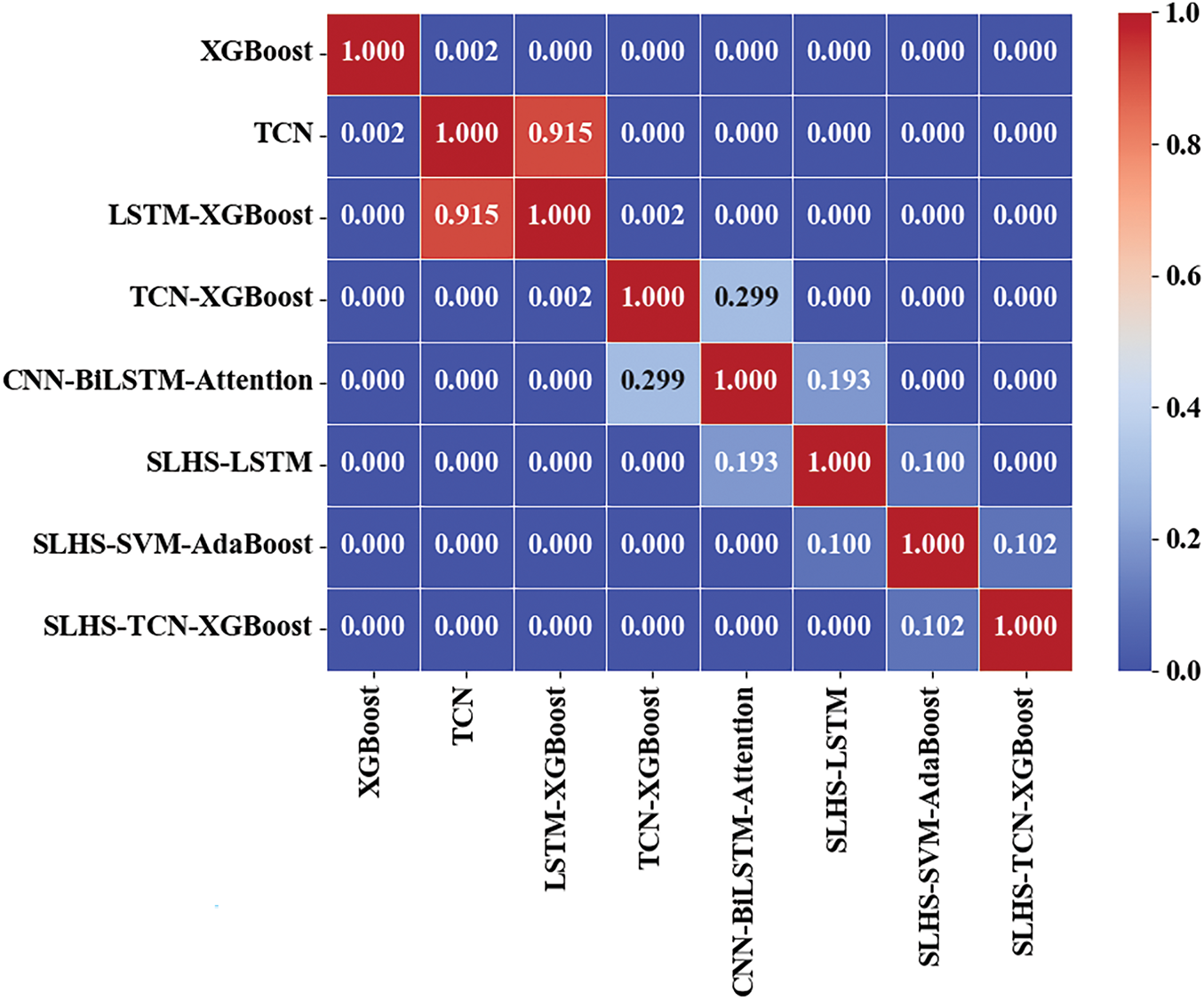
Figure 9: Correlation heat map of MAPE variability of different prediction models
The correlation between LSTM-XGBoost and TCN-XGBoost is high, reaching 0.915, indicating that the prediction results of the two models have strong similarity. Other combination models, such as CNN-BiLSTM-Attention, SLHS-LSTM, and SLHS-SVM-AdaBoost, also show different degrees of correlation, especially the correlation coefficient between SLHS-SVM-AdaBoost and XGBoost is 0.102, indicating that there is a weak positive correlation between the two. Overall, the correlation coefficients between most models are low, which shows that the prediction characteristics of the models are quite different and they are highly independent of each other, emphasizing the diversity and complementarity of model selection.
In order to verify the stability and reliability of different models under different conditions, we conducted the following robustness tests: cross-validation and noise test. These tests are designed to evaluate the performance of the model under changes in data distribution and noise interference.
Cross-validation is a standard method for evaluating the generalization ability of a model. We use 5-fold cross-validation to randomly divide the dataset into 5 subsets, use 4 of them for training in turn, and use the remaining 1 subset for testing, repeat 5 times, and calculate the average performance index. As shown in Fig. 10, the RMSE distribution of different models in 5-fold cross-validation, the box plot shows the error distribution range and median of each model, the RMSE distribution of the SLHS-TCN-XGBoost model is more concentrated, and the overall fluctuation is small, indicating that the model shows high stability on different data subsets.

Figure 10: RMSE distribution of different models in 5-fold cross validation
The median of RMSE is around 500, and the box is relatively compact, indicating that the error distribution of the model is relatively uniform and the deviation is small. In addition, there are no significant outliers or extreme outliers in the upper and lower limits of the box plot, which further verifies the robustness and consistency of SLHS-TCN-XGBoost in different folds. By comparing with other models, it can be seen that SLHS-TCN-XGBoost performs better than many other models in cross validation, especially in terms of lower RMSE values and stronger stability, highlighting its advantages in generalization ability. Overall, the performance of the model is highly reliable and can maintain consistent prediction accuracy under different data partitions, further verifying its effectiveness as a robust model.
To comprehensively evaluate the robustness of the model under different noise conditions, we added three types of noise to the test data: Gaussian noise, spike noise, and seasonal anomalies, and recalculated the RMSE value of each model. The specific noise addition method and analysis process are as follows:
Gaussian noise is a common way to simulate random errors or sensor noise. 5% Gaussian noise was added to the test data, and the performance of the model was re-evaluated. Gaussian noise was added to the true value
where
Spike noise is a type of noise that simulates extreme values or outliers. To generate spike noise, we randomly select 5% of the samples (a total of 132 samples) in the test data and multiply the values of these samples by a random amplification factor (ranging from 10 to 20 times). The equation is as follows:
Among them,
Seasonal outliers simulate periodic fluctuations or seasonal disturbances. In the test set data, we added sinusoidal fluctuations in a specific time period to simulate seasonal changes. The generated perturbation equation is:
Among them,

Figure 11: RMSE results of the model under different noises
Under different noise conditions, the RMSE values of all models increased. For Gaussian noise, the RMSE of the XGBoost model increased from 1197.59 to 1210.34, an increase of about 1.07%, indicating that its robustness to random noise is poor. The RMSE of deep learning models such as TCN, LSTM-XGBoost, TCN-XGBoost, and CNN-BiLSTM-Attention also increased, among which the RMSE of CNN-BiLSTM-Attention under Gaussian noise increased by about 2.7%, showing a certain degree of stability. In contrast, the growth of fusion methods such as SLHS-LSTM, SLHS-SVM-AdaBoost, and SLHS-TCN-XGBoost is smaller, especially SLHS-TCN-XGBoost, whose RMSE only increased from 147.64 to 168.79, an increase of about 14.3%, still maintaining the lowest absolute error level among all models, reflecting a strong anti-noise ability.
Under the interference of Spike noise, the RMSE of each model generally increased more significantly. The RMSE of the XGBoost model soared to 1305, TCN and LSTM-XGBoost increased to 980 and 945, respectively, and the CNN-BiLSTM-Attention model also increased to 658, indicating that such sudden extreme outliers have a great impact on both traditional machine learning and deep learning models. However, the RMSE of the SLHS-TCN-XGBoost model under Spike noise only increased to 176, an increase of about 19.2%, which is much lower than other models, further proving the advantage of this method in dealing with extreme noise disturbances.
Under the seasonal anomaly, the RMSE of each model showed a moderate upward trend as a whole. The RMSE of XGBoost, TCN, LSTM-XGBoost, TCN-XGBoost, and CNN-BiLSTM-Attention increased to 1240, 975, 930, 690, and 635, respectively, and the increase was within a reasonable range. In contrast, the SLHS series models still show stronger robustness, especially the SLHS-TCN-XGBoost model, whose RMSE only increased to 170.5, with a smaller fluctuation than other comparison models.
In summary, SLHS-TCN-XGBoost shows extremely high stability and robustness under various noise conditions. Not only does it have the smallest absolute error, but also its performance degradation is significantly lower than other single models or simple integrated models when facing Gaussian noise, pulse anomalies, and seasonal interference, which fully verifies the superiority of the proposed method in complex interference environments.
In order to deeply analyze the prediction error of the model, we conducted error distribution analysis and error source analysis. These analyses aim to reveal the prediction accuracy of the model and the main sources of error, and provide direction for subsequent model optimization.
5.3.1 Error Distribution Analysis
Error distribution analysis is an important method to evaluate the prediction accuracy of the model. We calculated the prediction error (Error) of each model, defined as:
Among them, Predicted is the predicted value of the model, and Actual is the actual value. The comparison of the error distribution of different models in the prediction process is shown in Fig. 12. The error distribution of each model has obvious differences.

Figure 12: Comparison of error distribution of different prediction models
The error distribution of the XGBoost model is relatively concentrated, showing a sharp peak, mainly concentrated between 0% and 10%, indicating that most of its prediction errors are small, but there are also certain deviations. In contrast, the error distribution of the SLHS-TCN-XGBoost model is relatively smoother, and the peak offset is closer to 0%, indicating that it has higher accuracy and consistency in the prediction process. Most of the errors of SLHS-TCN-XGBoost are concentrated between −5% and 5%, and there are almost no significant extreme errors, which verifies its robustness in complex tasks.
From the perspective of the error distribution, the error of SLHS-TCN-XGBoost is closer to zero than other models, showing higher prediction accuracy and less systematic deviation. In contrast, although models such as LSTM-XGBoost and TCN-XGBoost also have smaller errors, their error distribution shows a wider range and a longer tail, indicating that larger errors may occur in some cases. Overall, the error distribution of all models shows certain normality characteristics, but SLHS-TCN-XGBoost shows higher centralization in mean and standard deviation, which is significantly better than other models.
The error curves shown in the figure are all centered on 0%, and the red dotted line marks the position of zero error. The error distribution curve of SLHS-TCN-XGBoost has the highest frequency close to the zero-error position, further verifying that it is the most accurate among all models. These results show that SLHS-TCN-XGBoost can provide accurate prediction results in most cases, with small errors and stable distribution, highlighting its advantages in practical applications.
In order to further analyze the source of the model’s prediction error, we grouped the errors according to season and time, aiming to identify the impact of different factors on the model’s prediction accuracy. After grouping by season and time, we calculated the average error of each group to reveal the performance fluctuations of the model in each time period. When grouping by season, we divided the data by quarter (Q1: January–March, Q2: April–June, Q3: July–September, Q4: October–December) and calculated the average error for each quarter. The specific calculation equation is as follows:
where

Figure 13: Seasonal and temporal error analysis of different models
From the results of seasonal error analysis, the SLHS-TCN-XGBoost model performed the most stably in all quarters, and its error fluctuated less between quarters, especially in Q3 (July–September) and Q4 (October–December), where it showed obvious advantages and the average error was close to zero, indicating that the model had the strongest adaptability to seasonal changes. In contrast, the XGBoost and TCN models had larger errors in Q1 (January–March) and Q2 (April–June), especially XGBoost, whose error in Q2 reached nearly 4%, indicating that its performance was poor in some seasons.
In terms of temporal error analysis, the SLHS-TCN-XGBoost model had smaller error fluctuations within 24 h of the day, and compared with other models, its error remained at a lower level in most periods, especially in the early morning and evening (0–5 h), where it performed particularly stably. The error of the XGBoost model fluctuated significantly in multiple time periods, especially between 10 and 14 o’clock, with an error value higher than 10%. This indicates that XGBoost is susceptible to noise or data fluctuations in certain time periods, resulting in large errors.
Overall, the SLHS-TCN-XGBoost model performs most stably and accurately in seasonal and temporal error analysis, especially in Q3 and Q4 and throughout the day, where the error remains within a low range, verifying its superiority and robustness in processing complex time series data.
In machine learning models, the choice of hyperparameters has an important impact on model performance. To gain a deeper understanding of the performance of the SLHS-TCN-XGBoost model in power load forecasting, we conducted a hyperparameter sensitivity analysis. This section will analyze the sensitivity of the model to several key hyperparameters, including the learning rate and tree depth of XGBoost, the convolution kernel size of TCN, and the feature selection regularization parameter of SLHS. The hyperparameter settings in this study refer to Section 4.2. By adjusting and evaluating these hyperparameters, we aim to determine the optimal hyperparameter combination and further improve the prediction accuracy and generalization ability of the model.
We conducted a sensitivity analysis on the learning rate of XGBoost. The learning rate controls the pace of each update and affects the convergence speed and stability of the model. A smaller learning rate can usually improve the stability of the model, but the training time is longer; while a larger learning rate may accelerate convergence, it is also easy to cause overfitting or instability of the model. Based on this, we selected learning rates of 0.01, 0.05, 0.1, and 0.2 for experiments to test their effects on the RMSE and MAPE of the model. The maximum depth of the XGBoost tree also affects the model’s fitting ability and computational efficiency. A larger tree depth can increase the model’s expressiveness, but may lead to overfitting. Therefore, we selected tree depths of 6, 8, 10, and 12 for testing.
In addition, the size of the convolution kernel in the TCN model has an important impact on the feature extraction effect. The size of the convolution kernel directly determines the model’s ability to perceive local features of time series data. Larger convolution kernels can capture dependencies over longer time spans but may reduce the model’s ability to process fine-grained time series features. In this experiment, we selected convolution kernel sizes of 3, 5, 7, and 9 for sensitivity testing.
Finally, the regularization parameter λ in the SLHS model controls the strength of feature selection. Too small a λ value may lead to overfitting, while too large a λ value may oversimplify the model and lead to the loss of important features. To analyze the impact of the λ value, we selected λ as 0.01, 0.1, 1.0, and 10.0 for experiments to evaluate its impact on the prediction accuracy of the model.
5.4.1 Sensitivity Analysis of XGBoost Hyperparameters
We first conducted a sensitivity analysis on the learning rate and tree depth of the XGBoost model. According to the combination of different learning rates and tree depths, the RMSE and MAPE values of the model are listed in Table 10.
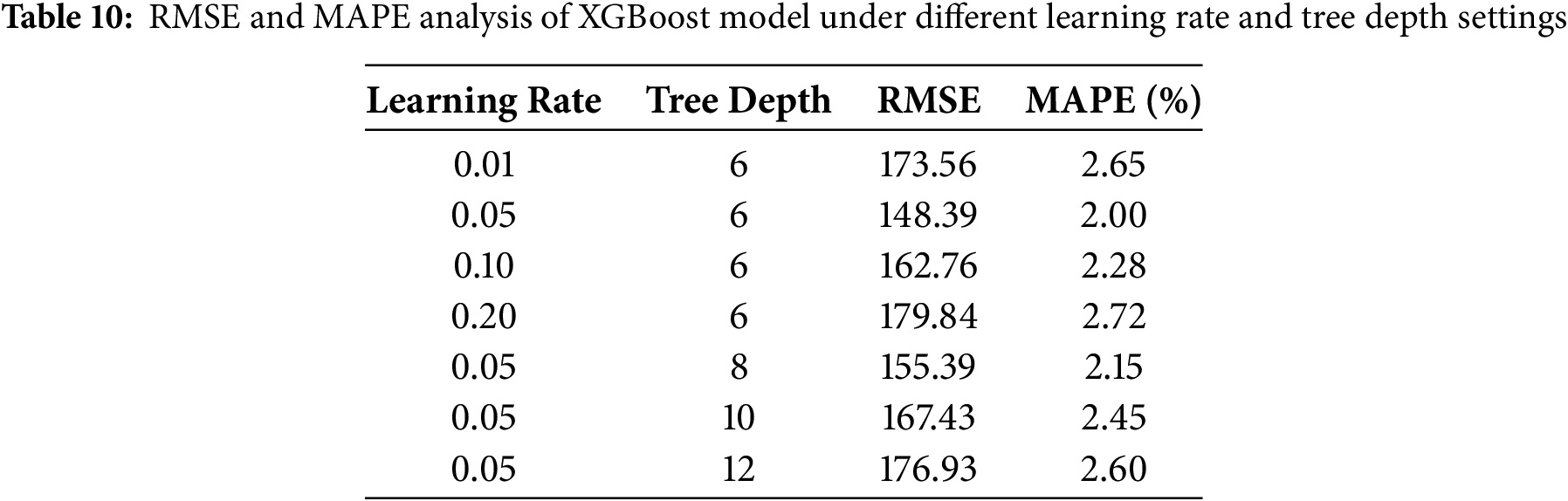
It can be seen from Table 10 that with the increase of learning rate, the RMSE and MAPE values increase, especially when the learning rate is 0.2, the prediction error of the model increases significantly, indicating that too high a learning rate may lead to unstable model performance. At the same time, the influence of tree depth on model performance is more obvious. With the increase of tree depth, RMSE and MAPE gradually increase, especially when the depth is 12, showing a large overfitting trend.
5.4.2 Sensitivity Analysis of TCN Convolution Kernel Size
Next, we conduct a sensitivity analysis on the convolution kernel size of the TCN model. To examine the impact of different convolution kernel sizes on the prediction performance of the model, we used convolution kernel sizes of 3, 5, 7, and 9 for experiments, and the results are shown in Table 11.

Table 11 shows that when the convolution kernel size is 3, the RMSE and MAPE values of the model are the lowest, indicating that smaller convolution kernels can better capture the local features of time series data. As the size of the convolution kernel increases, the error of the model gradually increases, which may be because the larger convolution kernel captures too broad features, resulting in loss of information. Therefore, in practical applications, choosing an appropriate convolution kernel size is crucial to improving the prediction accuracy of the TCN model.
5.4.3 Sensitivity Analysis of SLHS Regularization Parameter λ
In the SLHS model, the regularization parameter

As can be seen from Table 12, a smaller
Through the hyperparameter sensitivity analysis of the XGBoost, TCN, and SLHS models, we found that appropriate hyperparameter settings can significantly improve the prediction accuracy of the model. In XGBoost, the combination of a smaller learning rate and a tree depth of 6 can effectively avoid overfitting, while the TCN model with a convolution kernel size of 3 performs best. For SLHS, a smaller regularization parameter
6.1 Comparative Performance Analysis
The SLHS-TCN-XGBoost model shows superior performance compared to the baseline model and the state-of-the-art model, with an MAE of 112.08, an RMSE of 148.39, and an MAPE of 2%, which are 87.37%, 87.35%, and 87.43% lower than the XGBoost model alone (Table 3). This significant improvement highlights the effectiveness of SLHS dimensionality reduction, TCN temporal feature extraction, and XGBoost ensemble learning.
Comparison with Traditional Models: The model outperformed traditional methods and simpler machine learning models, which struggle with high-dimensional, nonlinear data (Section 2). For instance, the SLHS-TCN-XGBoost’s MAPE was 6–8 times lower than that of CNN-BiLSTM-Attention (7.94%) and TCN-XGBoost (9.95%) (Table 3), highlighting its ability to capture complex temporal dependencies.
Comparison with Hybrid Models: While SLHS-SVM-AdaBoost (MAPE 3.98%) and SLHS-LSTM (5.99%) showed competitive results, the proposed model’s fusion strategy (weighted ensemble of SLHS, TCN, and XGBoost) reduced errors by 50%–60% further (Table 7). This aligns with findings in Section 3.4, where the weighted fusion (Eq. (5)) optimally combined model strengths.
Statistical tests confirmed these differences: the t-test (Table 8) and Tukey HSD post hoc test (Table 9) revealed that SLHS-TCN-XGBoost’s improvements were significant (p < 0.05) across all comparisons, with the largest MAPE reduction (98.17%) on critical days (Table 7).
6.2 Robustness and Generalizability
The model exhibited strong robustness under noise and data variability:
Noise Resilience: When subjected to 5% Gaussian noise, the SLHS-TCN-XGBoost model exhibited a controlled RMSE increase from 147.64 to 168.79, representing a rise of approximately 14.3%, which remains significantly lower than that observed in other models. In contrast, the RMSE of the XGBoost model increased from 1197.59 to 1210.34 under the same noise conditions, reflecting a less stable response to random perturbations (Fig. 11). This superior noise resilience of the SLHS-TCN-XGBoost model can be attributed to the feature smoothing capability of the SLHS component and the robustness of TCN’s dilated convolutions, which effectively attenuate noise while preserving key temporal structures in the data (Section 5.2.2).
Cross-Validation: In 5-fold cross-validation, the model’s RMSE distribution was tightly clustered (Fig. 10), indicating consistent performance across data subsets. Seasonal error analysis further validated its reliability, with MAPE ≤ 1% in Q3/Q4 and nighttime hours (Fig. 13).
Generalizability across Regions: While the current evaluation is based on the Seoul metropolitan area in South Korea, the model is designed with modular components (SLHS for feature filtering, TCN for temporal modeling, and XGBoost for ensemble prediction), allowing it to adapt to other datasets with different climatic conditions, regional load behaviors, and grid structures. Future work will apply the model to datasets from regions with diverse characteristics, such as tropical or arid climates, or more decentralized energy grids, to validate its transferability and explore any necessary regional adjustments in model parameters.
6.3 Interpretation of Performance Differences
The SLHS-TCN-XGBoost’s advantages stem from three key factors:
Feature Selection: SLHS’s latent heatmap smoothing (Eq. (1)) eliminated redundant features, reducing overfitting. Sensitivity analysis (Table 12) confirmed that λ = 0.01 optimally balanced sparsity and feature retention.
Temporal Modeling: TCN’s dilated causal convolutions (Eq. (2)) captured long-term dependencies more effectively than LSTM-based models (Section 3.2). The sensitivity of TCN’s kernel size (Table 11) revealed that smaller kernels (size 3) better localized temporal patterns.
Ensemble Learning: XGBoost’s regularization (Eq. (4)) mitigated overfitting, while its sensitivity to learning rate (Table 10) underscored the importance of fine-tuning (optimal rate: 0.05).
6.4 Limitations and Future Directions
Computational Cost: While the model achieved high accuracy, its training time exceeded simpler models (Section 4.2). Future work could optimize SLHS’s dimensionality reduction or explore lightweight TCN architectures.
Interpretability: the model’s “black box” nature limits insights into feature contributions. Techniques like SHapley Additive exPlanations analysis could enhance explainability for grid operators.
Geographical Generalizability: the current validation is limited to the Seoul metropolitan area, which may not represent the full diversity of power demand patterns across different regions. While the model demonstrates strong performance on this dataset, its effectiveness may vary when applied to regions with different climate conditions, varied industrial structures, distinct seasonal patterns, and alternative energy mix compositions. Future work should systematically evaluate the model’s performance across multiple geographical regions to establish its broader applicability.
External Factors: the model currently relies primarily on historical load and weather data, which are the most readily available and influential features for short- to medium-term forecasting. However, external factors such as economic activities, policy changes, and unexpected events can also significantly impact electricity demand. Future work could explore integrating macroeconomic indicators and event-driven features to further improve the robustness and adaptability of the model across diverse real-world scenarios.
Static Dimensionality Reduction: in the current framework, SLHS is applied statically for feature selection and dimensionality reduction based on the overall dataset distribution. While this approach effectively reduces feature redundancy and computational burden, it does not adapt dynamically to potential temporal shifts in data characteristics. Future work could investigate dynamic feature selection strategies that continuously adjust to evolving data patterns to further enhance model flexibility and real-time prediction accuracy.
Temporal Information Loss during Feature Selection: the current SLHS-based feature selection and dimensionality reduction process operates without explicitly considering temporal dependencies. While this approach effectively reduces dimensionality and computational complexity, it may inadvertently discard time-sensitive features, potentially impacting the model’s ability to capture long-term trends and seasonal variations in load demand. Future work could explore time-aware feature selection techniques, such as dynamic SLHS with sliding windows, sequential feature selection, or attention-based feature importance adjustment, to better preserve critical temporal information.
Implicit Treatment of Causality: while the model demonstrates strong predictive performance, it currently treats causality implicitly rather than explicitly. The correlation-based approach may be susceptible to confounding, particularly in scenarios where novel policy interventions change underlying demand patterns, structural breaks occur in the energy market, or previously unobserved variables become significant drivers. Future work should incorporate more formal causal modeling approaches, such as structural causal models or Granger causality frameworks, to better distinguish true causal relationships from spurious correlations and enhance robustness under evolving market conditions.
The model’s accuracy (MAPE ≤ 2%) and noise resilience make it suitable for real-world grid management, particularly in scenarios requiring high-frequency forecasts. Seasonal stability (Q3/Q4 errors < 1%) also supports its use in long-term capacity planning.
The superior performance of the SLHS-TCN-XGBoost model (MAPE = 2%) compared to traditional methods (XGBoost’s MAPE = 15.91%) has significant real-world implications for power system operators. For a utility serving 10 million customers, a 2% improvement in MAPE can reduce dispatch costs by $2 million to $3.5 million per year, or 0.5% to 0.9% of total operating expenses. In addition to saving money, the model’s higher accuracy reduces key risks such as load shedding (avoiding approximately 4 h of blackouts per year during peak demand) and renewable energy curtailment (reducing wasted wind/solar generation by 12% through better demand coordination). These benefits are particularly important in high-risk environments such as hospitals and data centers, where a reliable power supply is critical. The symmetric error distribution of SLHS-TCN-XGBoost (Fig. 12) further ensures balanced risk management, avoiding costly power shortages and inefficient overgeneration.
Combining these findings with industry benchmark data from the Korea Power Exchange (KPX) and the International Energy Agency (IEA), it is confirmed that even a slight improvement in forecast accuracy can bring measurable economic benefits, especially in markets with high renewable energy penetration. Therefore, the SLHS-TCN-XGBoost framework not only advances predictive modeling, but also brings tangible value to grid operators, enhancing its practical application value in modern energy systems.
This study presents the SLHS-TCN-XGBoost model, a novel hybrid approach for power demand forecasting that integrates SLHS for dimensionality reduction, TCN for temporal feature extraction, and XGBoost for ensemble learning. Through a large number of experiments on the three-year power load dataset of Seoul, South Korea, the model showed excellent performance, with MAE, RMSE, and MAPE reaching 112.08, 148.39, and 2%, respectively, which were significantly improved by 87.37%, 87.35%, and 87.43% respectively compared with the baseline XGBoost model. The model’s robustness is further validated through cross-validation, noise perturbation tests, and statistical significance analyses, confirming its stability and adaptability across different seasonal and temporal conditions.
The research process involved systematic data preprocessing, feature selection, and hyperparameter optimization to ensure the model’s effectiveness. Key findings highlight the model’s ability to capture complex temporal dependencies and nonlinear relationships in power demand data, outperforming traditional and advanced forecasting methods. The SLHS-TCN-XGBoost framework not only enhances prediction accuracy but also exhibits strong resilience to noise and data variability, making it a reliable solution for real-world power system applications.
The implications of this study extend beyond improved forecasting accuracy. By integrating SLHS, TCN, and XGBoost, the model provides a scalable and efficient framework for handling high-dimensional and noisy time-series data, offering valuable insights for energy management and grid optimization. The methodological advancements presented here could inspire further innovations in hybrid modeling for other time-series forecasting tasks, such as renewable energy generation prediction or smart grid load balancing.
Despite its strengths, the study acknowledges certain limitations. The model’s performance is constrained by the quality and scope of the input data, and its computational complexity may pose challenges for real-time applications with extremely large datasets. Future research could focus on enhancing the model’s interpretability, reducing computational overhead, and extending its applicability to multi-step forecasting and other energy-related prediction tasks.
Building on these findings, future research can be carried out from the following aspects: Explore more efficient data preprocessing and feature selection methods to further improve the prediction accuracy and robustness of the model. Multi-scale analysis of power demand data can be combined with technologies such as wavelet transform or Empirical mode decomposition (EMD) to capture the load variation law at different time scales. Second, deep learning algorithms can be combined to further optimize the time series modeling ability of the model, especially in capturing complex nonlinear relationships in power demand. The Transformer model can capture global dependencies in time series through the self-attention mechanism, while GNNs can be used to model spatial dependencies in power systems. In addition, the interpretability of the model can be studied, and the decision-making process of the model can be revealed through visualization technology and feature importance analysis, providing more intuitive support for the planning and operation of the power system. The contribution of each feature in the SLHS-TCN-XGBoost model to the prediction results can be analyzed through the SHAP value, thereby identifying the key factors affecting power demand. Finally, the model is applied to more practical scenarios to verify its adaptability and versatility in different environments. The application potential of the SLHS-TCN-XGBoost model in renewable energy generation forecasting and power market bidding can be studied. Through continuous optimization and innovation, the SLHS-TCN-XGBoost model is expected to play a greater role in the field of power demand forecasting and provide strong support for the intelligent development of the power industry.
Acknowledgement: The authors thank the Mahasarakham University and Korea Electric Power Corporation (KEPCO) Open Data Portal for supporting this work.
Funding Statement: This research was financially supported by Mahasarakham University for Piyapatr Busababodhin’s work. Guoqing Chen’s research was supported by Chengdu Jincheng College Green Data Integration Intelligence Research and Innovation Project (No. 2025–2027) and the High-Quality Development Research Center Project in the Tuojiang River Basin (No. TJGZL2024-07). Additionally, the project received funding from the Open Fund of Wuhan Gravitation and Solid Earth Tides, National Observation and Research Station (No. WHYWZ202406), as well as the Scientific Research Fund of the Institute of Seismology, CEA, and the National Institute of Natural Hazards, MEM (No. IS202236328).
Author Contributions: Conceptualization, Tianwen Zhao; methodology, Tianwen Zhao; software, Tianwen Zhao; validation, Guoqing Chen and Cong Pang; formal analysis, Piyapatr Busababodhin, Tianwen Zhao and Guoqing Chen; investigation, Tianwen Zhao; resources, Tianwen Zhao; data curator, Tianwen Zhao; writing original draft preparation, Tianwen Zhao; writing review and editing, Guoqing Chen and Piyapatr Busababodhin; visualization, Cong Pang and Tianwen Zhao; supervision, Piyapatr Busababodhin; project administration, Piyapatr Busababodhin, Cong Pang and Guoqing Chen. All authors reviewed the results and approved the final version of the manuscript.
Availability of Data and Materials: Data available on request from the authors. The data that support the findings of this study are available from the Corresponding Author, Piyapatr Busababodhin, upon reasonable request.
Ethics Approval: Not applicable.
Conflicts of Interest: The authors declare no conflicts of interest to report regarding the present study.
Abbreviations
| SLHS | Sequential Latin hypercube sampling |
| TCN | Temporal Convolutional Network |
| XGBoost | eXtreme Gradient Boosting |
| SVM | Support vector machines |
| LSTM | Long short-term memory network |
| CNN | Convolutional neural network |
| RNN | Recurrent neural network |
| BiLSTM | Bidirectional Long Short-Term Memory |
| GNNs | Graph neural networks |
| TPA | Temporal pattern attention |
| CSSA | Chaos sparrow search algorithms |
| MSE | Mean square error |
| RMSE | Root mean square error |
| MAE | Mean absolute error |
| R2 | Coefficient of determination |
| MAPE | Mean absolute percentage error |
| EMD | Empirical mode decomposition |
References
1. Liu W, Mao Z. Short-term photovoltaic power forecasting with feature extraction and attention mechanisms. Renew Energy. 2024;226(22):120437. doi:10.1016/j.renene.2024.120437. [Google Scholar] [CrossRef]
2. Zhang L, Jánošík D. Enhanced short-term load forecasting with hybrid machine learning models: CatBoost and XGBoost approaches. Expert Syst Appl. 2024;241(4):122686. doi:10.1016/j.eswa.2023.122686. [Google Scholar] [CrossRef]
3. Zhou D, Liu Y, Wang X, Wang F, Jia Y. Combined ultra-short-term photovoltaic power prediction based on CEEMDAN decomposition and RIME optimized AM-TCN-BiLSTM. Energy. 2025;134847. doi:10.1016/j.energy.2025.134847. [Google Scholar] [CrossRef]
4. Harikrishnan GR, Sreedharan S. Advanced short-term load forecasting for residential demand response: an XGBoost-ANN ensemble approach. Electr Power Syst Res. 2025;242(13):111476. doi:10.1016/j.epsr.2025.111476. [Google Scholar] [CrossRef]
5. Pang S, Zou L, Zhang L, Wang H, Wang Y, Liu X, et al. A hybrid TCN-BiLSTM short-term load forecasting model for ship electric propulsion systems combined with multi-step feature processing. Ocean Eng. 2025;316:119808. doi:10.1016/j.oceaneng.2024.119808. [Google Scholar] [CrossRef]
6. Gong J, Qu Z, Zhu Z, Xu H, Yang Q. Ensemble models of TCN-LSTM-LightGBM based on ensemble learning methods for short-term electrical load forecasting. Energy. 2025;134757. doi:10.1016/j.energy.2025.134757. [Google Scholar] [CrossRef]
7. Fan GF, Han YY, Li JW, Peng LL, Yeh YH, Hong WC. A hybrid model for deep learning short-term power load forecasting based on feature extraction statistics techniques. Expert Syst Appl. 2024;238:122012. doi:10.1016/j.eswa.2023.122012. [Google Scholar] [CrossRef]
8. Hyndman RJ, Athanasopoulos G. Forecasting: principles and practice. 2nd ed. Melbourne, Australia: OTexts; 2018. [Google Scholar]
9. Smola AJ, Schölkopf B. A tutorial on support vector regression. Stat Comput. 2004;14(3):199–222. doi:10.1023/B:STCO.0000035301.49549.88. [Google Scholar] [CrossRef]
10. Breiman L. Random forests. Mach Learn. 2001;45(1):5–32. doi:10.1023/A:1010933404324. [Google Scholar] [CrossRef]
11. Hochreiter S, Schmidhuber J. Long short-term memory. Neural Comput. 1997;9(8):1735–80. doi:10.1162/neco.1997.9.8.1735. [Google Scholar] [PubMed] [CrossRef]
12. LeCun Y, Bengio Y, Hinton G. Deep learning. Nature. 2015;521(7553):436–44. doi:10.1038/nature14539. [Google Scholar] [PubMed] [CrossRef]
13. Zhang G, Eddy Patuwo B, Hu MY. Forecasting with artificial neural networks: the state of the art. Int J Forecast. 1998;14(1):35–62. doi:10.1016/S0169-2070(97)00044-7. [Google Scholar] [CrossRef]
14. Bai S, Kolter JZ, Koltun V. An empirical evaluation of generic convolutional and recurrent networks for sequence modeling. arXiv:1803.01271. 2018. [Google Scholar]
15. Chen T, Guestrin C. XGBoost: a scalable tree boosting system. In: Proceedings of the 22nd ACM SIGKDD International Conference on Knowledge Discovery and Data Mining; 2016 Aug 13–17; San Francisco, CA, USA. New York, NY, USA: ACM; 2016. p. 785–94. doi:10.1145/2939672.2939785. [Google Scholar] [CrossRef]
16. Abbasimehr H, Paki R, Bahrini A. A novel XGBoost-based featurization approach to forecast renewable energy consumption with deep learning models. Sustain Comput Inform Syst. 2023;38(2):100863. doi:10.1016/j.suscom.2023.100863. [Google Scholar] [CrossRef]
17. Fan C, Nie S, Xiao L, Yi L, Wu Y, Li G. A multi-stage ensemble model for power load forecasting based on decomposition, error factors, and multi-objective optimization algorithm. Int J Electr Power Energy Syst. 2024;155:109620. doi:10.1016/j.ijepes.2023.109620. [Google Scholar] [CrossRef]
18. Fan C, Nie S, Xiao L, Yi L, Li G. Short-term industrial load forecasting based on error correction and hybrid ensemble learning. Energy Build. 2024;313(4):114261. doi:10.1016/j.enbuild.2024.114261. [Google Scholar] [CrossRef]
19. Zeng S, Xiang XJ, Dou YP, Du JC, He G. UAV data link anti-interference via SLHS-SVM-AdaBoost algorithm: classification prediction and route planning. J Electron Sci Technol. 2024;22(4):100279. doi:10.1016/j.jnlest.2024.100279. [Google Scholar] [CrossRef]
20. Fan S, Hyndman RJ. Short-term load forecasting based on a semi-parametric additive model. IEEE Trans Power Syst. 2012;27(1):134–41. doi:10.1109/TPWRS.2011.2162082. [Google Scholar] [CrossRef]
21. Wen J, Wang Z. Short-term power load forecasting with hybrid TPA-BiLSTM prediction model based on CSSA. Comput Model Eng Sci. 2023;136(1):749–65. doi:10.32604/cmes.2023.023865. [Google Scholar] [CrossRef]
22. Wang J, Li J, Wang X, Wang T, Sun Q. A quality prediction model based on CNN-BiNLSTM-attention. Environ Dev Sustain. 2022;1–16. doi:10.1007/s10668-021-02102-8. [Google Scholar] [CrossRef]
23. Semmelmann L, Henni S, Weinhardt C. Load forecasting for energy communities: a novel LSTM-XGBoost hybrid model based on smart meter data. Energy Inform. 2022;5(Suppl 1):24. doi:10.1186/s42162-022-00212-9. [Google Scholar] [CrossRef]
24. Li R, Jiang P, Yang H, Li C. A novel hybrid forecasting scheme for electricity demand time series. Sustain Cities Soc. 2020;55(2):102036. doi:10.1016/j.scs.2020.102036. [Google Scholar] [CrossRef]
25. Zhang J, Wei YM, Li D, Tan Z, Zhou J. Short term electricity load forecasting using a hybrid model. Energy. 2018;158(1):774–81. doi:10.1016/j.energy.2018.06.012. [Google Scholar] [CrossRef]
26. Zhang J, Siya W, Zhongfu T, Anli S. An improved hybrid model for short term power load prediction. Energy. 2023;268(27):126561. doi:10.1016/j.energy.2022.126561. [Google Scholar] [CrossRef]
27. Tian C, Liu Y, Zhang G, Yang Y, Yan Y, Li C. Transfer learning based hybrid model for power demand prediction of large-scale electric vehicles. Energy. 2024;300(14):131461. doi:10.1016/j.energy.2024.131461. [Google Scholar] [CrossRef]
28. Yang Q, Zhang J, Zhang J, Sun C, Xie S, Liu S, et al. Graph transformer network incorporating sparse representation for multivariate time series anomaly detection. Electronics. 2024;13(11):2032. doi:10.3390/electronics13112032. [Google Scholar] [CrossRef]
29. Lotfipoor A, Patidar S, Jenkins DP. Deep neural network with empirical mode decomposition and Bayesian optimisation for residential load forecasting. Expert Syst Appl. 2024;237(1):121355. doi:10.1016/j.eswa.2023.121355. [Google Scholar] [CrossRef]
30. Ray P, Ganguli B, Chakrabarti A. Multivariate bayesian time-series model with multi-temporal convolution network for forecasting stock market during COVID-19 pandemic. Int J Comput Intell Syst. 2024;17(1):170. doi:10.21203/rs.3.rs-3948985/v1. [Google Scholar] [CrossRef]
31. Qu H, Kuang H, Wang Q, Li J, You L. A physics-informed and attention-based graph learning approach for regional electric vehicle charging demand prediction. IEEE Trans Intell Transp Syst. 2024;25(10):14284–97. doi:10.1109/TITS.2024.3401850. [Google Scholar] [CrossRef]
32. Li X, Wang Z, Yang C, Bozkurt A. An advanced framework for net electricity consumption prediction: incorporating novel machine learning models and optimization algorithms. Energy. 2024;296:131259. doi:10.1016/j.energy.2024.131259. [Google Scholar] [CrossRef]
33. Dai Y, Yu W, Leng M. A hybrid ensemble optimized BiGRU method for short-term photovoltaic generation forecasting. Energy. 2024;299(7):131458. doi:10.1016/j.energy.2024.131458. [Google Scholar] [CrossRef]
34. Jadon A, Patil A, Jadon S. A comprehensive survey of regression-based loss functions for time series forecasting. In: International Conference on Data Management, Analytics & Innovation. Singapore: Springer Nature Singapore; 2024. p. 117–47. doi:10.1007/978-981-97-3245-6_9. [Google Scholar] [CrossRef]
35. Shen C, Wu J. Research on credit risk of listed companies: a hybrid model based on TCN and DilateFormer. Sci Rep. 2025;15(1):2599. doi:10.1038/s41598-025-86371-7. [Google Scholar] [PubMed] [CrossRef]
36. Tahir MF, Tzes A, Yousaf MZ. Enhancing PV power forecasting with deep learning and optimizing solar PV project performance with economic viability: a multi-case analysis of 10 MW Masdar project in UAE. Energy Convers Manag. 2024;311:118549. doi:10.1016/j.enconman.2024.118549. [Google Scholar] [CrossRef]
37. Hanifi S, Cammarono A, Zare-Behtash H. Advanced hyperparameter optimization of deep learning models for wind power prediction. Renew Energy. 2024;221(15):119700. doi:10.1016/j.renene.2023.119700. [Google Scholar] [CrossRef]
38. Zhao Y, Zhang W, Liu X. Grid search with a weighted error function: hyper-parameter optimization for financial time series forecasting. Appl Soft Comput. 2024;154(1):111362. doi:10.1016/j.asoc.2024.111362. [Google Scholar] [CrossRef]
39. Deng S, Inekwe J, Smirnov V, Wait A, Wang C. Seasonality in deep learning forecasts of electricity imbalance prices. Energy Econ. 2024;137(8):107770. doi:10.1016/j.eneco.2024.107770. [Google Scholar] [CrossRef]
40. Hu X, Li H, Si C. Improved composite model using metaheuristic optimization algorithm for short-term power load forecasting. Electr Power Syst Res. 2024;241(4):111330. doi:10.1016/j.epsr.2024.111330. [Google Scholar] [CrossRef]
41. Gong J, Qu Z, Zhu Z, Xu H. Parallel TimesNet-BiLSTM model for ultra-short-term photovoltaic power forecasting using STL decomposition and auto-tuning. Energy. 2025;320:135286. doi:10.1016/j.energy.2025.135286. [Google Scholar] [CrossRef]
Cite This Article
 Copyright © 2025 The Author(s). Published by Tech Science Press.
This work is licensed under a Creative Commons Attribution 4.0 International License , which permits unrestricted use, distribution, and reproduction in any medium, provided the original work is properly cited.
 Downloads
 Citation Tools