Smooth Boundary Topology Optimization—A New Framework for Movable Morphable Smooth Boundary Method

1  Introduction

Due to the rapid development of additive manufacturing technology, its integration with topology optimization is becoming increasingly close, expanding the design space available for topology optimization. Combining them will be a new revolution with significant development prospects in the modern manufacturing industry [1,2]. However, the final structure produced through topology optimization is generally challenging to be directly used for manufacturing because most of the structural design domains in topology optimization use quadrilateral elements or hexahedral elements, and they inevitably result in jagged boundaries and gray-scale elements. Although many researchers have studied the jagged boundary problem, most solutions involve post-processing after the optimization iterations terminate. Although this method can make the boundaries smoother, it can compromise the advantages of topology optimization, potentially reducing the mechanical properties of the structure and diminishing its engineering value. Therefore, developing an optimization method that achieves smooth boundaries automatically during the optimization process is of great significance.

In 2012, Fu [3] obtained satisfactory optimization results based on the level set optimization method using a geometric reconstruction technique to fit the topology-optimized boundaries. In 2022, Zhang et al. [4] binarized the results of the topology optimization design to obtain the boundaries without gray elements and then extracted the corner points of the boundaries. Finally, the focus of these corner points was fitted to the curve to achieve a smooth and clear boundary. Although this method results in smooth boundaries, the mechanical properties of the overall structure are altered. In 2022, Li et al. [5] used a pre-constructed look-up table to transform the shapes of the boundary elements obtained in topology optimization and finally generated a topology configuration with smooth boundaries, which improved the jagged boundaries. In 2022, Liu et al. [6] employed a topological design method based on discrete variables that were based on SAIP (sequential approximate integer programming) and CRA (canonical relaxation algorithm), which helped to avoid gray elements and achieve clear 0–1 solution in topology optimization.

In addition to post-processing methods, some researchers have also used mesh adaptive refinement. Adaptive mesh refinement algorithms were first proposed by Maute et al. [7] in 1995, using independent mesh analysis and smoothing algorithms. Using cubic spline or Bezier spline approximation not only reduces the number of design variables and obtains smoothed results but also can be directly combined with traditional shape optimization methods. In 2018, Thomás et al. [8] used the Tyson polygonal division of the mesh to implement the adaptive strategy. They applied four numerical examples to validate the comparison between the Tyson polygonal and the complete refinement and found that the adaptive strategy was able to reduce the computation time and obtain clear material distribution and boundaries.

Since the level set optimization method itself can ameliorate the jagged boundary problem, many researchers have combined the method with topology optimization methods with jagged boundaries to solve the problem. In 2018, Da et al. [9] employed node sensitivity to construct a level set function to implicitly determine a smooth structural topology based on the jagged boundary problem that exists in the bidirectional asymptotic structural optimization method. In 2019, Liu et al. [10] proposed a topology optimization method using floating projection for the jagged boundary problem arising from the Bi-directional Evolutionary Structural Optimization (BESO) method, which first uses floating projection constraints to fit the intermediate density elements more closely to the 0/1 design variables, and then uses the zero contour of the level-set function to depict the boundary to obtain the result of a smooth boundary. In 2024, Muayad and Majid [11] proposed a plastic limit probability-based structural topology optimization method utilizing an extended BESO approach. Compared to traditional design methods, this method demonstrates significant improvements in terms of load-bearing capacity, stress intensity, stiffness, and yield load. Gómez-Silva et al. [12] implemented a novel approach to obtain the optimal volume fraction of the materials forming the structure using the BESO method. In 2020, Fu et al. [13] proposed an algorithm for the optimal design of continuum topology based on element volume fraction, which thoroughly investigated the effects of parameters, mesh sizes, and penalty coefficients in the Heaviside smoothing function on the efficiency of performance computation and topology design, and used the zero level-set function to implicitly extract smooth topological boundaries to effectively improve the jagged boundaries.

The development of machine learning, as well as deep learning, makes topology optimization have a lot of development space. In 2021, Yu [14], based on the method of movable deformation components for the unsmooth boundary problem, employed the convolution operator to establish the connection of the topology description functions of the mutually independent formations and utilized the radius of the convolution to control the effect of the smoothness. The topological description function uses the Kreisselmeier-Steinhauser (KS) function instead of the Max function. In 2022, Huang et al. [15] proposed a problem-independent machine learning-enhanced multiresolution topology optimization method based on the Solid Isotropic Material with Penalization (SIMP) method, which focuses on the shape function for structural finite element analysis and establishes the numerical interpolation between the density of the fine mesh elements within the coarse mesh elements and the corresponding nodes of the coarse mesh elements through machine learning implicit relationship between the shape functions.

The Independent Continuum Mapping (ICM) method used for modeling in this study was initially proposed by Sui and Yang [16] in 1996, which restores the independence of topological design variables by removing their dependence on dimensional optimization variables, such as material parameters or geometrical properties. The ICM method represents the presence or absence of elements in a manner that is independent of their specific physical properties. This method overcomes the difficulty encountered in variable-density approaches and similar methods to a certain extent, where it is challenging to handle multi-loading-condition problems when the objective is to optimize compliance. Topology optimization under stress, displacement, frequency, and vibration constraints for continuum structures has been investigated by Peng and others [17–19]. Long et al. [20–22] proposed a node-independent variable-based approach and a hybrid interpolation modeling method to study the topology optimization of a continuum under harmonic response. In 2022, Yan et al. [23] used the power function as a filtering function and investigated the effect of power exponents with different parameters on the convergence of the optimization results. In 2023, Du et al. [24] used an ICM approach to investigate the topology optimization of continuum structures under the consideration of the breakage-safety topology optimization of randomly broken structures in this case. No researcher has studied the sawtooth boundary problem for the ICM method, which also exists in the same way.

This study explores the jagged boundary problem of the ICM method in topology optimization. It develops a topology optimization model with minimum weight as the goal and displacement as the constraint. A new Movable Morphable Smooth Boundary (MMSB) method is proposed. The method uses a triangular mesh as the basic mesh, which can directly improve the jagged boundary in the optimization process without changing the mechanical properties of the structure.

2  Displacement-Constrained Topology Optimization Model Based on the ICM Method

2.1 Establishment of Optimization Model

The topology optimization model based on the ICM (Independent Continuous and Mapping) method with weight minimization as the objective and displacement as the constraint is established as follows:

{Find t∈ENMake W=∑i=1Nwi→mins.t.uj≤u¯j(j=1,…,J)0≤ti_≤ti≤1(i=1,…,N)(1)

where i and j are the index of design variables and the index of constraints, respectively; N and J are the total number of design variables and the total number of displacement constraints, respectively; t is the vector of topology design variables; ti is the i-th variable; EN is an N-dimensional Euclidean space; W is the weight of the structure; wi is the weight of the i-th element; uj is the j-th displacement constraint; u¯j is the upper limit of the j-th displacement constraint

The initial element topology variable values in the entire design domain in the topology optimization model are all 1. During the iteration process, the element topology variable will change, presenting the values as continuous values in the interval [0, 1], for which it is necessary to introduce a filtering function to achieve the transformation between the discrete topology variable and the continuous topology variable.

The filter functions of element weight and element stiffness in the ICM method are given in the following equations:

wi=fw(ti)wi0,ki=fk(ti)ki0(2)

where wi0 and ki0 are the intrinsic weight and stiffness of the i-th element, respectively; ki is the element stiffness of the i-th element; fw is the filter function for element weight; fk is the filter function for element stiffness.

The rational fractional function is chosen to solve the problem, and this filter function can reduce the intermediate gray elements and also improve computational efficiency.

fw(ti)=ti1+qw(1−ti),fk(ti)=ti1+qk(1−ti)(3)

where qw is the parameter of the element weight filter function; qk is the parameter of the element stiffness filter function; qw = 3 and qk = 63 are used in this study [25].

The optimization model built by introducing the filtering function becomes:

{Find t∈ENMake W=∑i=1Nfw(ti)wi0→mins.t.uj(fk(ti))≤u¯j(j=1,…,J)0≤ti_≤ti≤1(i=1,…,N)(4)

2.2 Explicitation of Displacement Constraint

Based on Mohr’s principle, the generalized displacement of any node in the given direction of the structure can be seen as follows:

uj=∑i=1N∫(σiV)TεiJdv(5)

where σiV is the stress vector of the element i by applying one element of imaginary load in the uj displacement direction; εiJ is the strain vector of the element i by applying real load.

Based on the principle of virtual work mentioned in “the work done by the external force on the virtual displacement is equal to the virtual work done by the internal force on the virtual deformation caused by the virtual displacement”, it can be obtained as follows:

∑i=1N∫(σiV)TεiJdv=∑i=1N(uiV)TFiJ(6)

where uiV is the imaginary displacement; FiJ is the force vector of the element node under real load.

Eq. (6) can be described as the following equation using the overall stiffness equation of Finite Element Analysis (FEA):

∑i=1N∫(σiV)TεiJdv=∑i=1N(FiJ)TuiV=∑i=1N(FiJ)Tki−1FiV(7)

where FiV is the element node force vector under the imaginary load.

Introducing a filter function establishes the following explicit expression for the displacement constraint when proceeding to the first iteration:

uj=∑i=1Nfk(ti(v))fk(ti)(FiJ)Tuiv(8)

Assuming

Aij=(FiJ)Tuiv(9)

cij=Aijfk(tiv)(10)

The explicit expression for the optimization model is as follows:

{Findt∈ENMakeW=∑i=1Nfw(ti)wi0→mins.t.uj(t)=∑i=1Ncijfk(ti)≤u¯j(j=1,⋯,J)0≤ti_≤ti≤1(i=1,⋯,N)(11)

If the design variablesxi=1/fk(ti), the second-order Taylor approximate expansion of the objective function, and omit the constant term, the following mathematical model of quadratic programming can be derived:

{Find x∈ENMake∑i=1N(aixi+bixi2)wi0→mins.t.∑i=1Ncijxi≤uj¯(j=1,…,J)1≤xi≤xi¯(i=1,…,N)(12)

where ai and bi are the coefficients of the second-order Taylor approximation of the objective.

This is obtained by substituting the rational fractional filtered functional form into Eq. (12):

{Find x∈ENMake∑i=1N1+qk(1+qw)xi+(qk−qw)wi0→mins.t.∑i=1Ncijxi≤uj¯(j=1,…,J)1≤xi≤xi¯(i=1,…,N)(13)

Since the objective function in Eq. (13) is also more complicated for its direct second-order Taylor expansion, first- and second-order derivations of the objective function are obtained:

fw′(xi)=[1+qk(1+qw)xi+(qk−qw)]′=−(1+qk)(1+qw)[(1+qw)xi+(qk−qw)]2(14)

fw′′(xi)=[1+qk(1+qw)xi+(qk−qw)]′′=2(1+qk)(1+qw)2[(1+qw)xi+(qk−qw)]3(15)

The following can be obtained from the second-order Taylor approximation of the objective function in Eq. (13):

2bi=fw′′(xi)(16)

2bixi+ai=fw′(xi)(17)

Substituting the specific formulas for the first-order derivatives as well as the second-order derivatives, i.e., Substituting Eq. (15) and (16) into Eqs. (17) and (18):

ai=(1+qk)(1+qw)[−3(1+qw)xi(v)−(qk−qw)][(1+qw)xi(v)+(qk−qw)]3(18)

bi=(1+qk)(1+qw)2[(1+qw)xi+(qk−qw)]3(19)

2.3 Solution of the Optimization Model

Since the number of design variables in Eq. (13) is much larger than the number of constraints in the displacement-constrained topology optimization model, Eq. (13) is transformed into a dual optimization problem [26] as shown in the following equation to reduce the computational effort to solve it with the dual sequence quadratic programming algorithm:

{Findλ∈EJMakeΦ(λ)→maxs.t.λj≥0(j=1,…,J)(20)

Φ(λ)=min1≤xi≤xi¯(L(x,λ))(21)

L(x,λ)=∑i=1N(bixi2+aixi)+∑j=1Jλj(∑i=1Ncijxi−uj)(22)

After the second-order Taylor approximation of the objective function Φ(λ) and the omission of the constant term, a new quadratic programming model is obtained as follows:

{Findλ∈EJMake−Φ(λ)=12λTDλ+HTλ→mins.t.λj≥0(j=1,…,J)(23)

where

Djk=∑i=1Ncijcik2bi(24)

Hj=−∑i=1Ncijxi∗+uj+∑i∈Iacij2bi(2bixi∗+ai)(25)

It is sufficient to solve using the sequential quadratic programming algorithm until the convergence condition of the following equation is satisfied.

ΔW=|W(ν+1)−W(ν)W(ν+1)|≤ε(26)

where W(ν) and W(v+1) are the total weight of the structure for the previous and current iterations; ε is the convergence accuracy. The value of ε used in the examples of this study is 0.001.

3  A Topology Optimization Framework for Moving Morphable Smooth Boundary

3.1 Moving Morphable Smooth Boundary Method

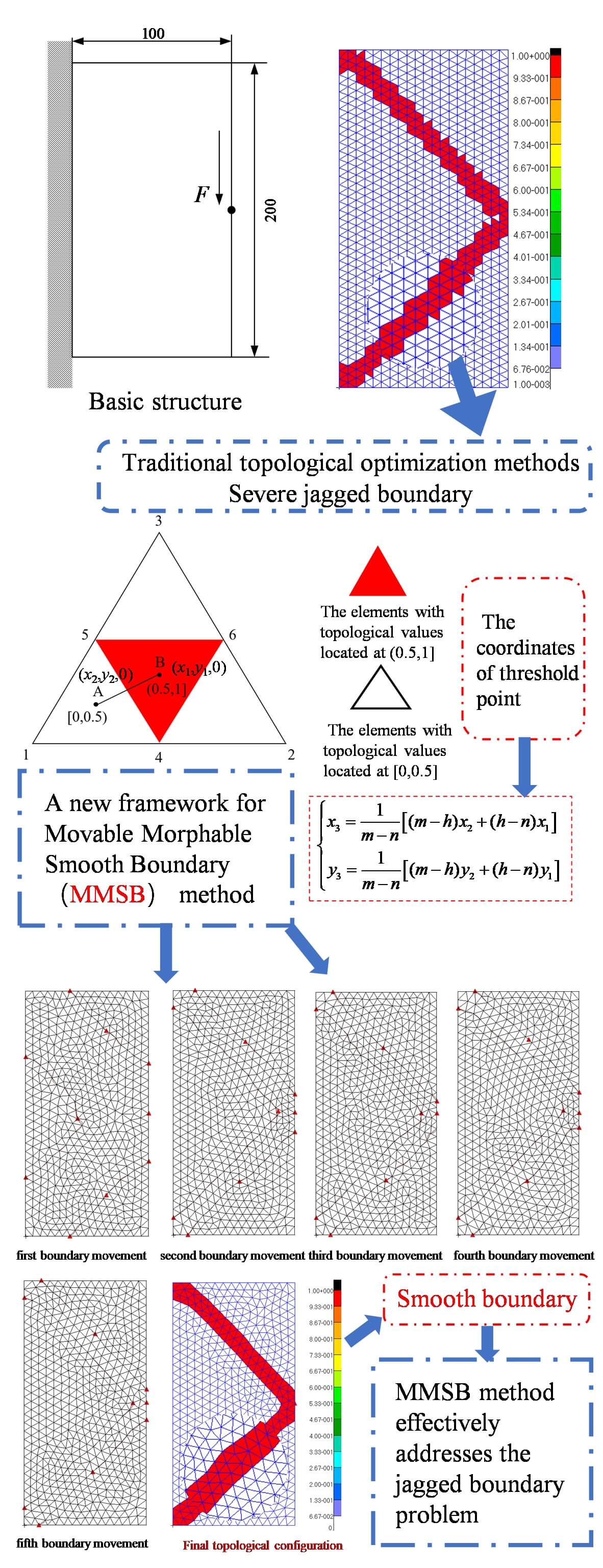
In previous topology optimization efforts utilizing the ICM method, a quadrilateral mesh usually served as the base mesh, often resulting in jagged boundaries that hinder manufacturability. The ICM topology optimization relies on finite element analysis, where meshing is crucial, as each element functions as a topological variable. Mesh delineation involves converting the physical model into a mathematical representation, and traditional quadrilateral meshing tends to exacerbate the issue of jagged boundaries. Therefore, employing a free mesh delineation approach, typically using triangular elements, presents a viable alternative.

This study proposes a novel topology optimization method known as Movable Morphable Smooth Boundary (MMSB), which primarily utilizes the triangle mesh as the base mesh due to its inherent flexibility and ease of deformation. The specific steps of the method are illustrated in the flow chart presented in Fig. 1. Initially, the triangle elements are treated as topology variables, with a threshold value, h, to be set as 0.5. With a Patran Command Language (PCL) program subscribed to the MSC. Patran & Nastran software, elements whose topology variables exceed the threshold are identified, and then common edges between these elements are checked. If a common edge is found, an interpolation method is applied to create threshold points based on individual elements. Then, the number of these threshold points is adjusted to ensure continuity. The Loft multipoint curve in the spline curve method is then utilized to connect the points, forming a curve that represents the contour corresponding to the threshold value of 0.5. Finally, the mesh is redrawn along this contour.

Figure 1: Flowchart of the Moving Morphable Smooth Boundary (MMSB) method

The whole optimization process is shown in Fig. 2, with six main steps. First, establish the initial finite element model, determine the geometric parameters of the model (length, width, thickness), material parameters (Poisson’s ratio, modulus of elasticity), mesh element size, displacement boundary conditions, and load boundary conditions; second, set the optimization parameters, which mainly include the value of the displacement constraints and the accuracy of the convergence; third, use the ICM topology optimization method combined with the finite element analysis to perform the optimization iteration and structural analysis; Fourth, determine whether the optimization iteration to the fourth step, if the iteration to the fourth step to find the threshold h value of 0.5 contour and along the curve for the mesh re-division, which is the first time the boundary line; Fifth, on the basis of a new round of finite element structural analysis and optimization iteration; Sixth, the number of iterations in the second optimization iteration is increased by four steps on the basis of the first optimization, to observe whether the boundary is smooth and similar to the first boundary, if similar and smooth to meet the convergence that is the end of the iteration, and output the topological map.

Figure 2: Overall optimization flow chart

3.2 Threshold Point

Since the topology optimization needs to be operated by the finite element method, it needs to be applied to the finite element software platform for the study, and this study mainly uses the PCL language in the MSC. Patran and Nastran software for the study. The study of the Movable Morphable Smooth Boundary method mainly involves the selection of threshold points because only by finding the corresponding threshold points can the connection of curves be achieved to form the contour and ultimately realize the smoothness of the boundary.

Threshold points are selected as shown in Fig. 3. The red triangular elements represent the elements with topological values located at [0.5, 1], and the white triangular grids represent the elements with topological values located at [0, 0.5]. Points A and B represent the center of the two grids, and the topological value of the point is the topological value of the element. The topological value of the point is the topological value of the element, and the topological value of the point is interpolated using interpolation to find the threshold point between the line segments AB, and the default threshold point is 0.5.

Figure 3: Introduction to the threshold points of the triangular mesh

The coordinates of the threshold point are mainly found using interpolation. Assume that the point whose topological value is greater than 0.5 is B(x1, y1, 0), and the point whose topological value is less than 0.5 is A(x2, y2, 0). Then, the coordinates of a point between these two points are expressed as follows:

{x3=1m−n[(m−h)x2+(h−n)x1]y3=1m−n[(m−h)y2+(h−n)y1](27)

where h is a threshold value; m is a topology value that is greater than or equal to the threshold value; n is a topology value that is less than the threshold value. Thus n < h < m.

4  Numerical Examples

4.1 Numerical Example 1

Example 1: The planar body base structure shown in Fig. 4 has dimensions of 100 × 200 × 6 mm, the finite element model is shown in Fig. 5. The modulus of elasticity of the material is 68.89 GPa, Poisson’s ratio is 0.3, and the centralized load F = 15.6 kN acts on the midpoint of the right boundary, and the left boundary is fixed constraint. The displacement constraint is that the vertical downward displacement of the loaded point is less than or equal to 0.5 mm. The mesh is a three-node triangular element.

Figure 4: Basic structure

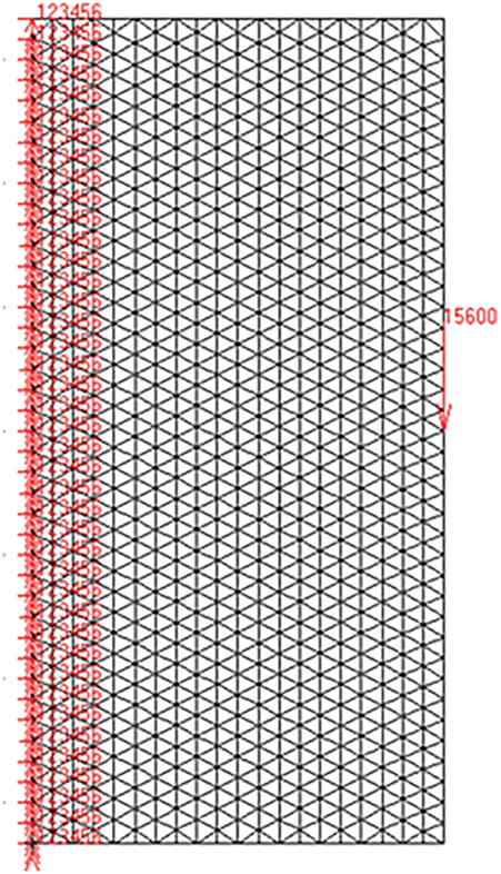
Figure 5: Finite element model

The final topological configuration is shown in Fig. 6 without using the Movable Morphable Smooth Boundary (MMSB) topology optimization method, and after inversion is shown in Fig. 7, and the weight and displacement curves of the structure after inversion are shown in Figs. 8 and 9. The mesh re-division is conducted to obtain the boundary shifting diagram, as shown in Fig. 10. There is almost no change from the fourth time when the fifth boundary shifting is conducted. The boundary smoothness is more obvious, so the convergence condition is reached after the fifth boundary shifting, and the final topological configuration is shown in Fig. 11.

Figure 6: Topological figure without Moving Morphable Smooth Boundary method

Figure 7: Topological configuration after inversion

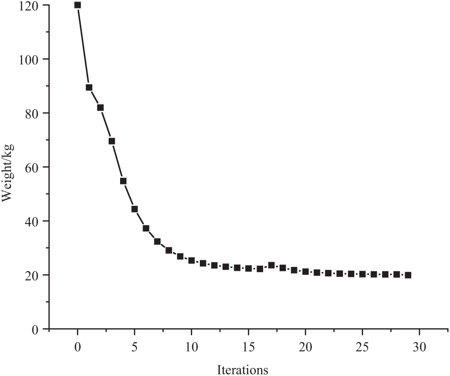
Figure 8: Weight iteration curve after inversion of conventional optimization for calculation example 1

Figure 9: Displacement iteration curve after inversion of conventional optimization for calculation example 1

Figure 10: Five boundary shifts

Figure 11: Final topological configuration of the MMSB approach

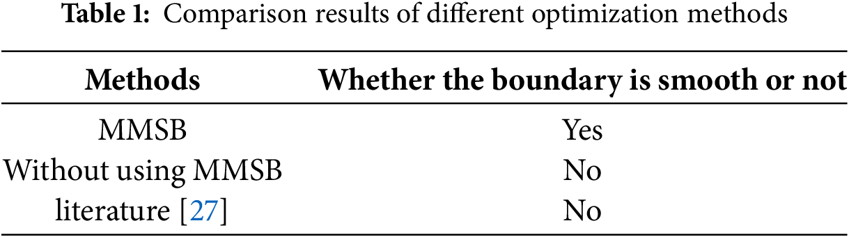
The final topological configuration obtained in the literature [27] using a traditional quadrilateral mesh is shown in Fig. 12. The five boundary movement changes in example 1 indicate that the boundary of the fifth time is relatively smooth. There is almost no change with the topological configuration of the fourth time so that the convergence condition can be reached. The weight iteration curve obtained from the five boundaries is shown in Fig. 13, and the final converged weight is 22.5 kg. Comparing the results of the method without Movable Morphable Smooth Boundary (MMSB) and the results of the method, as listed in Table 1, indicates that the boundary using the MMSB method is smooth enough to facilitate direct manufacturing at a later stage. The boundary using the MMSB method is smooth enough to facilitate direct fabrication at a later stage.

Figure 12: Traditional optimization results from the literature [27]

Figure 13: Five iterative curves for the weight of the MMSB

4.2 4.2 Numerical Example 2

Example 2: The base structure shown in Fig. 14 is 520 × 260 × 6 mm, and to reduce the computational amount of the symmetric structure is used for the analysis, its symmetric base structure is shown in Fig. 15, and the finite element model is illustrated in Fig. 16. The modulus of elasticity of the material is 68.89 GPa, Poisson’s ratio is 0.3, and the centralized load P = 21 kN acts at the midpoint of the lower boundary, and the structure is hinged at the lower left corner and simply supported at the lower right corner. The displacement constraint is that the vertical downward displacement of the loaded point is less than or equal to 0.8 mm.

Figure 14: Basic structure

Figure 15: Symmetrical basic structure

Figure 16: Example 2 Finite element model

A total of eight boundary shifts in Example 2 are performed using the MMSB method, and after the eighth boundary shift, the boundary shift is more similar to the seventh boundary shift, and the overall boundary of the eighth shift is smoother so that the conditions for convergence can be achieved. The topology graph with a smooth boundary containing only 0–1 is finally obtained, and the iterative curves of the weight of the structure with eight boundary shifts are shown in Fig. 17. The weight of the structure is 101.4 kg after the final convergence, and the topology graph with smoother boundary is illustrated in Fig. 18. The mesh re-division is conducted to obtain the boundary shifting diagram as shown in Fig. 19.

Figure 17: Eight iterative curves for weight of Movable Morphable Smooth Boundary

Figure 18: Final topological configuration of the MMSB method in example 2

Figure 19: Eight boundary shifts

Since the example uses a symmetric structure, the overall weight of the structure should be doubled for the original structure. The results obtained by optimizing the traditional topology and the results obtained using the MMSB method using mirror symmetry are shown in Figs. 20 and 21, respectively, and the results based on the quadrilateral mesh in the literature [27] are depicted in Fig. 22. The topology diagrams obtained by comparing the three approaches demonstrate that the topological configurations obtained by using the triangular mesh but not using the MMSB method are different from the results obtained by using the MMSB method as well as based on the results obtained by using the quadrilateral mesh in the literature [28], which is attributed to the existence of laziness in the mesh. However, it can be appropriately ignored. The results obtained from the three methods are compared as listed in Table 2, where the weight of the structure is the overall structural mass after mirroring. The results obtained by using the MMSB method are smoother, which is favorable for direct fabrication at a later stage, and it also shows that the MMSB method is a very effective method to improve the jagged boundary.

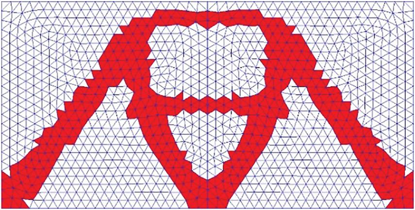
Figure 20: Symmetry diagram without MMSB method in example 2

Figure 21: Symmetry diagram of the MMSB method in example 2

Figure 22: Traditional optimization results from literature [28]

4.3 4.3 Numerical Example 3

Example 3: The base structure is depicted in Fig. 23, with basic dimensions of 80 × 50 × 1 mm, and its finite element model is shown in Fig. 24. The modulus of elasticity of the material is 1.0 × 106 MPa, and the Poisson’s ratio is 0.3, and a centralized load of F = 9000 N is applied to the lower-right corner of the model, and a fixed constraint supports the left boundary, and the displacement constraint is that the vertical downward displacement at the point of the load effect is less than or equal to 0.5 mm. The edge length of the element is set to 3 mm.

Figure 23: Basic structure of example 3

Figure 24: Finite element model of example 3

The inverse topology optimization configuration obtained without using the MMSB method is shown in Fig. 25, where the jagged boundary is more severe.

Figure 25: Topological configuration after inversion of example 3

A total of seven boundary shifts in Example 3 are performed using the MMSB method, and after the seventh boundary shift, the boundary shift was more similar to the sixth boundary shift, and the overall boundary is smoother in the seventh shift so that the convergence condition can be achieved. The mesh re-division is conducted to obtain the boundary shifting diagram as shown in Fig. 26. The final topological graph with smooth boundary containing only 0–1 is obtained as shown in Fig. 27. The final topological configuration of this algorithm obtained in the literature [29] using a quadrilateral based mesh is shown in Fig. 28. The structure weight iteration curves for seven boundary shifts obtained using the MMSB method are shown in Fig. 29. The final converged structure weight obtained is 1.65 kg.

Figure 26: Seven boundary shifts

Figure 27: Final topological configuration of the MMSB method in Example 3

Figure 28: Traditional optimization results from literature [29]

Figure 29: Seven iterative curves for weight of MMSB

The topological configurations obtained without using the MMSB topology optimization method, those in the literature [29], and those of the MMSB method are the same. The results obtained by the three methods, as listed in Table 3, do not differ much in terms of the weights of the structures. The results obtained using the MMSB method are smoother, indicating that the MMSB method is a very effective method to improve the jagged boundary.

5  Conclusion

This study develops a topology optimization model for weight minimization with multiple displacement constraints utilizing the ICM method. It uses the triangular meshing during the structural design optimization as the base mesh and achieves the boundary movement through contour redistribution of the mesh, resulting in an optimal topology with smooth boundaries. The Movable Morphable Smooth Boundary (MMSB) method effectively addresses the jagged boundary problem, and numerical examples demonstrate its effectiveness and feasibility.

However, the movable deformation boundary method requires multiple times of re-meshings, which limits computational efficiency. Future work will focus on enhancing the computational efficiency. In addition, the numerical examples provided are based on a two-dimensional model. If the Movable Morphable Smooth Boundary (MMSB) is to be extended to a three-dimensional model, it will require re-establishing three-dimensional boundary curves, increasing the complexity. This issue shall be addressed in future studies.

Acknowledgement: The authors would like to thank the School of Mathematics, Statistics and Mechanics, Beijing University of Technology, for providing the necessary facilities and resources for conducting this research.

Funding Statement: This work shown in this paper has been supported by the National Natural Science Foundation of China (Grant 12472113).

Author Contributions: The authors confirm their contribution to the paper as follows: study conception and design: Jiazheng Du, Hongling Ye; data collection: Ju Chen; analysis and interpretation of results: Ju Chen, Bing Lin, Zhichao Guo; draft manuscript preparation: Ju Chen. All authors reviewed the results and approved the final version of the manuscript.

Availability of Data and Materials: All data generated or analyzed during this study are included in this paper.

Ethics Approval: Not applicable.

Conflicts of Interest: The authors declare no conflicts of interest to report regarding the present study.

References

1. Zhu JH, Zhou H, Wang C, Zhou L, Yuan SQ, Zhang WH. Current and future development of topology optimization technology for additive manufacturing. Aerospace Manufact Technol. 2020;63(10):24–38. doi:10.16080/j.issn1671-833x.2020.10.024. [Google Scholar] [CrossRef]

2. Liu BY, Wang XM, Yang G, Xing BD. Research progress on topology optimization design for metal additive manufacturing. China Laser. 2023;50(12):188–203. [Google Scholar]

3. Fu XJ. Integrated Optimized design of continuum structures. J Mech Eng. 2012;48(1):128–34. [Google Scholar]

4. Zhang GF, Xu L, Wang X, Xiao NX. Study on the post-processing method for topology optimization of continuum structures based on the variable density method. Mech Strength. 2022;44(4):845–51. doi:10.16579/j.issn.1001.9669.2022.04.013. [Google Scholar] [CrossRef]

5. Li Z, Lee T, Yao Y, Xie YM. Smoothing topology optimization results using pre-built lookup tables. Adv Eng Softw. 2022;173(12):103204. doi:10.1016/j.advengsoft.2022.103204. [Google Scholar] [CrossRef]

6. Liu HL, Wang PJ, Liang Y, Long K, Yang DX. Topology optimization for harmonic excitation structures with minimum length scale control using the discrete variable method. Comput Model Eng Sci. 2023;135(3):1941–64. doi:10.32604/cmes.2023.024921. [Google Scholar] [CrossRef]

7. Maute K, Ramm E. Adaptive topology optimization. Struct Optim. 1995;10(2):100–12. doi:10.1007/BF01743537. [Google Scholar] [CrossRef]

8. Thomás YSH, Ivan FMM, Anderson P. A simple adaptive mesh refinement scheme for topology optimization using polygonal meshes. J Braz Soc Mech Sci Eng. 2018;40(7):1–17. doi:10.1007/s40430-018-1267-5. [Google Scholar] [CrossRef]

9. Da DC, Xia L, Li GY, Huang XD. Evolutionary topology optimization of continuum structures with smooth boundary representation. Struct Multidiscipl Optim. 2018;57(6):2143–59. doi:10.1007/s00158-017-1846-6. [Google Scholar] [CrossRef]

10. Liu BS, Guo D, Jiang C, Li GY, Huang XD. Stress optimization of smooth continuum structures based on the distortion strain energy density. Comput Methods Appl Mech Eng. 2019;343(14):276–96. doi:10.1016/j.cma.2018.08.031. [Google Scholar] [CrossRef]

11. Muayad H, Majid MR. Plastic-limit probabilistic structural topology optimization of steel beams. Appl Math Model. 2024;128:347–69. doi:10.1016/j.apm.2024.01.029. [Google Scholar] [CrossRef]

12. Gómez-Silva F, Zaera R, Ortigosa R, Martínez-Frutos J. Topology optimization of lattice structures for target band gaps with optimum volume fraction via Bloch-Floquet theory. Comput Struct. 2025;307:107601. doi:10.1016/j.compstruc.2024.107601. [Google Scholar] [CrossRef]

13. Fu YF, Rolfe B, Chiu LNS, Wang YA, Huang XD, Ghabraie K. Smooth topological design of 3D continuum structures using elemental volume fractions. Comput Struct. 2020;231(2):106–213. doi:10.1016/j.advengsoft.2020.102921. [Google Scholar] [CrossRef]

14. Yu CT. MMC topology optimization method based on smoothing technique [MA thesis]. Dalian, China: Dalian University of Technology; 2021. [Google Scholar]

15. Huang MC, Du ZL, Liu C, Zheng YG, Cui TC, Mei Y, et al. Problem-independent machine learning (PIML)-based topology optimization—a universal approach. Extreme Mech Lett. 2022;56:101887. doi:10.1016/j.eml.2022.101887. [Google Scholar] [CrossRef]

16. Sui YK, Yang DQ. A new method for structural topological optimization based on the concept of independent continuous variables and smooth model. Acta Mech Sin. 1998;18(2):179–85. doi:10.1007/bf02487752. [Google Scholar] [CrossRef]

17. Peng XR, Sui YK. Topology optimization of continuum structures under forced harmonic vibrations. J Solid Mech. 2008;29(2):157–62. doi:10.1016/b978-0-12-812655-4.00008-0. [Google Scholar] [CrossRef]

18. Peng XR, Sui YK. First-order approximation of internal forces for stress-constrained topology optimization. Mech Strength. 2016;38(05):990–5. [Google Scholar]

19. Peng XR, Sui YK. Topological optimization of continuum structures under static displacement and frequency constraints by ICM method. J Computat Mech. 2006;23(04):391–6. [Google Scholar]

20. Long K, Zuo ZX. A hybrid modeling approach for ICM topology optimization based on different filter functions. Chinese Mech Eng. 2007;18(19):2303–6. [Google Scholar]

21. Long K, Zuo ZX. Nodal ICM topology optimization method under spatially independent interpolation. Eng Mech. 2010;27(12):90–95, 101. [Google Scholar]

22. Long K, Zuo ZX. Continuum topology optimization under harmonic response. Chinese Mech Engg. 2007;18(13):1556–9. [Google Scholar]

23. Yan JS, Sun PW, Ma ZK, Zhao XX, Dong XH. Effect of different parameters of power function filtering function on the convergence rate of topology optimization of laminates. Compos Mat Sci Eng. 2022;6:5–9. [Google Scholar]

24. Du JZ, Cong X, Zhang Y. Topology optimization of strength-safe continuum structures considering random damage. Comput Model Eng Sci. 2023;136(2):1091–120. doi:10.32604/cmes.2023.025585. [Google Scholar] [CrossRef]

25. Du JZ, Chen J, Li GM. Influence of filter functions on efficiency of topology optimization and gray-scale element. J Beijing Univ Technol. 2025;51(5):523–38. doi:10.11936/bjutxb2023070001. [Google Scholar] [CrossRef]

26. Sui YK, Ye HL. Continuum topology optimization methods ICM. Beijing, China: Science Press; 2013. 22 p. [Google Scholar]

27. Du JZ, Zhang Y, Meng FW. Fail-safe topology optimization of continuum structures with multiple constraints based on ICM method. Comput Model Eng Sci. 2021;129(2):661–87. doi:10.32604/cmes.2021.017580. [Google Scholar] [CrossRef]

28. Ye HL. Static topology optimization method and software development for continuum structures [Ph.D. Thesis]. Beijing, China: Beijing University of Technology; 2005. [Google Scholar]

29. Sui YK, Peng XR. Improvement of ICM methods for structural topology optimization. J Mech. 2005;37(2):190–8. doi:10.6052/0459-1879-2005-2-2004-286. [Google Scholar] [CrossRef]