
 Submit a Paper
 Propose a Special lssue
 Open Access
ARTICLE

A Hybrid LSTM-Single Candidate Optimizer Model for Short-Term Wind Power Prediction
1 Department of Information Technologies, Bilecik Seyh Edebali University, Bilecik, 11100, Turkey
2 Department of Electrical Electronics Engineering, Bilecik Seyh Edebali University, Bilecik, 11100, Turkey
3 Department of Computer Engineering, Bilecik Seyh Edebali University, Bilecik, 11100, Turkey
* Corresponding Author: Mehmet Balci. Email:
(This article belongs to the Special Issue: Advanced Artificial Intelligence and Machine Learning Methods Applied to Energy Systems)
Computer Modeling in Engineering & Sciences 2025, 144(1), 945-968. https://doi.org/10.32604/cmes.2025.067851
Received 14 May 2025; Accepted 03 July 2025; Issue published 31 July 2025
 View Full Text
 Download PDF
Abstract
Accurate prediction of wind energy plays a vital role in maintaining grid stability and supporting the broader shift toward renewable energy systems. Nevertheless, the inherently variable nature of wind and the intricacy of high-dimensional datasets pose major obstacles to reliable forecasting. To address these difficulties, this study presents an innovative hybrid method for short-term wind power prediction by combining a Long Short-Term Memory (LSTM) network with a Single Candidate Optimizer (SCO) algorithm. In contrast to conventional techniques that rely on random parameter initialization, the proposed LSTM-SCO framework leverages the distinctive capability of SCO to work with a single candidate solution, thereby substantially reducing the computational overhead compared to traditional population-based metaheuristics. The performance of the model was benchmarked against various classical and deep learning models across datasets from three geographically diverse sites, using multiple evaluation metrics. Experimental findings demonstrate that the SCO-optimized model enhances prediction accuracy by up to over standard LSTM implementations.Graphic Abstract
Keywords
Reducing carbon dioxide emissions has become a remarkable objective in attaining the sustainable development goals endorsed by United Nations members. A swift transition away from fossil fuels, which are a notorious contributor to climate change, is imperative to realize these objectives. Globally, coal, a non-renewable and environmentally detrimental fossil fuel source, represents 36.81% of the electrical energy generation [1]. The well-established impacts of fossil fuels include their cause of the greenhouse effect, exacerbation of climate change, and their finite nature. There is a growing need to promote sustainability in energy production and to mitigate the adverse environmental impacts of fossil fuels. Renewable energy sources, recognized as clean energy alternatives, are increasingly gaining popularity and warrant further promotion [2,3]. In 2021, the International Energy Agency (IEA) introduced the “Net Emissions Blueprint 2050,” outlining wind power as the leading contributor to the global electricity generation portfolio by 2050, projected to reach 35%. Despite the widespread production disruptions induced by the COVID-19 pandemic, global wind power installations stood at 95.3 GW in 2020, 93.6 GW in 2021, 77.6 GW in 2022, 116.6 GW in 2023, and 117 GW in 2024, marking substantial increases compared to previous years. These statistics, as reported in Global Wind Report 2024 by the Global Wind Energy Council (GWEC), underscore the remarkable global growth trajectory of wind energy deployment [4]. Wind energy, recognized as a sustainable and environmentally friendly power source, offers significant potential for mitigating the adverse environmental impacts linked to intensive energy use and emissions from coal-based electricity generation. Nevertheless, the inherent variability and intermittency of wind poses operational challenges for power systems, particularly in areas such as unit commitment and day-ahead generation planning [5]. Advancements in the precision of renewable energy forecasting can play a critical role in minimizing the likelihood of power system disruptions [6].
Wind speed forecasting models are generally categorized into four groups according to their prediction timeframes: very short-term, short-term, medium-term, and long-term. Very short-term predictions, ranging from a few seconds to 30 min, are primarily applied in real-time turbine control and load-following operations. Short-term forecasts, which span from 30 min to 6 h, are essential for effective load-dispatch planning. Medium-term forecasts, typically between 6 and 24 h ahead, support the scheduling of conventional power plants and enable strategic energy market participation. Long-term forecasts, which may cover periods from one day to one week or more, are critical for optimizing unit commitment processes [7].
Some studies on wind power forecasting have focused on predicting wind speed rather than power output [8–10]. Although wind speed forecasts may be suitable for certain applications, it is essential to recognize that grid operations and trading decisions require power forecasts. Converting wind speed into wind power involves a complex and nonlinear process, meaning that models demonstrating proficiency in wind speed prediction may not necessarily perform as well when forecasting power. Similarly, studies using wind speed datasets to simulate power values via a power curve may not accurately represent the actual variability observed in the operational power data [11]. Accessible wind power datasets [12] now enable the evaluation of models using power data, aligning more closely with the research objectives.
Wind power forecasting models can be categorized into three main methods: physical modeling, statistical approaches, and artificial intelligence (AI) techniques [13]. Physical models may utilize numerical weather predictions [14] or weather research and forecasting [15] to acquire forthcoming meteorological data. Consequently, the wind power can be computed using a wind power curve model that employs future meteorological data [16]. Nonetheless, the accuracy of wind power forecasting is contingent on the site-specific nature and reliability of the predicted meteorological data. Statistical methods, including autoregressive moving average (ARMA) [17] and seasonal autoregressive integrated moving average (SARIMA) [18], depend solely on historical data and employ statistical models to identify linear connections within smoothed wind-power datasets. Liu et al. [18] proposed a SARIMA model to forecast hourly-measured wind speeds in the coastal/offshore area of Scotland. Similarly, Singh and Mohapatra [19] found in their experiments that ARIMA tends to yield less-precise forecasts for high-frequency subseries. Nonetheless, in situations characterized by substantial meteorological shifts near the wind turbine or the presence of strong nonlinear relationships within the wind power data, the forecasting accuracy of statistical fitting methods often decreases.
Recently, many scholars have actively engaged in researching wind power methods driven by AI. As computational capabilities advance, AI techniques, such as machine learning and deep learning, are increasingly utilized in wind power forecasting and similar tasks involving forecasting multiple variables over time series data. Machine learning approaches have indicated superior performance, such as extreme learning machine (ELM) [20], support vector machine (SVM) [21], artificial neural network [22], kernel ELM [23], multi-layer perceptron [24]. Recent advancements in deep learning have introduced recurrent neural networks (RNNs), which exhibit remarkable efficiency in handling time-series data by effectively capturing historical data. However, prolonged forecasting periods frequently encounter challenges, such as vanishing and exploding gradients. To overcome these issues, researchers have proposed solutions, including long short-term memory (LSTM) [25], bidirectional LSTM (BiLSTM) [26], deep belief networks [27] and gated recurrent units (GRU) [28].
In recent years, large language models (LLMs), particularly those based on transformer architectures, have demonstrated exceptional capabilities across a wide range of natural language processing tasks due to their powerful reasoning and generalization abilities. Building on this success, researchers have started exploring their potential in time-series forecasting applications, including wind speed and power prediction. Unlike traditional statistical or machine-learning models, LLMs can encode higher-level semantic patterns and leverage prompt-based learning to interpret complex temporal dynamics. Two main strategies have emerged in this context: intra-modal transfer learning, where LLMs are fine-tuned directly on time-series data, and cross-modal knowledge transfer, where time-series inputs are transformed into textual prompts to utilize frozen LLMs without architectural modification. Recent studies such as GPT4TS and PromptCast have applied these paradigms to various forecasting tasks with promising results [29,30]. Specifically, for wind-power forecasting, cross-modal approaches offer a compelling alternative by avoiding computationally expensive fine-tuning and mitigating overfitting risks on small datasets. While LLM-based models have shown notable improvements over traditional forecasting methods, research in this area is still in its early stages, and further efforts are needed to adapt these models effectively to domain-specific requirements.
There has been a noticeable shift towards employing hybrid structures for deep learning and machine learning techniques in wind power forecasting. This trend aims to address the shortcomings of standalone models, while leveraging the unique strengths of both approaches. Hybrid models created by integrating metaheuristic approaches into AI methods and incorporating pre-processing via decomposition methods are becoming increasingly prevalent. Meta-heuristic optimization algorithms are extensively utilized in forecasting wind power and speed. However, a thorough review of the literature reveals several notable shortcomings and challenges. Presently, meta-heuristic based hybrid algorithms are primarily applied to predict the power output of individual wind farms; however, the datasets from these farms are often insufficient in size to qualify as big data. However, with the continual growth in the installed wind power capacity, dataset sizes are expanding significantly, paving the way for the potential accumulation of big data in this domain. Using an optimized deep learning model, Ewees et al. [31] proposed a new wind power forecasting approach based on a heap-based optimizer (HBO). To boost the efficiency of LSTM-based forecasting, some approaches incorporate metaheuristic optimizers, such as HBO, to fine-tune the model parameters, yielding significant accuracy gains. However, the proposed model may cause convergence speed problems. Altan et al. [32] developed LSTM network and decomposition methods with grey wolf optimizer (GWO). To achieve a more accurate prediction model, the GWO algorithm was applied to optimize the contribution of each decomposed subcomponent of the original signal. Their results showed that the decomposition-based LSTM-GWO hybrid model was superior to all the implemented models. Similarly, hybrid approaches such as the Lévy flight Chaotic Whale Optimization algorithm (LCWOA)-ELM model [33], Swarm Decomposition-Meta-ELM (SWD-Meta-ELM) [34], and improved quantum particle swarm optimization algorithm (QPSO)-based combined model [35] GWO-based complete ensemble empirical mode decomposition with adaptive noise (CEEMDAN)-convolutional neural network (CNN)-BiLSTM [36] have been proposed for wind-power forecasting. An adaptive forecasting model based on GWO-LSTM was proposed in [37]. Medium- and long-term forecasting were investigated by considering different wind energy characteristics. However, their model performances were compared only with those of the LSTM-based models. Although AI-based hybrid models combine advantages through metaheuristic approaches, there is no single dominant model. Currently, various regional studies are underway to explore the characteristics of diverse wind speeds. Furthermore, evaluating model performance across multiple regions by testing on datasets enhances their reliability. The optimal determination of deep learning method parameters, such as LSTM, significantly affects the model performance. Despite the effective use of meta-heuristic algorithms to improve the optimization performance of deep learning models, they frequently suffer from problems, such as early convergence, local optima stagnation, and overfitting. Hence, there is a need to investigate novel metaheuristic algorithms capable of overcoming these obstacles. Among meta-heuristic approaches, the Single Candidate Optimizer (SCO) has recently attracted significant interest because of its inventive approach and encouraging outcomes, which are characterized by notably diminished computation costs and memory demands [38]. Research indicates that SCO demonstrates faster convergence to optimal solutions than alternative algorithms [39]. Nonetheless, the effectiveness of SCO is contingent upon the nature of the problem and requires further investigation, particularly for near-real-time applications. Moreover, there is investigation to suggest that this algorithm holds promise for integration with other meta-heuristics and forecasting tools [39]. In this study, the literature reviewed on wind power and wind speed is presented in Table 1.

This paper proposes a novel hybrid model for wind power forecasting that combines LSTM networks with the SCO algorithm. The uniqueness of the approach lies in SCO’s single-solution-based search mechanism, which contrasts with traditional population-based optimization methods commonly used in similar models. Unlike conventional LSTM models, where the parameters are initialized randomly, the proposed method utilizes SCO to determine the optimal initial weights and biases, which are then fine-tuned using the Adam optimizer. This hybrid strategy enhances the convergence speed while reducing the computational complexity and improving the forecasting accuracy. To evaluate its effectiveness, the model was tested using one-year real-world hourly offshore wind data from three geographically diverse wind farms in the United Kingdom and Denmark. Comparative experiments against benchmark models, including standard LSTM, BiLSTM, ANFIS, MLP, ELM, and TR-Net, were conducted using multiple performance metrics. The results show that the LSTM-SCO model outperforms existing methods in terms of both accuracy and efficiency. A key strength of the proposed model is its robustness across datasets with varying geographical characteristics, which highlights its scalability and wide applicability. The model demonstrates strong potential for real-time forecasting in critical areas, such as grid management, energy planning, and renewable integration, offering practical value for both academic and industrial applications.
The following sections of this paper are arranged accordingly: Section 2 describes the methodology, encompassing the LSTM model, SCO algorithm, datasets, and performance metrics. The comparative wind-power forecasting results and discussion are presented in Section 3. The final section presents the results of the proposed model and provides an outlook for future studies.
2.1 Long-Short Term Memory Model
The Long Short-Term Memory (LSTM) architecture is a type of artificial neural network widely employed in deep learning tasks. It is particularly effective in handling time-dependent data and is capable of learning long-range temporal patterns. Unlike traditional Recurrent Neural Networks (RNNs), LSTM models offer improved performance by addressing the vanishing gradient problem. As a result, LSTM has become a widely adopted model, particularly in fields such as natural language processing, speech recognition, and machine translation. Its ability to achieve highly accurate and robust results on complex and large-scale datasets has contributed to its popularity [40]. Structurally, the LSTM network includes key components responsible for managing the input data, updating the cell state, and generating the outputs. Below is a basic description of the mathematical structure of the LSTM.
1. Inputs: The input sequence of the LSTM begins with
2. Gates: The LSTM model includes three gates, namely the forget gate, input gate, and output gate.
The Forget Gate (
where W and U represent the weights of the input and recurrent connections, the subscript
3. Cell State (
Furthermore, learning was performed using the output of the forget gate
Here,
4. Output Gate (
Here,
The steps described above were repeated iteratively. The model optimizes the weight (W) and bias (b) parameters to reduce the error between the LSTM outputs and actual training data. By optimizing these parameters, the model improved its ability to match the predicted results with actual observations, thereby achieving higher precision during the training phase.
2.2 Single Candidate Optimization Algorithm
Balancing exploration and exploitation remains a critical challenge in metaheuristic optimization research. Traditional population-based algorithms rely on multiple agents to explore the search space, which often leads to high computational costs and complex coordination. The Single Candidate Optimization (SCO) algorithm diverges from this convention by focusing on a singular candidate solution [39]. Through a two-phase strategy, SCO enhances search efficiency and avoids local optima by dynamically adjusting the position of the candidate [38]. This innovative approach allows the algorithm to effectively adapt to various optimization landscapes. The position-update mechanism in the initial phase is governed by the following equation:
In this equation,
Here,
In this formulation,
2.3 The Proposed Hybrid Model Approach: LSTM-SCO
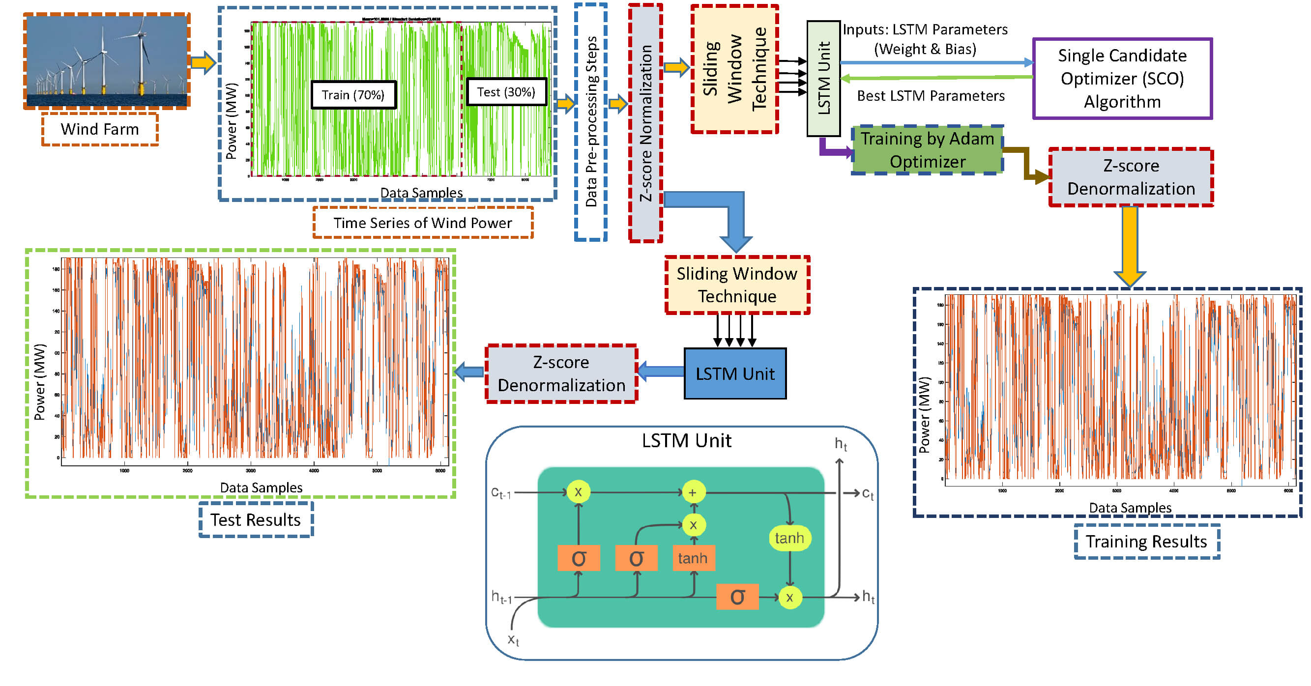
This subsection provides a detailed explanation of the architecture of the proposed LSTM-SCO model. In conventional LSTM models, the weight parameters are randomly initialized and subsequently optimized using the Adam algorithm during training. However, in the proposed method, the initial parameter values are determined using the SCO algorithm, thereby highlighting the importance of proper initialization in addressing optimization problems. Subsequently, the parameters were further refined using the Adam optimizer. The overall framework of the proposed model is depicted in Fig.1 and general operational steps of the model are outlined below.
1. The dataset to be used is selected.
2. The first 70% of the dataset is used for the training phase of the model, while the remaining 30% is used for the testing phase. The data used in the models were not selected randomly; instead, the fixed partitioning method was applied.
3. The data are normalized using the Z-score method.
4. The normalized data are used for inputs the LSTM model using the sliding window technique.
5. The training parameters of the LSTM are tuned using the Single Candidate Optimizer (SCO).
6. The LSTM model is trained using the Adam optimizer.
7. The results from the training phase are denormalized to obtain the final training outputs.
8. The data selected for the test phase are provided as input to the LSTM model.
9. The results obtained from the test phase are denormalized to produce the final testing outputs.
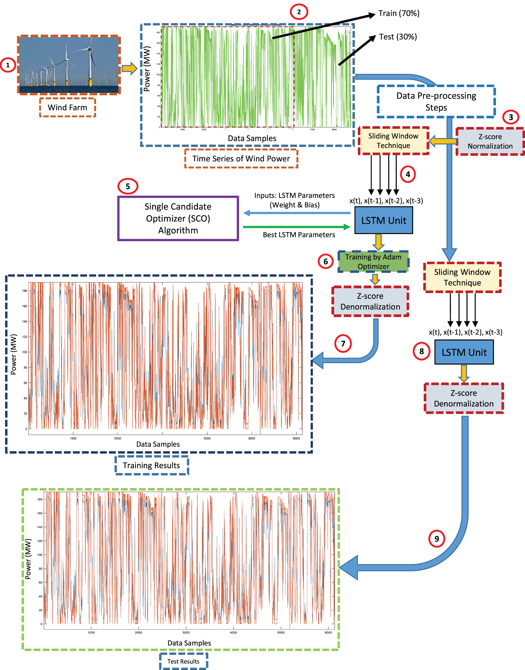
Figure 1: Diagram of LSTM-SCO hybrid model
A major advantage of applying the SCO algorithm to initialize the LSTM model parameters is its capability to process a single candidate solution. This leads to a notable reduction in the computation time compared with population-based metaheuristic techniques. The LSTM-SCO model functions according to the following sequential steps.
1. The dataset used in this study includes wind energy data gathered from three offshore sites. The measurements were recorded hourly over a one-year period, amounting to 8760 h of data. This extensive dataset captures variations in wind energy generation, enabling a thorough analysis of the performance and efficiency of the different prediction models.
2. The wind power time series was normalized using z-score normalization during the data preprocessing steps. Then, four input series (
3. The LSTM-SCO model was trained using 70% of the input and output time series obtained from the preprocessing steps, and the rest were used in the testing process.
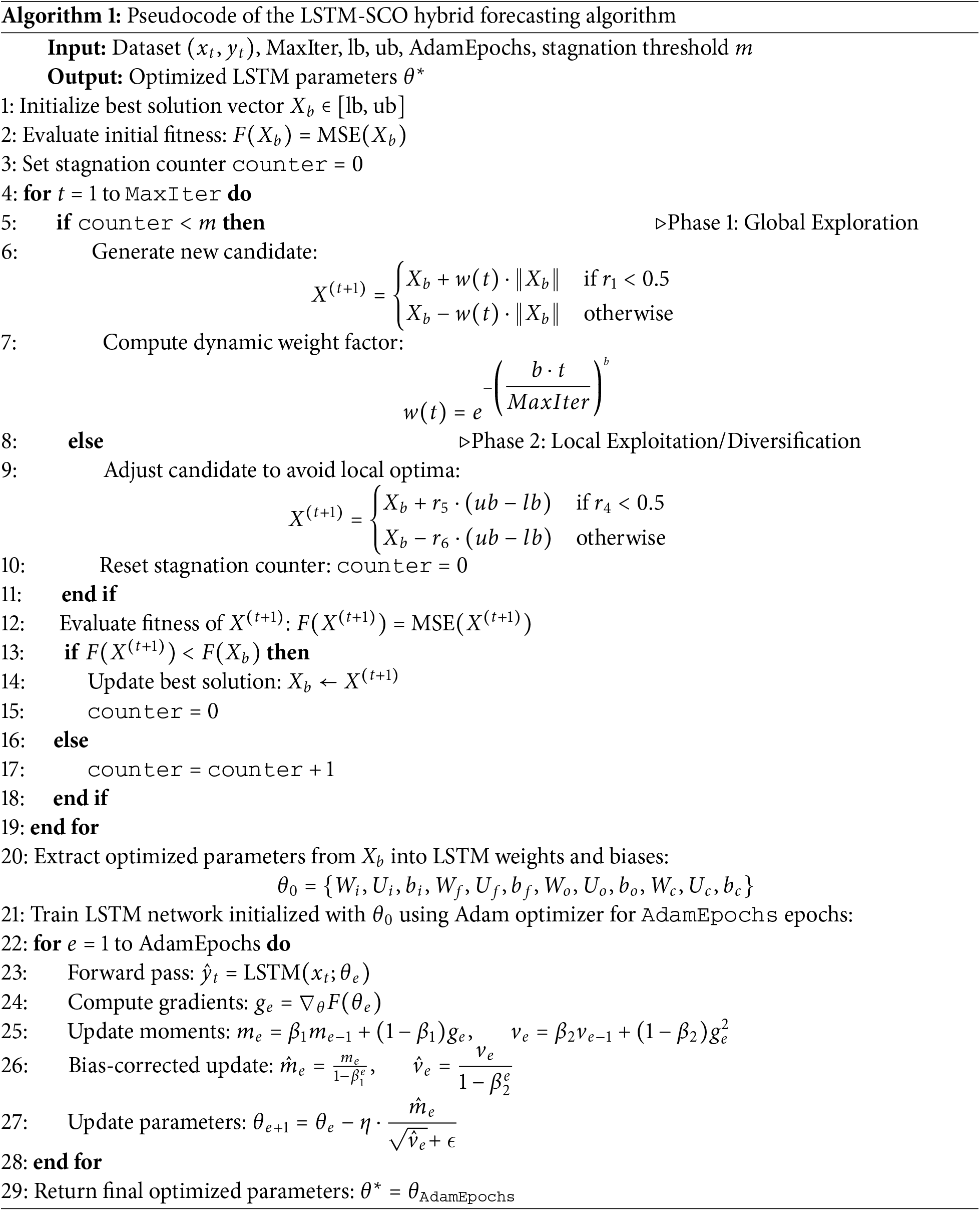
4. The LSTM model parameters are pre-trained with SCO for a short period (100 iterations) using the pre-processed dataset provided for training. In this phase, all trainable parameters of the LSTM network, including input-to-hidden weights (
where
After the SCO iteration completes, the best solution
Finally, these parameters are further fine-tuned using the Adam optimizer, which adaptively adjusts learning rates based on first and second moment estimates:
Here,
5. In the testing phase, the pre-trained LSTM-SCO model is tested on 30% of the dataset that was not included in the training stage. This helps to evaluate how well the model generalizes to new, unseen data. The effectiveness of the model was measured using the RMSE, MSE, MAE, and
To provide a clear and structured representation of the proposed LSTM-SCO hybrid model, we present the pseudocode of LSTM-SCO hybrid model in Algorithm 1. The procedure includes parameter vectorization, MSE-based fitness evaluation, SCO-based optimization, and subsequent refinement using the Adam optimizer.
To assess the predictive performance of the different models for wind power forecasting, four key evaluation metrics were utilized. These metrics collectively provide a thorough assessment of the forecasting accuracy. The Mean Squared Error (MSE) calculates the average of the squared discrepancies between the predicted and actual values and serves as an indicator of the overall prediction performance. The Root Mean Squared Error (RMSE), obtained by taking the square root of the MSE, expresses the error in the same unit as the target variable, making the interpretation more intuitive. The Mean Absolute Error (MAE) represents the mean of the absolute deviations between the predictions and observations, offering a straightforward measure of the average error magnitude. Finally, the coefficient of determination (
where
A comprehensive dataset comprising hourly wind energy outputs over a twelve-month period from three offshore wind farms served as the basis for training and testing the forecasting models. The wind farms include the West of Duddon Sands (Dataset 1) and Barrow (Dataset 2), which are located in the region between England and Ireland. Dataset 1 operates at 388.8 MW with a standard deviation of 72.08, and Dataset 2 had a capacity of 90 MW with a standard deviation of 28.15. The Horns Power wind farm (Dataset 3), situated off Denmark’s North Sea coast, has a capacity of 160 MW and standard deviation of 51.20.
3 Forecasting Results and Performance Evaluation
This section presents a comprehensive analysis of the forecasting results obtained from all the models evaluated, namely, the proposed LSTM-SCO model, Bi-LSTM, LSTM, MLP, ANFIS, ELM, and Transformer (TR-Net) models. According to prior findings, no single forecasting method consistently outperforms the others across all evaluation metrics for wind-power prediction [41]. To assess the effectiveness of the proposed model, the results were compared with those of several state-of-the-art and traditional models. Model performance was measured using evaluation metrics such as MSE, RMSE, MAE, MARE, MSRE, RMSPE, and
The hybrid LSTM-SCO model, along with other benchmark models, was executed on a personal computer with an Intel Core i5-7500 processor operating at 3.40 GHz, an Intel HD Graphics 630 GPU with 128 MB of memory, and 16 GB of RAM. The configurations for each model were as follows: both LSTM and BiLSTM models were designed with two hidden layers containing 100 neurons each, trained over 50 epochs with a mini-batch size of 16, utilizing the ‘Adam’ optimization algorithm. The MLP models employed ‘logsig’ and ‘tansig’ activation functions in conjunction with the ‘traingdm’ back-propagation training function. For the ANFIS model, two membership functions were assigned, with ‘grid partitioning’ adopted as the training method; ‘gaussmf’ was selected as the input membership function type, and a linear function was used for the output. The ELM model was configured with a single hidden layer containing eight neurons and an input feature size determined by the dataset. The activation function used was tanh and the solution type was set to Moore-Penrose (MP) for the output weight calculation. Random weight initialization was applied to the input layer as per the standard ELM approach. The Transformer model was implemented with four attention heads, three encoder layers, and model dimensions of 64. The model architecture included an input layer followed by a dense layer with 32 units, a transformer block with specified parameters, global average pooling, dropout layers, and final dense layers for regression. Both models were trained for 50 epochs using the Adam optimizer.
The SCO algorithm employs several critical parameters to enhance its search process: the maximum number of iterations, counter for monitoring fitness stagnation, number of consecutive unsuccessful attempts (m), number of function evaluations during the initial phase (
The convergence curves in Fig. 2 illustrate that the SCO algorithm successfully optimizes the initial parameters of the LSTM model, leading to faster and more stable convergence. This highlights the robustness of the SCO-based approach in achieving superior performance across all datasets.
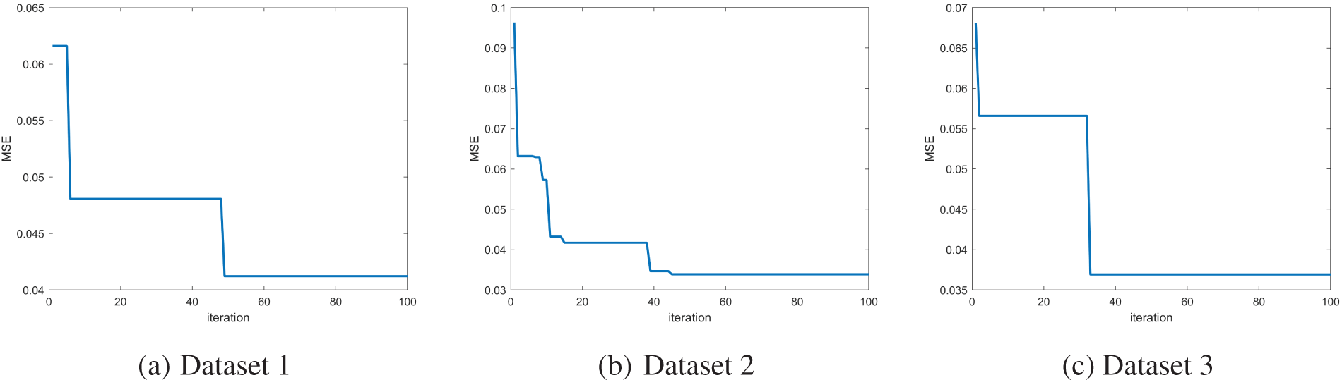
Figure 2: Convergence behavior of the SCO algorithm in LSTM parameter initialization across all datasets
3.1 Forecasting Results for Dataset 1
This section compares the one-hour-ahead power prediction results of the models for the training and test phases using one year of wind power data for the West of Duddon Sands area. Table 2 reports the outcomes from the training and testing phases utilizing various models such as LSTM, BiLSTM, LSTM-SCO, MLP, ANFIS, ELM, and TR-Net, on the Dataset 1. In particular, the LSTM-SCO model demonstrated superior performance during both the training and testing phases, achieving MSE values of 360.74 and 345.26, RMSE values of 18.993 and 18.581, and

Fig. 3 displays the forecasting outcomes of the models applied to the West of Duddon Sands dataset. Upon closer examination of the graph, the success of the models used within a zoomed window around the 1000th data point becomes evident as they closely track the target curve depicted in black. The LSTM-SCO model, represented by the purple curve, was the most successful, while the MLP model, indicated by the green curve, was observed to be the least successful. Furthermore, the curve of the BiLSTM model closely follows the target graph, establishing it as the second most successful model.
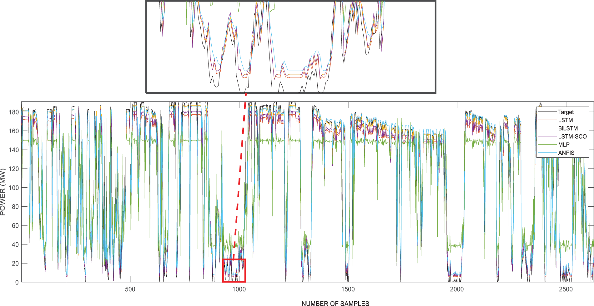
Figure 3: Results of using models for Dataset 1
The
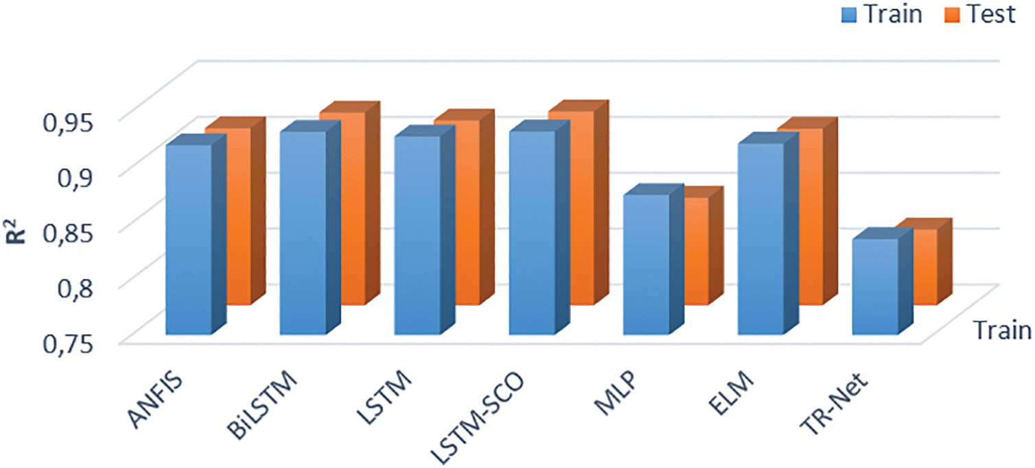
Figure 4:
3.2 Forecasting Results for Dataset 2
This section presents a comparative analysis of the proposed LSTM-SCO model applied to the Barrow dataset against the implemented models, accompanied by detailed analyses and discussions. The performance metric results for the LSTM, BiLSTM, LSTM-SCO, MLP, ANFIS, ELM, and TR-Net models obtained in both the training and testing stages using the dataset from the Barrow region in the UK are shown in Table 3.

As shown in the table, it is observed that during the training phase, the proposed hybrid LSTM-SCO model achieved the best forecasting results with the lowest MSE, RMSE, MAE, and
The forecasting test results of the implemented models for wind power Dataset 2 are illustrated in Fig. 5. The results indicate that all models, with the exception of MLP, successfully approximated the wind power trend during forecasting.
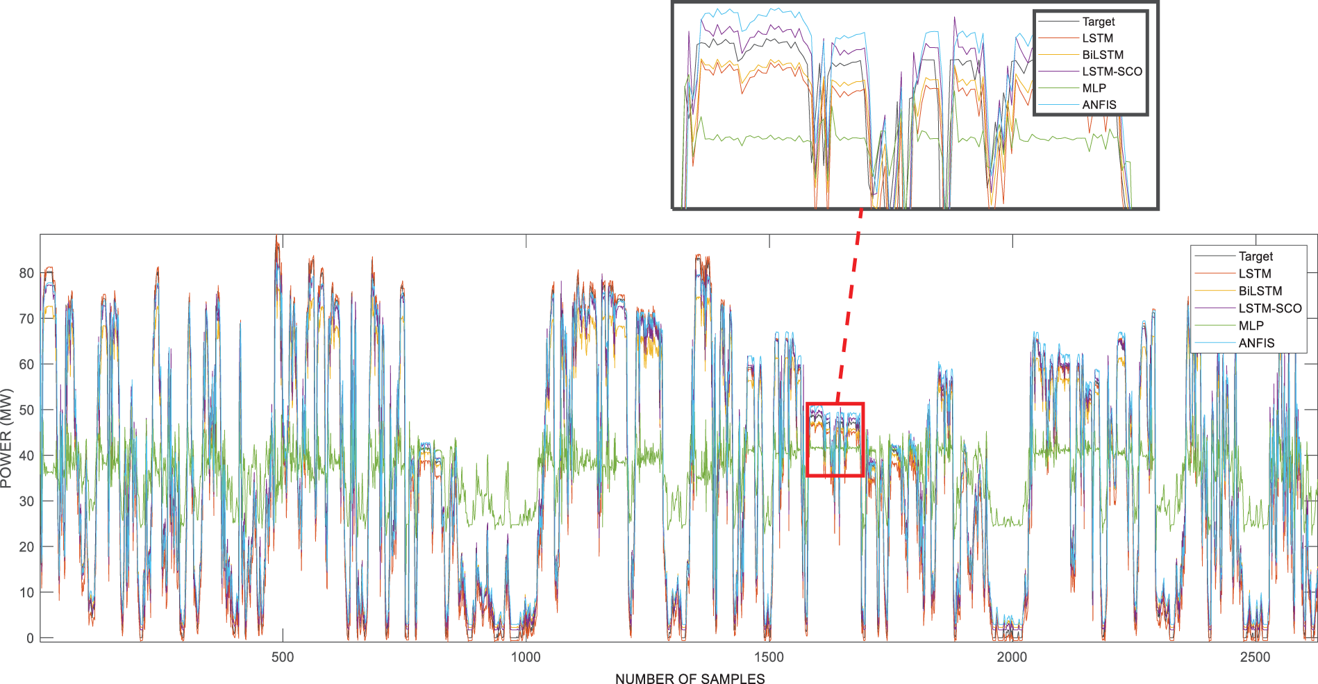
Figure 5: Results of using models for Dataset 2
The curve represented by the purple line, which is closest to the black target curve, corresponds to the LSTM-SCO model, as shown in the enlarged frame. The MLP model demonstrated limited capability in accurately capturing signal variations, especially during periods of rapid changes in wind power. When comparing the proposed model solely with the LSTM model, it becomes evident that the SCO metaheuristic approach significantly affects the model performance by optimizing the parameters. Throughout the training phase, the
The graphs that illustrate the
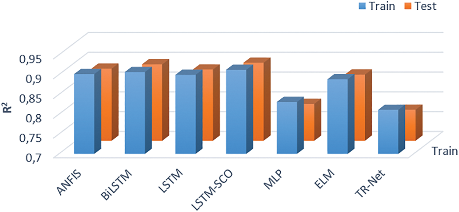
Figure 6:
3.3 Forecasting Results for Dataset 3
The models forecasted one-hour-ahead power using one year of wind power data from the Horns Power region in this subsection. The performance metric results for the training and testing phases of the proposed LSTM-SCO model and other models are detailed in Table 4.

Observing the values in the table, it is apparent that the proposed model exhibited the most success, achieving an MSE of 413.8, RMSE of 20.342, and
Fig. 7 presents graphical curves representing the forecasting results of all the implemented models for the Horns Power dataset during the testing phase. Upon closer inspection within the zoomed window, it was observed that the purple curve, representing the LSTM-SCO model, closely approximates the black target curve. Conversely, the green curve corresponding to the MLP model was the least successful in tracking the target curve. For the Horns power dataset, analyses were performed while considering the presence of zero data points. As observed in Table 4, the performance metric results were notably high for RMSE, MSE, and MAE. Similarly, in Fig. 7, the performance of the proposed model is lower than that of the other datasets, owing to the presence of zero points. The decision not to implement filtering or smoothing techniques here is intentional, as it confirms the analyses conducted during periods when wind turbines are inactive.
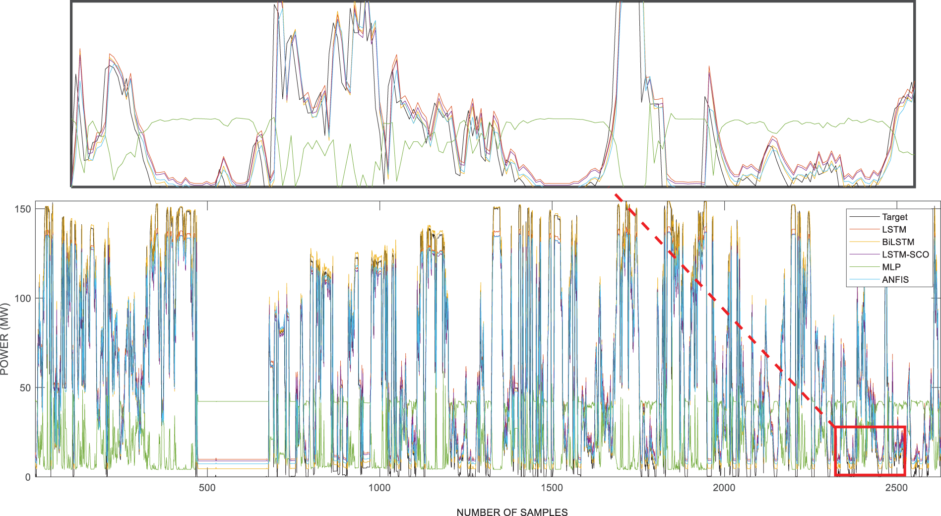
Figure 7: Results of used models for Dataset 3
By analyzing the
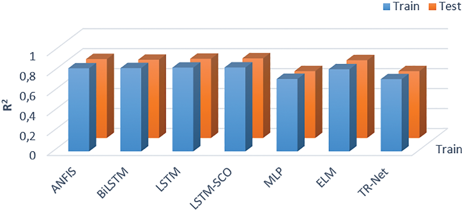
Figure 8: Results of
This study proposed a new hybrid model, LSTM-SCO, by integrating the SCO algorithm into a traditional LSTM model. The SCO algorithm determines the initial parameters of the LSTM model, improves the starting point of the model, and speeds up the optimization process, resulting in improved performance. This method introduces a novel approach for wind power forecasting with faster runtime. The success of the LSTM-SCO model was assessed using various performance metrics in the results section, demonstrating the potential of this new hybrid model in the field of wind power forecasting.
The study applied the proposed LSTM-SCO hybrid model to observed wind data from three offshore wind-energy farms and developed a highly accurate prediction model. The model outperformed benchmark models, including LSTM, BiLSTM, MLP, and ANFIS, thereby demonstrating its superior accuracy. The results showed that the LSTM-SCO hybrid model was the most successful. In the Dataset 2, the LSTM-SCO model outperformed all other models in both the training and testing phases. By integrating the SCO metaheuristic approach into the LSTM model, there was a noticeable 12.5% enhancement in terms of the MSE value for Dataset 2. Similarly, in the Dataset 1 and Dataset 3, the LSTM-SCO model was more successful in both training and testing, except for the MAE values. Consequently, the proposed hybrid LSTM-SCO model outperformed singular forecasting models, as demonstrated in this study.
In addition to improvements observed in terms of MSE and MAE, the proposed LSTM-SCO model also achieved noticeable enhancements in MARE across all datasets. For instance, in Dataset 2, the test phase MARE value of the LSTM-SCO model was 0.1447, which corresponds to a relative error reduction of 6.7% compared with the baseline LSTM model. Similarly, in Dataset 1 and Dataset 3, the LSTM-SCO model yielded lower MARE values than all other models except BiLSTM, further confirming its robustness and effectiveness in minimizing relative forecasting errors.
The results obtained in this study can contribute to the groundwork of further research. The structural description of the proposed LSTM-SCO model and the ability of the SCO algorithm to optimize the initial parameters provide insight into the development of new approaches in the domain of wind energy prediction. Future studies may aim to integrate data preprocessing algorithms into this model and make it compatible with different optimization techniques. Furthermore, evaluating the performance of the LSTM-SCO model on different datasets and time intervals is an important research area. Based on the results of the proposed hybrid model, this study contributes to the development of more effective and accurate models for different regions.
Although the proposed LSTM-SCO hybrid model demonstrated superior performance across multiple offshore wind power datasets, several challenges and limitations should be acknowledged, offering avenues for future research. While the SCO algorithm offers a lightweight and fast convergence solution compared to population-based metaheuristics, its single-solution-based strategy may limit the exploration capability in highly complex optimization landscapes. Additionally, because SCO was employed only for the initialization of the LSTM parameters, potential improvements from deeper integration during training were not explored. Another limitation stems from the use of a relatively fixed LSTM architecture across the different datasets. More adaptive architectures may yield enhanced performances. Furthermore, the model was validated for one-hour-ahead forecasting using historical offshore wind data sets. Real-world applications may involve more dynamic or noisy environments, grid constraints, or missing data, which were not addressed in the current study.
To further improve model performance and robustness, future studies may incorporate decomposition-based preprocessing techniques such as VMD, CEEMDAN, or wavelet transforms to better extract signal components. In addition, hybrid models can be extended to include ensemble or attention-based architectures to better capture temporal dependencies. The integration of LLM-based time-series forecasters presents a novel research avenue, either through intra-modal fine-tuning or cross-modal prompting, especially in scenarios with limited training data.
Acknowledgement: The authors have no acknowledgments to declare.
Funding Statement: The authors received no specific funding for this study.
Author Contributions: Conceptualization, Mehmet Balci, Emrah Dokur and Ugur Yuzgec; methodology, Mehmet Balci, Emrah Dokur and Ugur Yuzgec; software, Mehmet Balci and Ugur Yuzgec; validation, Emrah Dokur and Ugur Yuzgec; formal analysis, Ugur Yuzgec; investigation, Mehmet Balci; resources, Mehmet Balci and Emrah Dokur; data curation, Mehmet Balci and Ugur Yuzgec; writing—original draft preparation, Mehmet Balci; writing—review and editing, Emrah Dokur and Ugur Yuzgec; visualization, Mehmet Balci, Emrah Dokur and Ugur Yuzgec. All authors reviewed the results and approved the final version of the manuscript.
Availability of Data and Materials: The data that support the findings of this study are available from the authors upon reasonable request.
Ethics Approval: Not applicable.
Conflicts of Interest: The authors declare no conflicts of interest to report regarding the present study.
Abbreviations
| AGRU | Attention-based Gated Recurrent Unit |
| AI | Artificial Intelligence |
| ANN | Artificial Neural Network |
| ANFIS | Adaptive-Network-Based Fuzzy Inference System |
| ARIMA | Autoregressive Integrated Moving Average |
| ARMA | Autoregressive Moving Average |
| AVMD-ODRMKELM | Adaptive Variational Mode Decomposition and Optimized Deep Learning Mixed Kernel Extreme Learning Machine |
| BiLSTM | Bidirectional Long Short-Term Memory |
| CEEMDAN | Complete Ensemble Empirical Mode Decomposition with Adaptive Noise |
| CNN | Convolutional Neural Network |
| CSA | Crow Search Algorithm |
| ELM | Extreme Learning Machine |
| FS | Feature Selection |
| FS-BO-BILSTM | Feature Selection, Bayesian Optimization and Bidirectional Long Short-Term Memory |
| GA | Genetic Algorithm |
| GPT4TS | Generative Pre-trained Transformer for Time Series |
| GRU | Gated Recurrent Units |
| GW | Gigawatt |
| GWEC | Global Wind Energy Council |
| GWO | Grey Wolf Optimizer |
| GWO-LSTM | Grey Wolf Optimizer and Long Short-Term Memory |
| GWO-nested CEEMDAN-CNN-BiLSTM | Grey Wolf Optimizer, Complete Ensemble Empirical Mode Decomposition with Adaptive Noise, Convolutional Neural Network and Bidirectional Long Short-Term Memory |
| HBO-LSTM | Heap-Based Optimizer and Long Short-Term Memory |
| HBO | Heap-Based Optimizer |
| ICEEMDAN–LSTM–GWO | Improved Complementary Ensemble Empirical Mode Decomposition with Adaptive Noise, Long Short-Term Memory and Grey Wolf Optimizer |
| IEA | International Energy Agency |
| LCWOA-ELM | Lévy Flight Chaotic Whale Optimization Algorithm and Extreme Learning Machine |
| LCWOA | Lévy flight Chaotic Whale Optimization Algorithm |
| LLMs | Large Language Models |
| LSTM | Long Short-Term Memory |
| LSTM-GWO | Long Short-Term Memory and Grey Wolf Optimizer |
| LSTM-SCO | Long Short-Term Memory and Single Candidate Optimizer |
| MAE | Mean Absolute Error |
| MARE | Mean Absolute Relative Error |
| MLP | Multi-Layer Perceptron |
| MLP-WOA | Multi-Layer Perceptron and Whale Optimization Algorithm |
| MSE | Mean Squared Error |
| MSRE | Mean Squared Relative Error |
| QPSO | Quantum Particle Swarm Optimization Algorithm |
| R-squared (Coefficient of Determination) | |
| RNNs | Recurrent Neural Networks |
| RMSE | Root Mean Squared Error |
| RMSPE | Root Mean Squared Percentage Error |
| SARIMA | Seasonal Autoregressive Integrated Moving Average |
| SCO | Single Candidate Optimizer |
| SWD-Meta-ELM | Swarm Decomposition and Meta-Extreme Learning Machine |
| SVM | Support Vector Machine |
| TR-Net | Transformer Model |
| VMD | Variational Mode Decomposition |
| WT | Wavelet Transform |
| WT-DBN-LGBM | Wavelet Transform, Deep Belief Network and Light Gradient Boosting Machine |
| WT-DBN-RF | Wavelet Transform, Deep Belief Network and Random Forest |
| WPD-PSR-ADQPSO-MKLSSVM | Wavelet Packet Decomposition, Phase Space Reconstruction, Quantum Particle Swarm Optimization with Chaos Initialization, Gaussian Distribution Local Attraction Points and Disturbance Operator and Multi-Kernel Least Square Support Vector Machine |
| First input for Long Short-Term Memory | |
| Preceding cell state for Long Short-Term Memory | |
| Cell state for Long Short-Term Memory | |
| Forget gate for Long Short-Term Memory | |
| Input gate for Long Short-Term Memory | |
| W | Weight of the input connections for Long Short-Term Memory |
| U | Weight of the recurrent connections for Long Short-Term Memory |
| Stands for bias vector for Long Short-Term Memory | |
| Subscript iteration for Long Short-Term Memory | |
| Sigma activation function for Long Short-Term Memory | |
| Hidden state vector for Long Short-Term Memory | |
| Prior memory state for Long Short-Term Memory | |
| Output gate for Long Short-Term Memory | |
| Defines candidate solution position for Single Candidate Optimization Algorithm | |
| Indicates the dimension for Single Candidate Optimization Algorithm | |
| Represents the weight for Single Candidate Optimization Algorithm | |
| Stands for the best candidate solution for Single Candidate Optimization Algorithm | |
| Constant for Single Candidate Optimization Algorithm | |
| Current iteration for Single Candidate Optimization Algorithm | |
| Maximum iteration count for Single Candidate Optimization Algorithm | |
| Random number for Single Candidate Optimization Algorithm | |
| Upper limit for Single Candidate Optimization Algorithm | |
| Lower limit for Single Candidate Optimization Algorithm | |
| Stand for the random numbers in Single Candidate Optimization Algorithm | |
| Input-to-hidden weights for Long Short-Term Memory-Single Candidate Optimization Algorithm | |
| Hidden-to-hidden weights for Long Short-Term Memory-Single Candidate Optimization Algorithm | |
| Bias vectors for Long Short-Term Memory-Single Candidate Optimization Algorithm | |
| Actual wind power value at time | |
| Prediction made by the Long Short-Term Memory-Single Candidate Optimization Algorithm | |
| X | Parameters for Long Short-Term Memory-Single Candidate Optimization Algorithm |
| N | Number of training samples for Long Short-Term Memory-Single Candidate Optimization Algorithm |
| Selected as the initial set of parameters for Long Short-Term Memory-Single Candidate Optimization Algorithm | |
| Learning rate for Long Short-Term Memory-Single Candidate Optimization Algorithm | |
| A small constant to prevent division by zero for Long Short-Term Memory-Single Candidate Optimization Algorithm | |
| Exponential decay rates for the moment estimates in Long Short-Term Memory-Single Candidate Optimization Algorithm |
References
1. I. E. A. (IEA). World energy balances: overview world; 2020 [Internet]. [cited 2023 Sep 15]. Available from: https://www.iea.org/reports/world-energy-balances-overview/world. [Google Scholar]
2. Sun S, Du Z, Jin K, Li H, Wang S. Spatiotemporal wind power forecasting approach based on multi-factor extraction method and an indirect strategy. Appl Energy. 2023;350(2):121749. doi:10.1016/j.apenergy.2023.121749. [Google Scholar] [CrossRef]
3. Wu YK, Hong JS. A literature review of wind forecasting technology in the world. In: 2007 IEEE Lausanne Power Tech; 2007 Jul 1–5; Lausanne, Switzerland. p. 504–9. doi:10.1109/PCT.2007.4538368. [Google Scholar] [CrossRef]
4. Wang J, Qian Y, Zhang L, Wang K, Zhang H. A novel wind power forecasting system integrating time series refining, nonlinear multi-objective optimized deep learning and linear error correction. Energy Convers Manag. 2024;299:117818. doi:10.1016/j.enconman.2023.117818. [Google Scholar] [CrossRef]
5. Li N, Dong J, Liu L, Li H, Yan J. A novel EMD and causal convolutional network integrated with Transformer for ultra short-term wind power forecasting. Int J Electr Power Energy Syst. 2023;154(3):109470. doi:10.1016/j.ijepes.2023.109470. [Google Scholar] [CrossRef]
6. Dokur E, Karakuzu C, Yüzgeç U, Kurban M. Using optimal choice of parameters for meta-extreme learning machine method in wind energy application. COMPEL. 2021;40(3):390–401. doi:10.1108/COMPEL-07-2020-0246. [Google Scholar] [CrossRef]
7. Hong YY, Rioflorido CLPP, Zhang W. Hybrid deep learning and quantum-inspired neural network for day-ahead spatiotemporal wind speed forecasting. Expert Syst Appl. 2024;241(2):122645. doi:10.1016/j.eswa.2023.122645. [Google Scholar] [CrossRef]
8. Zheng J, Wang J. Short-term wind speed forecasting based on recurrent neural networks and Levy crystal structure algorithm. Energy. 2024;293:130580. doi:10.1016/j.energy.2024.130580. [Google Scholar] [CrossRef]
9. Zhang D, Hu G, Song J, Gao H, Ren H, Chen W. A novel spatio-temporal wind speed forecasting method based on the microscale meteorological model and a hybrid deep learning model. Energy. 2024;288:129823. doi:10.1016/j.energy.2023.129823. [Google Scholar] [CrossRef]
10. Balci M, Dokur E, Yuzgec U, Erdogan N. Multiple decomposition-aided long short-term memory network for enhanced short-term wind power forecasting. IET Renew Power Gener. 2024;18(3):331–47. doi:10.1049/rpg2.12919. [Google Scholar] [CrossRef]
11. Tawn R, Browell J. A review of very short-term wind and solar power forecasting. Renew Sustain Energ Rev. 2022;153(10):111758. doi:10.1016/j.rser.2021.111758. [Google Scholar] [CrossRef]
12. Hong T, Pinson P, Wang Y, Weron R, Yang D, Zareipour H. Energy forecasting: a review and outlook. IEEE Open Access J Power Energy. 2020;7:376–88. doi:10.1109/OAJPE.2020.3029979. [Google Scholar] [CrossRef]
13. Yang T, Yang Z, Li F, Wang H. A short-term wind power forecasting method based on multivariate signal decomposition and variable selection. Appl Energy. 2024;360(15):122759. doi:10.1016/j.apenergy.2024.122759. [Google Scholar] [CrossRef]
14. Chen N, Qian Z, Nabney IT, Meng X. Wind power forecasts using Gaussian processes and numerical weather prediction. IEEE Trans Power Syst. 2013;29(2):656–65. doi:10.1109/TPWRS.2013.2282366. [Google Scholar] [CrossRef]
15. Zhao J, Guo Y, Xiao X, Wang J, Chi D, Guo Z. Multi-step wind speed and power forecasts based on a WRF simulation and an optimized association method. Appl Energy. 2017;197:183–202. doi:10.1016/j.apenergy.2017.04.017. [Google Scholar] [CrossRef]
16. Jung J, Broadwater RP. Current status and future advances for wind speed and power forecasting. Renew Sustain Energ Rev. 2014;31:762–77. doi:10.1016/j.rser.2013.12.054. [Google Scholar] [CrossRef]
17. Erdem E, Shi J. ARMA based approaches for forecasting the tuple of wind speed and direction. Appl Energy. 2011;88(4):1405–14. doi:10.1016/j.apenergy.2010.10.031. [Google Scholar] [CrossRef]
18. Liu X, Lin Z, Feng Z. Short-term offshore wind speed forecast by seasonal ARIMA—a comparison against GRU and LSTM. Energy. 2021;227:120492. doi:10.1016/j.energy.2021.120492. [Google Scholar] [CrossRef]
19. Singh SN, Mohapatra A. Repeated wavelet transform based ARIMA model for very short-term wind speed forecasting. Renew Energy. 2019;136(1):758–68. doi:10.1016/j.renene.2019.01.031. [Google Scholar] [CrossRef]
20. Wang J, Niu X, Zhang L, Liu Z, Huang X. A wind speed forecasting system for the construction of a smart grid with two-stage data processing based on improved ELM and deep learning strategies. Expert Syst Appl. 2024;241(4):122487. doi:10.1016/j.eswa.2023.122487. [Google Scholar] [CrossRef]
21. Abedinia O, Ghasemi-Marzbali A, Shafiei M, Sobhani B, Gharehpetian GB, Bagheri M. A multi-level model for hybrid short term wind forecasting based on SVM, wavelet transform and feature selection. In: 2022 IEEE International Conference on Environment and Electrical Engineering and 2022 IEEE Industrial and Commercial Power Systems Europe (EEEIC/I&CPS Europe); 2022 Jun 28–Jul 1;Prague, Czech Republic. p. 1–6. doi:10.1109/EEEIC/ICPSEurope54979.2022.9854519. [Google Scholar] [CrossRef]
22. Zhang Y, Pan G, Chen B, Han J, Zhao Y, Zhang C. Short-term wind speed prediction model based on GA-ANN improved by VMD. Renew Energy. 2020;156(1):1373–88. doi:10.1016/j.renene.2019.12.047. [Google Scholar] [CrossRef]
23. Rayi VK, Mishra SP, Naik J, Dash PK. Adaptive VMD based optimized deep learning mixed kernel ELM autoencoder for single and multistep wind power forecasting. Energy. 2022;244(2):122585. doi:10.1016/j.energy.2021.122585. [Google Scholar] [CrossRef]
24. Samadianfard S, Hashemi S, Kargar K, Izadyar M, Mostafaeipour A, Mosavi A, et al. Wind speed prediction using a hybrid model of the multi-layer perceptron and whale optimization algorithm. Energy Rep. 2020;6(3):1147–59. doi:10.1016/j.egyr.2020.05.001. [Google Scholar] [CrossRef]
25. Memarzadeh G, Keynia F. A new short-term wind speed forecasting method based on fine-tuned LSTM neural network and optimal input sets. Energy Convers Manag. 2020;213:112824. doi:10.1016/j.enconman.2020.112824. [Google Scholar] [CrossRef]
26. Joseph LP, Deo RC, Prasad R, Salcedo-Sanz S, Raj N, Soar J. Near real-time wind speed forecast model with bidirectional LSTM networks. Renew Energy. 2023;204(7):39–58. doi:10.1016/j.renene.2022.12.123. [Google Scholar] [CrossRef]
27. He JJ, Yu CJ, Li YL, Xiang HY. Ultra-short term wind prediction with wavelet transform, deep belief network and ensemble learning. Energy Convers Manag. 2020;205:112418. doi:10.1016/j.enconman.2019.112418. [Google Scholar] [CrossRef]
28. Niu Z, Yu Z, Tang W, Wu Q, Reformat M. Wind power forecasting using attention-based gated recurrent unit network. Energy. 2020;196(3):117081. doi:10.1016/j.energy.2020.117081. [Google Scholar] [CrossRef]
29. Duan Z, Bian C, Yang S, Li C. Prompting large language model for multi-location multi-step zero-shot wind power forecasting. Expert Syst Appl. 2025;280(3):127436. doi:10.1016/j.eswa.2025.127436. [Google Scholar] [CrossRef]
30. Lai Z, Wu T, Fei X, Ling Q. BERT4ST: fine-tuning pre-trained large language model for wind power forecasting. Energy Convers Manag. 2024;307(8):118331. doi:10.1016/j.enconman.2024.118331. [Google Scholar] [CrossRef]
31. Ewees AA, Al-qaness MA, Abualigah L, Abd Elaziz M. HBO-LSTM: optimized long short term memory with heap-based optimizer for wind power forecasting. Energy Convers Manag. 2022;268(16):116022. doi:10.1016/j.enconman.2022.116022. [Google Scholar] [CrossRef]
32. Altan A, Karasu S, Zio E. A new hybrid model for wind speed forecasting combining long short-term memory neural network, decomposition methods and grey wolf optimizer. Appl Soft Comput. 2021;100(4):106996. doi:10.1016/j.asoc.2020.106996. [Google Scholar] [CrossRef]
33. Syama S, Ramprabhakar J, Anand R, Guerrero JM. A hybrid extreme learning machine model with lévy flight chaotic whale optimization algorithm for wind speed forecasting. Res Eng. 2023;19(1):101274. doi:10.1016/j.rineng.2023.101274. [Google Scholar] [CrossRef]
34. Dokur E, Erdogan N, Salari ME, Karakuzu C, Murphy J. Offshore wind speed short-term forecasting based on a hybrid method: swarm decomposition and meta-extreme learning machine. Energy. 2022;248:123595. doi:10.1016/j.energy.2022.123595. [Google Scholar] [CrossRef]
35. Sun S, Wang Y, Meng Y, Wang C, Zhu X. Multi-step wind speed forecasting model using a compound forecasting architecture and an improved QPSO-based synchronous optimization. Energy Rep. 2022;8:9899–918. doi:10.1016/j.egyr.2022.07.164. [Google Scholar] [CrossRef]
36. Phan QB, Nguyen TT. Enhancing wind speed forecasting accuracy using a GWO-nested CEEMDAN-CNN-BiLSTM model. ICT Express. 2024;10(3):485–90. doi:10.1016/j.icte.2023.11.009. [Google Scholar] [CrossRef]
37. Cai Z, Dai S, Ding Q, Zhang J, Xu D, Li Y. Gray wolf optimization-based wind power load mid-long term forecasting algorithm. Comput Electr Eng. 2023;109(5):108769. doi:10.1016/j.compeleceng.2023.108769. [Google Scholar] [CrossRef]
38. Shami TM, Grace D, Burr A, Mitchell PD. Single candidate optimizer: a novel optimization algorithm. Evol Intell. 2024;17(2):863–87. doi:10.1007/s12065-022-00762-7. [Google Scholar] [CrossRef]
39. Yuan X, Karbasforoushha MA, Syah RB, Khajehzadeh M, Keawsawasvong S, Nehdi ML. An effective metaheuristic approach for building energy optimization problems. Buildings. 2022;13(1):80. doi:10.3390/buildings13010080. [Google Scholar] [CrossRef]
40. Hochreiter S, Schmidhuber J. Long short-term memory. Neural Comput. 1997;9(8):1735–80. doi:10.1162/neco.1997.9.8.1735. [Google Scholar] [PubMed] [CrossRef]
41. Wang Y, Zou R, Liu F, Zhang L, Liu Q. A review of wind speed and wind power forecasting with deep neural networks. Appl Energy. 2021;304(1):117766. doi:10.1016/j.apenergy.2021.117766. [Google Scholar] [CrossRef]
Cite This Article
 Copyright © 2025 The Author(s). Published by Tech Science Press.
This work is licensed under a Creative Commons Attribution 4.0 International License , which permits unrestricted use, distribution, and reproduction in any medium, provided the original work is properly cited.
 Downloads
 Citation Tools