Comparative Analysis of Wavelet and Hilbert Transforms for Vehicle-Based Identification of Bridge Damping Ratios

1  Introduction

Bridges have played a crucial role in the advancement of civilization, particularly since the twentieth century. As construction technologies have rapidly evolved, a wide variety of bridge designs have emerged. However, these structures inevitably degrade due to the impact of natural disasters and environmental factors. This has made structural health monitoring of bridges an essential strategy for assessing their condition and predicting their future performance. Traditionally, direct measurement has been the go-to approach in civil engineering, which requires extensive sensor installation, large-scale data processing, and traffic disruptions for bridge-specific testing, etc. The above issues indicate that the direct measurement has become less practical for monitoring numerous bridges in developed countries. To address this challenge, an alternative known as the Vehicle Scanning Method (VSM) was introduced [1]. This indirect approach leverages vehicle-bridge interaction (VBI) systems to gather data, offering a more efficient and scalable solution for bridge monitoring [2].

In VSM, a test vehicle equipped with a limited number of sensors can theoretically identify the modal parameters of a bridge by simply traversing the structure. These modal parameters serve as critical indicators of a bridge’s health condition when monitored over time. Consequently, the accurate and efficient identification of these parameters has attracted significant research attention in recent years [3–5]. In the literature, much of the research has concentrated on the method development for identifying bridge frequencies [6,7]. For instance, the techniques such as the empirical mode decomposition [8] and the singular spectrum analysis with a bandpass filter [9] were adopted to enhance bridge frequency identification. However, bridge damping plays an equally vital role, as it directly influences structural safety and service life during both the design and maintenance phases [10]. It has been shown that structural damping can reflect changes in the spectral properties of a structure due to damage, which are not easily detected through natural frequencies and mode shapes [11,12]. To date, no appropriate theoretical approach has been developed for estimating structural damping during the design stage. Hence, modal damping ratios must be obtained from in-situ dynamic tests on completed or under-construction bridges to ensure compliance with design requirements.

Operational Modal Analysis (OMA) has recently gained prominence for estimating modal damping ratios especially in long-span bridges. OMA does not require artificial excitation; instead, it leverages ambient vibrations caused by natural sources such as traffic and wind loads. Among various OMA techniques [13], time domain identification methods use time-domain signals directly from structural responses for analysis [14]. He et al. introduced a method employing two-connected vehicles and singularity spectrum analysis to extract bridge frequency-related mono-components. The damping ratio was then estimated by fitting the free-decay segments of these mono-components [15]. An orthogonal and recursive variational mode decomposition in combination with the Hilbert transform (HT) was introduced to estimate the frequencies and damping ratios of bridge structures [16]. Shang et al. proposed an enhanced logarithmic decrement method, incorporating semantic segmentation of time series to isolate the free-decay segments from recorded data for modal damping estimation [17]. However, this method demands high-quality monitoring data, and its accuracy is sensitive to model training quality. More recently, Zhang et al. introduced an advanced signal processing technique called the natural excitation technique to enhance the bridge damping ratio identification by using the damped vibration of a non-moving VBI system excited by a moving vehicle [18].

López-Aragón et al. proposed a frequency-domain method that bypasses the traditional time-domain logarithmic decrement approach [19]. Their technique involves comparing the amplitude reduction of the spectrum over different segments of the same free-decay response to compute the damping ratio. Building on this concept, several VSM-based approaches have been developed. One method employed a two-axle, rigid-mass vehicle in combination with HT and several laser sensors to estimate bridge damping [20]. A simple bridge damping formula was derived on the basis of the instantaneous amplitudes of a vehicle’s front and rear contact responses by HT [21]. A two-axle, three-mass test vehicle equipped with multiple sensors was introduced for the same purpose by considering support effect, in which HT with a bandpass filter was used [22]. As the wavelet transform (WT) has good localization characteristics in time and frequency domains, it is adopted in the identification of structural modal parameters [23–25] and bridge damage detection [26,27]. Another method utilized WT with a bandpass filter, exploiting the correlation between front and rear wheelsets of a two-axle vehicle to estimate damping by using contact-point responses [28].

The damping identification frameworks were established on the basis of installing several sensors (i.e., six) on a test vehicle in Refs. [20,22]. In view of operational efficiency for VSM-based damping estimation, the present study conducts a comparative analysis using both HT and WT techniques by only two mounted sensors. Notably, the sensors are installed in the front and rear wheel locations of the test vehicle. Corresponding formulations for estimating the damping ratio using both HT and WT are derived and analyzed. The arrangement of this paper is given below: Section 2 formulates the test vehicle-bridge system. Dealing with pavement irregularity in the finite element method (FEM) is introduced in Section 3. A comparative analysis is conducted in Section 4. Section 5 presents the investigation of key factors. The concluding remarks are drawn in Section 6.

2  Formulation of Test Vehicle-Bridge System

2.1 Closed-Form Solution for Bridge

As depicted in Fig. 1, a three-mass test vehicle [29] is adopted to scan the damping ratio of a bridge. For illustration purpose, the test vehicle is assumed to move at a constant velocity v on a simply supported bridge. For the bridge, it has mass of m¯L, flexure rigidity of EI, and a damping coefficient c. For the test vehicle, it has rigid mass of mv and two unsprung mass of mw1 and mw2 as spanned by axle distance d, in which mv has vertical and pitching degrees of freedom (DOFs) qv and θv, respectively, and mw1 and mw2 have vertical DOFs qw1 and qw2, respectively. In this study, the subscripts 1 and 2 refer to physical quantities related to the front and rear wheels. For each suspension unit, it has a spring constant kvi and a damping coefficient cvi. As a general description, the centroid of the test vehicle is located with distance d1 from the front wheel such that d=d1+d2.

Figure 1: A three-mass test vehicle moving on a simply supported bridge

In the test vehicle, the two sensors (denoted by blue dots) are used to scan the bridge responses at the scanning points (SPs) (denoted by red dots) along the bridge. The identification of bridge damping ratio will be detailed in the following.

By adopting the Euler-Bernoulli beam theory, the equation of motion of a damped bridge with lateral displacement u(x,t) can be expressed as

m¯u¨(x,t)+cu˙(x,t)+EIu′′′′(x,t)=−f1δ(x−vt)−f2δ(x−v(t−dv))(1)

where δ is the Dirac delta function; the derivatives of time and position are respectively denoted by a dot and an apostrophe in this study. For the present purpose, it is assumed that the mass of the vehicle is much smaller than that of the bridge. Thus, the effects of moving mass [30], which arise from the high suspension stiffness of the VBI system and the large vehicle-to-bridge mass ratio, can be neglected, resulting in the simplified force terms on the right-hand side of Eq. (1). By assuming the direct contact between the wheels and bridge pavement, the contact forces f1 and f2 are given by

f1=(d2dmv+mw1)g,f2=(d1dmv+mw2)g(2)

where g is the gravitational acceleration.

Upon introducing the modal superposition, the vertical displacement of the bridge can be written by the modal coordinate qbn(t) and mode shape as follows:

u(x,t)=∑n=1Nqbn(t)sin⁡nπxL(3)

Substituting Eq. (3) to Eq. (1) and following the procedure given in Ref. [30] yield the modal equation:

q¨bn(t)+2ξbnωbnq˙bn(t)+ωbn2qbn(t)=−2m¯L∑k=12fksin⁡(nπvtkL)(4)

where ωbn denotes the nth bridge angular frequency as ωbn=(nπL)2EIm¯; ξbn denotes the nth bridge damping ratio as ξbn=c2ωbnm¯; tk=t−dv(k−1) for readability.

For a two-axle vehicle load acting on the bridge, the load on the right-hand side of Eq. (4) can be decomposed into three scenarios [29]: (1) f1 on the bridge for t<dv; (2) f1 and f2 on the bridge for dv≤t<Lv; (3) f2 on the bridge for Lv≤t<L+dv. For simplicity, the method of superposition [31] for two-axle loads is adopted, in which a single axle load (i.e., fk) is firstly considered in the following derivation with zero initial conditions.

The homogeneous solution of Eq. (4) is assumed to be

qbnh(t)=C1eλt(5)

where λ=−ξbnωbn±iωdn, in which ωdn=ωbn1−ξbn2 denoting the damped bridge angular frequency. Eq. (5) can be further written as

qbnh(t)=e−ξbnωbnt[Ankcos⁡(ωdnt)+Bnksin⁡(ωdnt)](6)

The particular solution of Eq. (4) is assumed to be

qbnp(t)=Cnkcos⁡nπvtL+Dnksin⁡nπvtL(7)

In Eqs. (6) and (7), Ank, Bnk, Cnk, and Dnk are the unknown coefficients to be solved. From the inhomogeneous modal equation, Cnk and Dnk can be determined first; then, Ank and Bnk can be found from the modal equation using qbn=qbnh+qbnp.

By employing the superposition, the general expression of bridge displacement is finally reached as

u(x,t)=∑n=1N∑k=12{e−ξbnωbntk[Ankcos⁡(ωdntk)+Bnksin⁡(ωdntk)]+Cnkcos⁡nπvtkL+Dnksin⁡nπvtkL}sin⁡nπxL(8)

with

Cnk=4ξbnrnfkm¯Lωbn2[(1−rn2)2+(2ξbnrn)2],Dnk=−2(1−rn2)fkm¯Lωbn2[(1−rn2)2+(2ξbnrn)2](9)

Ank=−Cnk,Bnk=1ωdn(Ankξbnωbn−nπvLDnk)(10)

in which rn=nπvωbnL. Note that Eq. (8) applies to the scenario of two wheels on the bridge.

2.2 Closed-Form Solution for Scanning Points

Referring to Fig. 1, a three-mass test vehicle is instrumented with two sensors in the front and rear locations of the vehicle body. Particularly, the SPs are the direct projections of sensor locations onto the bridge, i.e. x1 and x2. Based on the bridge displacement in Eq. (8), the displacement of a SP can be expressed as

ubj(t)=∑n=1Nqbn(t)sin⁡nπxjL(11)

where xj=v[t−dv(j−1)] for j=1,2. Then, the response of a SP can be explicitly derived as

ubj(t)=∑n=1N∑k=12{e−ξbnωbntk[Ankcos⁡(ωdntk)+Bnksin⁡(ωdntk)]+Cnkcos⁡nπvtkL+Dnksin⁡nπvtkL}×sin⁡nπv[t−dv(j−1)]L∀j=1,2(12)

Since it is known that the bridge damping helps to reduce motion of a bridge in service, the free-decay response in the above equation is extracted as the component response ubcj,n(t), as given below:

ubcj,n(t)=∑k=12Enk[e−ξbnωbntkcos⁡ωdn(tk+βn)]sin⁡nπv[t−dv(j−1)]L ∀j=1,2(13)

with

Enk=Ank2+Bnk2,βn=cos−1⁡(AnkAnk2+Bnk2)(14)

In the next section, Eq. (13) will be adopted to derive the formula of bridge damping ratio.

2.3 WT for Identifying Bridge Damping Ratio

To transform a signal Y(t) from the time domain into the time-frequency domain, the WT is adopted, which is defined by

W(a,b)=1a∫−∞∞Y(t)ψ∗(t−ba)dt(15)

in which W(a,b) is the wavelet coefficient involving a scale parameter a for stretch of the wavelet and a time parameter b for translation of the wavelet. ψ is the wavelet basis function while ψ∗ is the conjugate function of the mother wavelet ψ. The Morlet wavelet ψ and its complex conjugate ψ∗ are expressed as

ψ(t)=eiω0te−t22(16)

with the wavelet central angular frequency denoted by ω0.

In Eq. (15), the scale parameter a and the signal pseudo-frequency f have the following relation:

a=Fc×Fsf(17)

where the central frequency is defined as Fc=ω02π, which is a default value in Matlab R2023a. Fs is the sampling frequency, which is Fs=1Δt=10.001=1000 in this study.

By using the asymptotic technique [28], the WT can be written as

Wj(a,b)=1a∫−∞∞Aj(t)cos⁡[ϕ(t)]ψ∗(t−ba)dt∀j=1,2=a2Aj(b)Ψ∗[aϕ′(b)]eiϕ(b)∀j=1,2(18)

in which Aj(t)cos⁡[ϕ(t)] denotes the signal. By introducing the component response in Eqs. (13)–(18), the WT of the nth component response can be derived as

Wbcj,n(a,b)=a2En[f1e−ξbnωbnbeiωdn(b+βn)+f2e−ξbnωbn(b−dv)eiωdn(b−dv+βn)]×sin⁡nπv[b−dv(j−1)]LΨ∗(aωdn)∀j=1,2(19)

with Enk=Enfk. The above nth WT reaches a maximum value |Wbcj,n(an,b)| when an=ω0/ωdn. Then, the nth wavelet coefficients corresponding to the front and rear wheels are given by

|Wbc1,n(an,b)|=|an2En[f1e−ξbnωbnb+f2e−ξbnωbn(b−dv)]sin⁡nπvbLΨ∗(anωdn)|(20)

|Wbc2,n(an,b)|=|an2En[f1e−ξbnωbnb+f2e−ξbnωbn(b−dv)]sin⁡nπv(b−dv)LΨ∗(anωdn)|(21)

with the two wavelet coefficients derived on the basis of a three-mass test vehicle, the damping ratio of the bridge can be formulated as follows:

|Wbc2,n(an,b+dv)||Wbc1,n(an,b)|=e−ξbnωbndv(22)

where the lagging of time between the two wheels is introduced through the axial distance of the vehicle. Thus, the bridge damping ratio described by the WT is derived:

ξbn=−ln⁡[|Wbc2,n(an,b+d/v)||Wbc1,n(an,b)|]ωbndv(23)

2.4 HT for Identifying Bridge Damping Ratio

For a signal s(t), the HT of s(t) can be defined by [20,22]

h(t)=H[s(t)]=1π∫−∞∞s(τ)t−τdτ(24)

The original s(t) and the convolution of s(t) constitute an analytical signal Y(t), i.e. Y(t)=s(t)+ih(t). The instantaneous amplitue of Y(t) is

A(t)=[s(t)]2+[h(t)]2(25)

Upon applying HT to the component response ubcj,n(t) in Eq. (13), the nth instantaneous amplitude of the component response corresponding to the front and rear wheels are described by

A[ubc1,n(t)]=En[f1e−ξbnωbnt+f2e−ξbnωbn(t−dv)]sin⁡nπvtL(26)

A[ubc2,n(t)]=En[f1e−ξbnωbnt+f2e−ξbnωbn(t−dv)]sin⁡nπv(t−dv)L(27)

In a similar way to the WT, the damping ratio of the bridge can be formulated below:

A[ubc2,n(t+dv)]A[ubc1,n(t)]=e−ξbnωbndv(28)

Thus, the bridge damping ratio described by the HT is derived as

ξbn=−ln⁡[A[ubc2,n(t+d/v)]A[ubc1,n(t)]]ωbndv(29)

From Eqs. (23) and (29), it has shown that the bridge damping ratio can be estimated using the ratio of either the coefficients or the amplitudes of signals at two measurement points, regardless of the bridge boundary conditions. To further investigate this point, a continuous bridge with various span numbers will be analyzed in the parametric study. In VSM, since the vehicle-to-bridge mass ratio is extremely small in real-world conditions, it is expected that ongoing traffic will not influence the damping ratio identification, as demonstrated in previous studies [28].

3  Pavement Irregularity in Finite Element Method

FEM will be adopted in the numerical analysis. For the bridge, the Rayleigh damping is assumed. The equations of a VBI system can be referred to the previous studies [22,29]. To consider practical applications, the pavement irregularity cannot be neglected. To this end, the subtraction strategy using residual responses is introduced. As shown in Fig. 2, an additional sensor is installed in the centroid of the vehicle body so that three residual responses can be found.

Figure 2: A VBI system under pavement irregularity

The distances between the sensors and SPs are denoted by Δy1, Δyc, and Δy2. As accelerometers are commonly used in structural health monitoring, the corresponding acceleration responses of Δy1, Δyc, and Δy2 are defined as

Δy¨1(t)=q¨v(t)+d1θ¨v(t)−u¨bc1(t)−r¨1,Δy¨c(t)=q¨v(t)−u¨bcc(t)−r¨c,Δy¨2(t)=q¨v(t)−d2θ¨v(t)−u¨bc2(t)−r¨2(30)

where the pavement irregularities at x1, xc, and x2 are respectively denoted by r1=r(x1), rc=r(xc), and r2=r(x2). Then, the acceleration responses of the three SPs can be determined by

y¨1(t)=q¨v(t)+d1θ¨v(t)−Δy¨1(t),y¨c(t)=q¨v(t)−Δy¨c(t),y¨2(t)=q¨v(t)−d2θ¨v(t)−Δy¨2(t)(31)

which implies

y¨1(t)=u¨bc1(t)+r¨1,y¨c(t)=u¨bcc(t)+r¨c,y¨2(t)=u¨bc2(t)+r¨2(32)

Finally, the three residual responses can be defined as follows:

y¨r,c1(t)=y¨c(t+d1v)−y¨1(t),y¨r,2c(t)=y¨2(t+dv)−y¨c(t+d1v),y¨r,21(t)=y¨2(t+dv)−y¨1(t)(33)

The above residual responses will be incorporated in FEM to eliminate the effect of pavement irregularity.

4  Comparative Analysis

The damping ratio of a simply supported bridge will be identified by using both HT and WT to understand the accuracy achieved by each approach. The parameters of the VBI system are given in Table 1. In this example, the effect of vehicle damping is ignored. The numerical analysis is conducted using Matlab R2023a on an Intel Core i7-9700 CPU with 48 GB RAM. In FEM, the bridge is discretized by 40 beam elements, and the dynamic equation of the VBI system is solved by Newmark β method with parameters β=1/4 and γ=1/2 for unconditional stability. The time step is 0.001 s. Unless otherwise mentioned, the parameters listed in this table [22] will be adopted in the following study.

In the FEM analysis, upon finding the acceleration response of a SP, the bandpass filter is applied, in which the target frequency is set as the first damped bridge frequency fd1 with bandwidth equal to 0.1∼0.153fd1. For illustration, the frequency spectra obtained by the bridge acceleration and vehicle acceleration are shown in Figs. 3 and 4, where the consistent results of the identified fd1 and fd2 between the analytical solution and FEM are demonstrated. Based on the information of the bandpass filter, HT and WT are further introduced. Particularly, the regression techniques in Matlab called LAR (least absolute residual) and RANSAC (random sample consensus) are respectively adopted to optimize the results. In Ref. [22], it was shown that a linear function can be fitted by using LAR. For a constant bridge damping ratio, RANSAC was adopted to fit a function with zero slope [28]. In this study, both HT and WT with LAR and RANSAC are respectively investigated.

Figure 3: Spectrum obtained by bridge acceleration

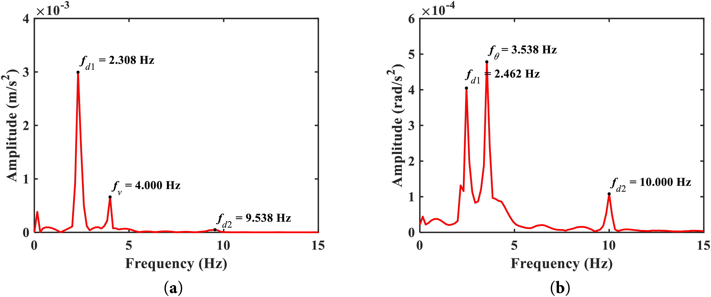
Figure 4: Spectrum by FEM: (a) vehicle vertical acceleration; (b) vehicle rotational acceleration

As shown in Fig. 5, the procedure for identifying bridge damping ratio is presented with the following description: Fig. 5a,b exhibits the SP accelerations at front wheel (denoted by HT1, WT1) and at rear wheel (denoted by HT2, WT2) by HT and WT, respectively. Then, the bridge damping ratio is estimated using the theoretical formulas in Eq. (29) for HT and Eq. (23) for WT, as presented by the blue line in Fig. 5c,d; afterward, the regression technique LAR is used to identify the bridge damping ratio ξb as denoted by the red line. Obviously, large oscillations or deviations appear at the two ends of the bridge by both HT and WT, indicating less confidence of the regression. Such a phenomenon can be attributed to the support effect. As the vehicle approaches the bridge support or enters and leaves the bridge, the dynamic response transmitted from the bridge to the vehicle diminishes, leading to reduced signal energy and a relatively increased noise level. To this end, the support effect is considered by removing the data near the two ends. For the test vehicle with axle distance d=2.5m, the data in the two regions with d=2.5m from the two ends are omitted. Finally, the identified bridge damping ratio ξb by HT and WT are shown in Fig. 5e,f, respectively. By comparing the numerical results with the theoretical value (denoted by the dashed line), the relative errors by the two signal processing techniques are summarized in Table 2. It is observed that WT has higher accuracy over HT with and without considering the support effect. By including the support effect, the relative errors can be largely reduced. Similarly, the numerical results by RANSAC are shown in Fig. 6 with relative errors listed in Table 2; improved results are obtained when the support effect is considered. Again, higher accuracy is ensured by using WT. Extraordinarily, RANSAC exhibits better fitting ability for bridge damping identification. Therefore, RANSAC will be adopted in the subsequent analysis.

Figure 5: Procedure for identifying bridge damping ratio by LAR (left column for HT; right column for WT): (a,b) SP accelerations at two wheels; (c,d) identified ξb; (e,f) identified ξb with support effect

Figure 6: Identified bridge damping ratio by RANSAC (left column for HT; right column for WT): (a,b) identified ξb; (c,d) identified ξb with support effect

5  Parametric Study

In this section, a parametric study is conducted to evaluate the derived formulas for bridge damping ratio identification. To meet practical concerns, the following key factors are included: the test vehicle’s centroid location, the influence of pavement irregularity, different bridge modal damping ratios, the number of spans in a continuous bridge, and the influence of bridge damping ratios. A systematic analysis will be provided for each factor in the following content.

5.1 Effect of Vehicular Centroid Location

Referring to Fig. 1, the centroid of a two-axle test vehicle may not be designed in the center of the vehicle body to meet certain purpose. To consider such a situation, five cases of vehicles with different centroid locations are investigated, as listed in Table 3. Upon considering the support effect, by careful inspection, the above results reveal that if the vehicular centroid locates in the half part of the vehicle (i.e. smaller d2) for vehicle passage in the positive x direction, it is beneficial to the identification of bridge damping ratio as the relative errors for both HT and WT are smaller than the cases of smaller d1.

5.2 Effect of Pavement Irregularity vs. Different Bridge Damping Ratios

The influence of pavement irregularity on the identification of bridge damping ratio is investigated by using ISO 8608 [32] to numerically generate the pavement profiles of Class A and Class B as shown in Fig. 7, in which each dataset is averaged by 20 sets of individual irregularities. To remove the adverse effect of pavement irregularity, the subtraction strategy is adopted [15,16,22]. To this end, one additional sensor is installed in the centroid of the vehicle body so that three residual responses can be defined as described in Section 3. In the following, different bridge damping ratios of 0.01 and 0.02 are further examined for each class of pavement irregularity.

Figure 7: Pavement irregularity

For illustration, the numerical results under Class A pavement irregularity are presented in Fig. 8, in which the support effect is considered by omitting the data near the two bridge ends. The corresponding results are summarized in Table 4, including Class B results. By comparison, severer irregularity has larger relative error regardless of the damping ratio value. A higher damping ratio value also leads to larger relative error. Generally speaking, WT shows better accuracy in terms of bridge damping ratio identification with the aid of its composition as given in Eq. (17).

Figure 8: Identified bridge damping ratio (left column by HT; right column by WT) considering support effect: (a,b) ξb=0.01; (c,d) ξb=0.02

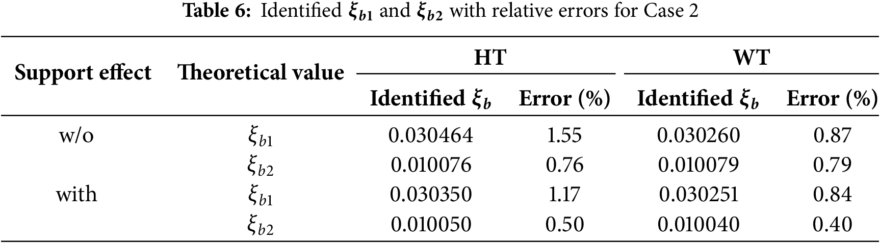
5.3 Effect of Different Bridge Modal Damping Ratios

To consider bridges of different modal damping ratios, the following two cases are designed: (1) ξb1=0.01 and ξb2=0.02; (2) ξb1=0.03 and ξb2=0.01. To retrieve two bridge modal damping ratios, the bandpass filter needs to be centered around the damped bridge frequencies fd1 and fd2 individually to target one mode at a time so that the bridge damping ratio can be identified. It is noted that fd1 and fd2 can be found from the spectrum of a test vehicle as can be referred to Section 4.

In Case 1, the bandwidth of the bandpass filter for the first mode is set to be 0.123fd1 while the bandwidth of the bandpass filter for the second mode is set as 0.139fd2. The numerical results for the first two modal damping ratios ξb1 and ξb2 are presented in Figs. 9 and 10, respectively. For clarity, the full-field results are provided to highlight the improvement in the results obtained by considering the support effect. Obviously, the relative errors have been largely reduced for both modes and signal processing techniques, with extraordinary improvement in the identification of the second bridge damping ratio, as listed in Table 5. In Case 2, the bandwidth of the bandpass filters corresponding to the target frequencies fd1 and fd2 are set as 0.148fd1 and 0.144fd2, respectively. The identified results are summarized in Table 6. Again, it is demonstrated that the procedure can be applied to identify different modal damping ratios with satisfactory results and small relative errors for both signal processing techniques. Besides, WT shows higher accuracy than HT in this regard.

Figure 9: Identified bridge damping ratio ξb1 (left column w/o support effect; right column with support effect): (a,b) by HT; (c,d) by WT

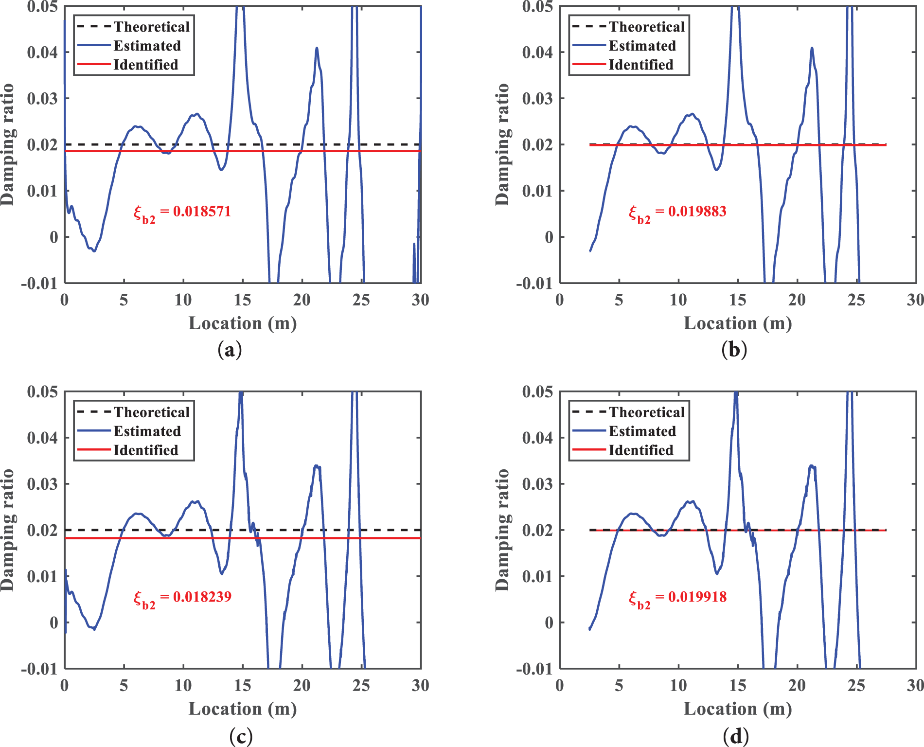
Figure 10: Identified bridge damping ratio ξb2 (left column w/o support effect; right column with support effect): (a,b) by HT; (c,d) by WT

5.4 Effect of Bridge Span Number vs. Different Bridge Damping Ratios

As most bridges are constructed as continuous bridges with several spans, the effect of span number or internal support effect is investigated in this example, in which hinged supports with span length of 15 m are assumed. In the following, four bridges of a single-span, two-span, three-span, and four-span are considered. Additionally, different bridge damping ratios of 0.01, 0.02, and 0.03 are further compared in each continuous bridge. Since WT has shown its superiority over HT in the identification of bridge damping ratio, only WT is adopted. To enhance the identification accuracy, the effect of internal support is removed via omitting the data in a support region (i.e. xi±2.5d for an internal support with a coordinate xi) [22].

For a single-span bridge, the identified bridge damping ratios for various theoretical bridge damping ratios are listed in Table 7, from which it is observed that the relative error generally increases with respect to the increase in the theoretical value of ξb while the desired accuracy is reached. For bridges of multiple spans, the identified bridge damping ratios for various theoretical bridge damping ratios are estimated by using the data collected from some of the spans or all spans to find the optimal results. For instance, in a two-span continuous bridge, the identified ξb are computed by the data from the 1st span, 2nd span, or the two spans, as compared in Table 8; by examination, using the data collected from the two spans gives the best estimation of bridge damping ratio. For a three-span continuous bridge, there are five possible combinations of the data to be used, as listed in the second column of Table 9; a careful examination reveals that using the data collected from the first two spans yields the best result of bridge damping ratio. For a four-span continuous bridge, there are seven possible combinations of the data to be used, as listed in the second column of Table 10; once again, it is found that using the data collected from the first two spans leads to the best estimation of bridge damping ratio. The above results are visualized in Fig. 11 for clarity.

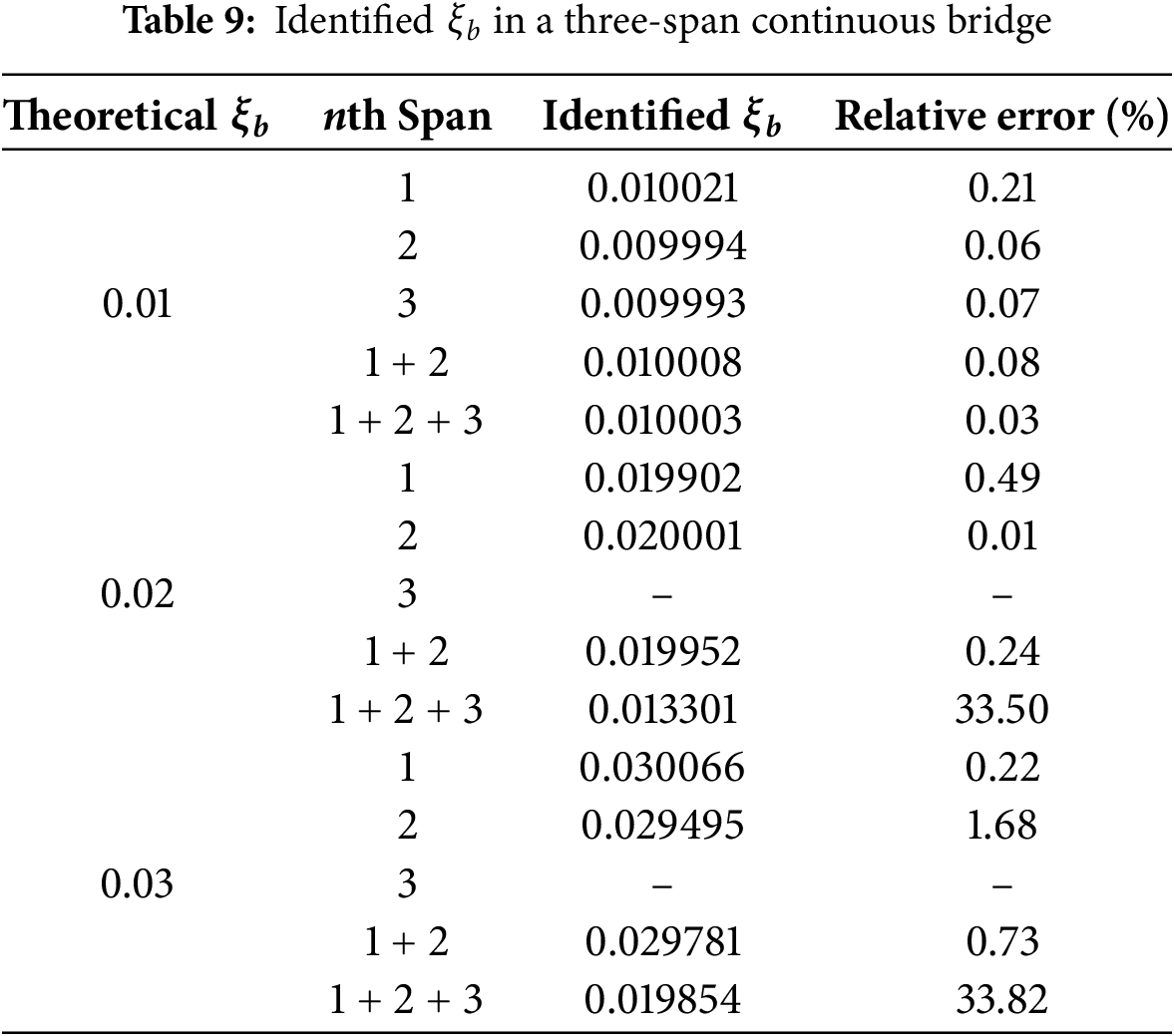
Figure 11: Identified ξb: (a) single-span bridge; (b) two-span bridge; (c) three-span bridge; (d) four-span bridge

For a damped bridge, if a test vehicle travels a longer distance on it, the recorded response may gradually be damped out during the later part of the trip. Additionally, noise arises in the signal when the vehicle approaches the supports. These factors jointly result in less accurate damping ratio identification when using data from the entire spans, e.g. very large relative errors in Tables 9 and 10. To be brief, for a multi-span bridge, the above investigation indicates that using the data collected from the first two spans gives the most satisfactory result in the identification of bridge damping ratio. Furthermore, a larger bridge damping ratio has larger identification error.

5.5 Effect of Measurement Noise

In the on-site measurement, the error of measurement can be attributed to the environmental noise or operational process. To account for such measurement noise, three different noise levels are studied through a Gaussian white noise with zero mean and unit standard deviation [22]: 1%, 3%, and 10%. By considering the support effect, the results are summarized in Table 11 and depicted in Fig. 12, in which the relative error increases with higher noise levels. Again, WT demonstrates better ability than HT in identifying bridge damping ratios.

Figure 12: Identified ξb under different noise levels (left column by HT; right column by WT): (a,b) 1%; (c,d) 3%; (e,f) 10%

6  Conclusions

Since the bridge damping ratio serves as a damage-sensitive index, advancing VSM in bridge health monitoring by estimating the damping ratio provides a fundamental basis for monitoring bridge conditions, in addition to frequency identification. In this study, the bridge damping ratio identification is effectively improved by using a two-axle three-mass test vehicle via two wheel responses, from which two sensors are shown to be adequate for estimating bridge damping ratio with desired accuracy upon considering the support effect.

Based on the numerical investigation, the following concluding remarks can be further drawn: (1) The comparative analysis of HT and WT has shown the superiority of WT over HT in the bridge damping identification. (2) According to the vehicle moving direction, it is beneficial to design a test vehicle with centroid in the half part of the vehicle body for bridge damping identification. (3) The residual response is introduced to remove the effect of pavement irregularity, while an additional sensor is required to provide information when using the derived damping ratio formulas. (4) The procedure and formulas have been demonstrated to be effective even for bridges with different modal damping ratios. (5) The numerical investigation has shown that using the responses of the first two spans of a bridge has potential for retrieving the damping ratio of a multi-span bridge.

In future studies, adopting other effective signal processing techniques could be a viable option, as the bandwidth of the bandpass filter used in this study is not clearly defined. The bandwidth size affects the precision of signal filtering, which in turn influences the accuracy of the bridge damping ratio identification.

Acknowledgement: The full support from National Science and Technology Council (NSTC) of Taiwan is acknowledged.

Funding Statement: The support is under Grant No. MOST 111-2628-E-A49-009-MY3 by NSTC, Taiwan.

Author Contributions: The authors confirm contribution to the paper as follows: conceptualization, Judy P. Yang; methodology, Judy P. Yang, Yuan-Jun Zhang; software, Yuan-Jun Zhang; formal analysis, Yuan-Jun Zhang; writing—original draft preparation, Judy P. Yang; writing—review and editing, Judy P. Yang; supervision, Judy P. Yang; funding acquisition, Judy P. Yang. All authors reviewed the results and approved the final version of the manuscript.

Availability of Data and Materials: All data generated or analyzed in this study are included in this article.

Ethics Approval: Not applicable.

Conflicts of Interest: The authors declare no conflicts of interest to report regarding this study.

References

1. Yang DS, Wang CM. Bridge damage detection using reconstructed mode shape by improved vehicle scanning method. Eng Struct. 2022;263(3–5):114373. doi:10.1016/j.engstruct.2022.114373. [Google Scholar] [CrossRef]

2. Wang ZL, Yang JP, Shi K, Xu H, Qiu FQ, Yang YB. Recent advances in researches on vehicle scanning method for bridges. Int J Str Stab Dyn. 2022;22(15):2230005. doi:10.1142/s0219455422300051. [Google Scholar] [CrossRef]

3. Tan C, Uddin N, OBrien EJ, McGetrick PJ, Kim CW. Extraction of bridge modal parameters using passing vehicle response. J Bridge Eng. 2019;24(9):04019087. doi:10.1061/(asce)be.1943-5592.0001477. [Google Scholar] [CrossRef]

4. Yang DS, Wang CM. Modal properties identification of damped bridge using improved vehicle scanning method. Eng Struct. 2022;256(2):114060. doi:10.1016/j.engstruct.2022.114060. [Google Scholar] [CrossRef]

5. Yang D, Yuan Y, Zhang J, Au FTK. Indirect bridge modal identification enhanced by iterative vehicle response demodulation. Mech Syst Signal Process. 2025;223(3–5):111831. doi:10.1016/j.ymssp.2024.111831. [Google Scholar] [CrossRef]

6. Yang YB, Zhang B, Qian Y, Wu Y. Contact-point response for modal identification of bridges by a moving test vehicle. Int J Str Stab Dyn. 2018;18(5):1850073. doi:10.1142/s0219455418500736. [Google Scholar] [CrossRef]

7. Zhang T, Xiong Z, Zhu J, Zheng K, Wu M, Li Y. Extracting bridge frequencies from the dynamic responses of moving and non-moving vehicles. J Sound Vib. 2023;564(5):117865. doi:10.1016/j.jsv.2023.117865. [Google Scholar] [CrossRef]

8. Yang YB, Chang KC. Extraction of bridge frequencies from the dynamic response of a passing vehicle enhanced by the EMD technique. J Sound Vib. 2009;322(4–5):718–39. doi:10.1016/j.jsv.2008.11.028. [Google Scholar] [CrossRef]

9. Yang YB, Chang KC, Li YC. Filtering techniques for extracting bridge frequencies from a test vehicle moving over the bridge. Eng Struct. 2013;48(12):353–62. doi:10.1016/j.engstruct.2012.09.025. [Google Scholar] [CrossRef]

10. Sadeghi-Movahhed A, De Domenico D, Mashayekhi M, Majdi A. Optimal damping of isolated tall buildings accounting for structural and nonstructural damage. J Build Eng. 2025;105(12):112497. doi:10.1016/j.jobe.2025.112497. [Google Scholar] [CrossRef]

11. Kawiecki G. Modal damping measurement for damage detection. Smart Mater Struct. 2001;10(3):466–71. doi:10.1088/0964-1726/10/3/307. [Google Scholar] [CrossRef]

12. Curadelli RO, Riera JD, Ambrosini D, Amani MG. Damage detection by means of structural damping identification. Eng Struct. 2008;30(12):3497–504. doi:10.1016/j.engstruct.2008.05.024. [Google Scholar] [CrossRef]

13. Zahid FB, Ong ZC, Khoo SY. A review of operational modal analysis techniques for in-service modal identification. J Braz Soc Mech Sci Eng. 2020;42(8):398. doi:10.1007/s40430-020-02470-8. [Google Scholar] [CrossRef]

14. Qu C, Tu G, Gao F, Sun L, Pan S, Chen D. Review of bridge structure damping model and identification method. Sustainability. 2024;16(21):9410. doi:10.3390/su16219410. [Google Scholar] [CrossRef]

15. He Y, Yang JP, Chen J. Estimating bridge modal parameters from residual response of two-connected vehicles. J Vib Eng Technol. 2023;11(7):2969–83. doi:10.1007/s42417-022-00724-4. [Google Scholar] [CrossRef]

16. Shang XQ, Huang TL, Chen HP, Ren WX, Lou ML. Recursive variational mode decomposition enhanced by orthogonalization algorithm for accurate structural modal identification. Mech Syst Signal Process. 2023;197(4–5):110358. doi:10.1016/j.ymssp.2023.110358. [Google Scholar] [CrossRef]

17. Shang Z, Xia Y, Chen L, Sun L. Damping ratio identification using attenuation responses extracted by time series semantic segmentation. Mech Syst Signal Process. 2022;180(5):109287. doi:10.1016/j.ymssp.2022.109287. [Google Scholar] [CrossRef]

18. Zhang T, Xiong Z, Zhu J, Cheng W, Wu M, Bo H, et al. Extracting bridge frequencies and damping ratios using damped vibrations of a non-moving vehicle. Mech Syst Signal Process. 2025;236:112968. doi:10.1016/j.ymssp.2025.112968. [Google Scholar] [CrossRef]

19. López-Aragón JA, Puchol V, Astiz MA. Influence of the modal damping ratio calculation method in the analysis of dynamic events obtained in structural health monitoring of bridges. J Civ Struct Health Monit. 2024;14(5):1191–213. doi:10.1007/s13349-023-00760-y. [Google Scholar] [CrossRef]

20. Yang YB, Zhang B, Chen Y, Qian Y, Wu Y. Bridge damping identification by vehicle scanning method. Eng Struct. 2019;183:637–45. doi:10.1016/j.engstruct.2019.01.041. [Google Scholar] [CrossRef]

21. Yang YB, Yang M, Liu DH, Liu YH, Xu H. Bridge damping formula based on instantaneous amplitudes of vehicle’s front and rear contact responses by Hilbert transform. Int J Str Stab Dyn. 2024;24(15):2471006. doi:10.1142/s0219455424710068. [Google Scholar] [CrossRef]

22. Yang JP, Wu CY, He Y, Zhang YJ. Framework for identifying bridge damping considering support effect using instrumented three-mass vehicle. J Vib Eng Technol. 2025;13(1):108. doi:10.1007/s42417-024-01596-6. [Google Scholar] [CrossRef]

23. Tan C, Elhattab A, Uddin N. “Drive-by’’ bridge frequency-based monitoring utilizing wavelet transform. J Civ Struct Health Monit. 2017;7(5):615–25. doi:10.1007/s13349-017-0246-3. [Google Scholar] [CrossRef]

24. Zhang M, Huang X, Li Y, Sun H, Zhang J, Huang B. Improved continuous wavelet transform for modal parameter identification of long-span bridges. Shock Vib. 2020;2020(1):4360184. doi:10.1155/2020/4360184. [Google Scholar] [CrossRef]

25. Jian X, Xia Y, Sun L. An indirect method for bridge mode shapes identification based on wavelet analysis. Struct Control Health Monit. 2020;27(12):e2630. doi:10.1002/stc.2630. [Google Scholar] [CrossRef]

26. Zhan Y, Au FTK, Zhang J. Bridge identification and damage detection using contact point response difference of moving vehicle. Struct Control Health Monit. 2021;28(12):e2837. doi:10.1002/stc.2837. [Google Scholar] [CrossRef]

27. Demirlioglu K, Erduran E. Drive-by bridge damage detection using continuous wavelet transform. Appl Sci. 2024;14(7):2969. doi:10.3390/app14072969. [Google Scholar] [CrossRef]

28. Xu H, Liu YH, Chen J, Yang DS, Yang YB. Novel formula for determining bridge damping ratio from two wheels of a scanning vehicle by wavelet transform. Mech Syst Signal Process. 2024;208(1):111026. doi:10.1016/j.ymssp.2023.111026. [Google Scholar] [CrossRef]

29. Yang JP, Sun JY. Pitching effect of a three-mass vehicle model for analyzing vehicle-bridge interaction. Eng Struct. 2020;224(4):111248. doi:10.1016/j.engstruct.2020.111248. [Google Scholar] [CrossRef]

30. Yang YB, Yau JD, Wu YS. Vehicle-bridge interaction dynamics with applications to high-speed railways. Singapore: World Scientific Publishing; 2004. [Google Scholar]

31. Biggs JM. Introduction to structural dynamics. New York, NY, USA: McGraw-Hill; 1964. [Google Scholar]

32. ISO 8608:1995. Mechanical vibration-road surface profiles-reporting of measured data. Geneva, Switzerland: International Organization for Standardization; 1995. [Google Scholar]