High-Fidelity Machine Learning Framework for Fracture Energy Prediction in Fiber-Reinforced Concrete

1  Introduction

Fracture energy describes how much energy a material can absorb after a crack has already formed, making it especially important when one wants to know how tough concrete is [1–5]. Although it still pays much attention to compressive strength, that one number often misses the full story about how concrete behaves under real-world stresses such as impacts, blasts, or powerful earthquakes. When steel or polymer fibers are mixed in, those small strands pull the broken pieces together, providing the material with an extra reserve of ductility and crack control that engineers can rely on in slender beams, slabs, or precast panels [6,7]. Understanding fracture energy as a phenomenon can be crucial in designing concrete structures that are durable and resilient. Cracking-resistant structures for bridges, pavements, tunnels, and even earthquake-resilient buildings all require durable concrete.

The three-point bending test on notched beams has become the go-to procedure for measuring fracture energy in concrete [8,9]. During the test, a notched concrete beam (typically 100 mm × 100 mm × 500 mm) is placed on two supports and loaded from above until it fails, with the crack mouth opening displacement recorded throughout. Researchers can determine the total work spent and then divide it by the area of the new crack surfaces to calculate the fracture energy. This is achieved by tracing the load vs. crack mouth opening displacement (CMOD) curve and subtracting the energy lost due to the bea’s weight. Because the setup also reveals what happens after the peak load (such as crack tip opening, fiber bridging, and pullout), the procedure provides a thorough picture of FRC toughness.

Although the three-point bending tests are precise, several limitations make them less suitable for wide-scale or general evaluations. First, the procedure demands many hours and careful steps, from cutting notches and controlling cure conditions to mounting instruments and processing data [10]. Second, testers need extra gear (such as clip gauges, LVDTs, or crack-mouth gauges) whose availability can dictate timelines and budgets. The setup is also susceptible to small changes in span-depth ratio, loading speed, or notch shape; those variables alone can cause significant differences in results from one lab to another. Due to the expense and complexity, researchers typically run only a few specimens, and tests are often limited to fixed parameters (commonly 28 days of curing, one fiber type, or a single dosage), making it difficult for findings to be easily translated to different mixes or service conditions. Variability from inconsistent fiber orientation, trapped air, operator mistakes, and other sources spoils reproducibility, making it risky to use fracture energy as a reliable comparison unless many samples are averaged together. Recent studies have leaned on data-driven methods to get around these limitations, especially machine learning, as a strong way to forecast fracture energy in FRC without the need for countless lab tests [11–13]. Rather than starting with fixed equations such as traditional empirical or semi-empirical models, machine learning looks at past measurements and picks up on the tricky, non-linear links among factors such as fiber type, fiber volume fraction, water-to-cement ratio, aggregate size, curing time, and loading rate. Within this framework, supervised regression models such as decision tree (DT), Gaussian process regression (GPR), support vector regression (SVR), artificial neural networks (ANNs), k-nearest neighbours (KNNs), random forest regression (RFR), and extreme gradient boosting regression (XGBoost) have become staples in concrete research [14–18]. For example, Khan et al. [19] paired RFR and XGBoost to forecast the compressive strength of steel-FRC, using SHAP to rank mix design factors and finding cement content ranked highest. Zhang et al. [20] explored similarly tree-based models for manufactured-sand concrete, with gradient-boosted trees delivering the best predictive scores. Wei et al. [15] trained a back-propagation neural network to estimate carbonation depth in mineral-admixed concrete, showing clearer gains over standard formulae while naming fly ash content and exposure time as key drivers. Kang et al. [17] ran eleven machine-learning algorithms against data for steel-fiber specimens, unveiling tree and boosting variants as the most reliable and spotlighting water-to-cement ratio plus silica fume as crucial inputs. Chen [16] constructed a hybrid system that fuses fuzzy logic, neural networks, and support vector machines to sharpen structural parameter estimation and damage detection in concrete beams. Tran et al. [18] examined both sole and combined models, including gradient boosting-particle swarm optimization (GB-PSO), XGBoost-PSO, and SVR-PSO to predict recycled aggregate concrete strength, with cement share emerging strongest in feature importance and partial dependence tests. GB-PSO showed the highest prediction accuracy in comparison to other models. Finally, Tarawneh et al. [21] developed a combined ANN and genetic programming model that forecasts prestress losses in girders more accurately than current design codes and shows that girder height and prestressing area are critical factors. Together, these works highlight the ability of machine learning to transform how engineers predict concrete behavior for diverse mixes, types, and structural applications.

Recent strides in machine learning and artificial intelligence are making it easier to forecast concrete fracture energy. This progress is already beating older, purely experimental and empirical methods. Nikbin et al. [11] trained an ANN on data from 246 fracture tests and used variables such as compressive strength and water-to-cement ratio to get accurate energy estimates, outperforming classic regression techniques. Xiao et al. [22] compared ridge regression, classification and regression tree (CART), and gradient-boosting regression trees (GBRT) tuned through PSO to predict the fracture energy of concrete beams on the basis of 736 data points. Their findings showed that the GBRT-PSO was the most precise model. Tran et al. [23] focused on strain-hardening fiber-reinforced composites, showed that matrix strength and fiber type shape fracture energy, and confirmed that machine learning can be a useful predictive tool for fracture energy prediction. Kumar et al. [24] utilized 87 experimental data points to evaluate the performance of four models, including XGBoost, RF, a convolutional neural network (CNN), and KNN, on high-strength and ultra-high-strength concrete, and reported that XGBoost achieved an R2 value above 0.97. Albaijan et al. [13] tested twelve classic and modern machine learning models against 500 data samples. Among these, the SVR and long short-term memory (LSTM) models proved to be the most reliable, achieving R2 values of 0.9897 and 0.9804, respectively. They also developed a user-friendly software incorporating the implemented models. On the basis of 246 data points provided in the Nikbin et al.’s [11] research, Wang et al. [25] introduced a deep learning model coupled with SHAP to interpret the influence of input variables on fracture energy, surpassing empirical formulas and improving model transparency. Kewalramani et al. [26] proposed advanced machine learning models, including AdaGrad gated recurrent unit (AdaG-GRU), adaptive response surface method with KNN (ARSM-KNN), Chi-square automatic interaction detection-decision tree (CHAID-DT), automatic linear regression with boosting overfitting criteria (ALR-OPC), and a stacking approach to predict the initial fracture energy of concrete (IFEC). A dataset of 500 samples from three-point bending tests was used for training and validation. The stacking ensemble and AdaG-GRU models achieved outstanding predictive performance (R2 = 0.98 and 0.95).

Machine-learning tools have made significant strides in predicting fracture energy in concrete; however, many of these algorithms still struggle when faced with mixes they have never encountered before. The mix in the present work includes distinct ingredients, fibre typologies, and curing methods that fall outside the scope of the data previously fed into these algorithms. As a result, existing predictors fail to provide credible estimates for the materials’ performance under crack opening and loading. That shortcoming is a clear signal that the research community must begin curating smaller, focused databases for newer concrete classes such as ultra-high-performance concrete (UHPC), strain-hardening fibre-reinforced composites, and recycled-aggregate mixes. Gathering that data will require stepwise experiments in which every variation in ingredients, placement temperature, and test age is logged in detail. Once enough richly annotated records are in hand, engineers can build deeper networks that not only beat headline accuracy benchmarks but also capture the physical pathways that govern cracking. Models such as these will enhance practicing designers’ confidence and provide codes with a firmer foundation because they relate fracture risk to a larger pool of real-world concretes. The present study aims to create and assemble a high-quality, large-scale dataset comprising 500 systematically obtained data points, enabling more accurate and precise machine learning-based fracture energy prediction algorithms.

This study aims to develop a robust and adaptable tool for forecasting fracture energy in FRC by integrating comprehensive laboratory tests with advanced machine learning methods. A central goal is to collect an unusually large, high-quality dataset that includes 500 data points. The additional samples encompass a diverse array of fiber types (including steel, glass, carbon, polypropylene, and basalt) with fiber lengths ranging from 6 to 49 mm and volume fractions between 0.51% and 2.5%. This extensive variation ensures that the database captures a wide spectrum of material behaviors and fracture responses. This rich coverage lets authors disentangle the effect of each variable and move beyond earlier studies, which often focused on only one or two fiber types and fixed combinations. The study also examines how fracture energy shifts at loading rates ranging from 0.1 kN/s to nearly 2 kN/s and charts crack growth as specimens cure for 7, 14, 28, and even 90 days, whereas much of the published work focuses on 28-day specimens kept under stable conditions. The study sheds new light on FRC’s long-range behavior and helps designers predict how structures will hold up as they age or dry by broadening the time and speed windows. A key objective of the study is to compare the predictive accuracy of several popular machine learning techniques (KNN, SVR, GPR, XGBR, ANN, and RFR) for fracture energy prediction. The work highlights which ones truly capture the nonlinear relationships between mix design variables and energy release by running all these algorithms side-by-side. Taken together, the large and varied experiments, the broad model comparison, deliberate changes in fiber and curing parameters, and long monitoring times, the work provides a unified and novel research contribution. The whole process of this study is shown in Fig. 1.

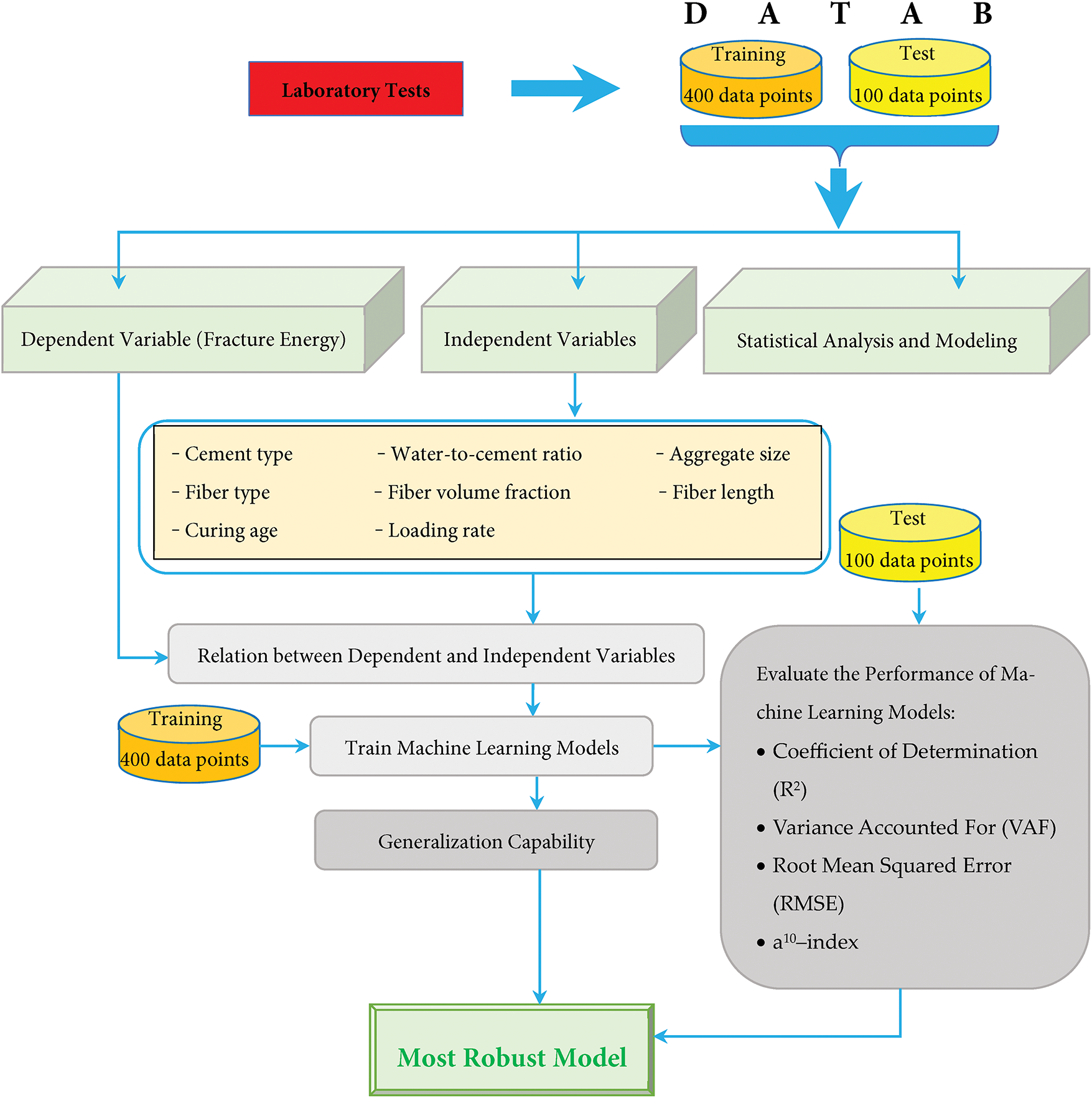
Figure 1: The whole process of this study

2  Theoretical Fundamentals of Machine Learning Algorithms

The choice of KNN, GPR, ANN, SVR, RFR, and XGBR algorithms comes from their ability to tackle the complex, nonlinear, and often high-dimensional patterns that define fracture energy in FRC. The study aims to capture every nuance in the experimental data and produce reliable predictions for engineering use by bringing together models with very different strengths. Thanks to their layered structure, ANNs quickly learn complicated, curved trends, making them a go-to tool when many variables interact and influence FRC performance at the same time. SVR, on the other hand, works really well with small to moderate sample sizes and tends to produce reliable predictions even when observations are noisy or missing. RFR and XGBR address the overfitting problem that often plagues fracture-energy forecasts by averaging multiple trees or gradually correcting errors, which typically yields steadier and more accurate results. XGBR further tightens the model through built-in regularization and smart tree pruning, meeting growing demands for explainable artificial intelligence, as engineers can now trace how certain features influence the prediction. GPR adds a layer of probabilistic thinking, providing not just a single output value but also a confidence band—a priceless feature in fracture mechanics, where consideration of data scatter and physical scatter is the rule. Lastly, the KNN method stays simple yet effective, relying on local data clusters to predict fracture energy when subtle changes in the mixture are what matter most. The researchers gain a well-rounded understanding of what prediction tools can really do for this task by weaving together everything from old-school memory methods and solid probabilistic techniques to cutting-edge ensembles and deep nets. Running all these models side by side lets them see which one consistently shines when faced with different FRC mixes and curing schedules. The goal, of course, is to build a model that scores high in accuracy yet remains easy to explain and robust when the materials or test settings change, making it genuinely useful for engineers who design with structural concrete every day. The following subsections will discuss the basic principles of each of these algorithms.

2.1 ANN

Artificial neurons draw inspiration from real nerve cells, the building blocks of biological neural networks (BNNs), which are found throughout the brain and control bodily functions. Inside a typical human nerve network, billions of these cells are found, each slightly different in shape and function. Every single neuron has four major parts (dendrites, axon, soma, and synapse), and even a simple diagram, such as the one in Fig. 2a, shows how they fit together. Modern ANNs borrow that plan, but the borrowing is casual and sometimes more poetic than scientific. Following a decades-old idea from McCulloch and Pitts [27], the first textbook picture of an ANN treats its basic building block, the artificial neuron, as a math gadget rather than a living cell. When the big homework problem needs solving, huge numbers of these math gadgets spring to life at once, crunching numbers in parallel. Each artificial neuron receives a set of inputs, labeled x, which it sums to obtain a raw output y before passing the result down the virtual circuitry. Fig. 2b indicates that the sum is sliced into smaller bits, each bit brushed with a weight w, before a non-linear twist called the activation function or transfer function f decides if the signal will really move on. An artificial neuron uses a simple mathematical formula to show how an activation function works, whether that function is a step, a sigmoid, or something else, as written in Eq. (1) [28].

yj=f(∑i=0nwijxi)(1)

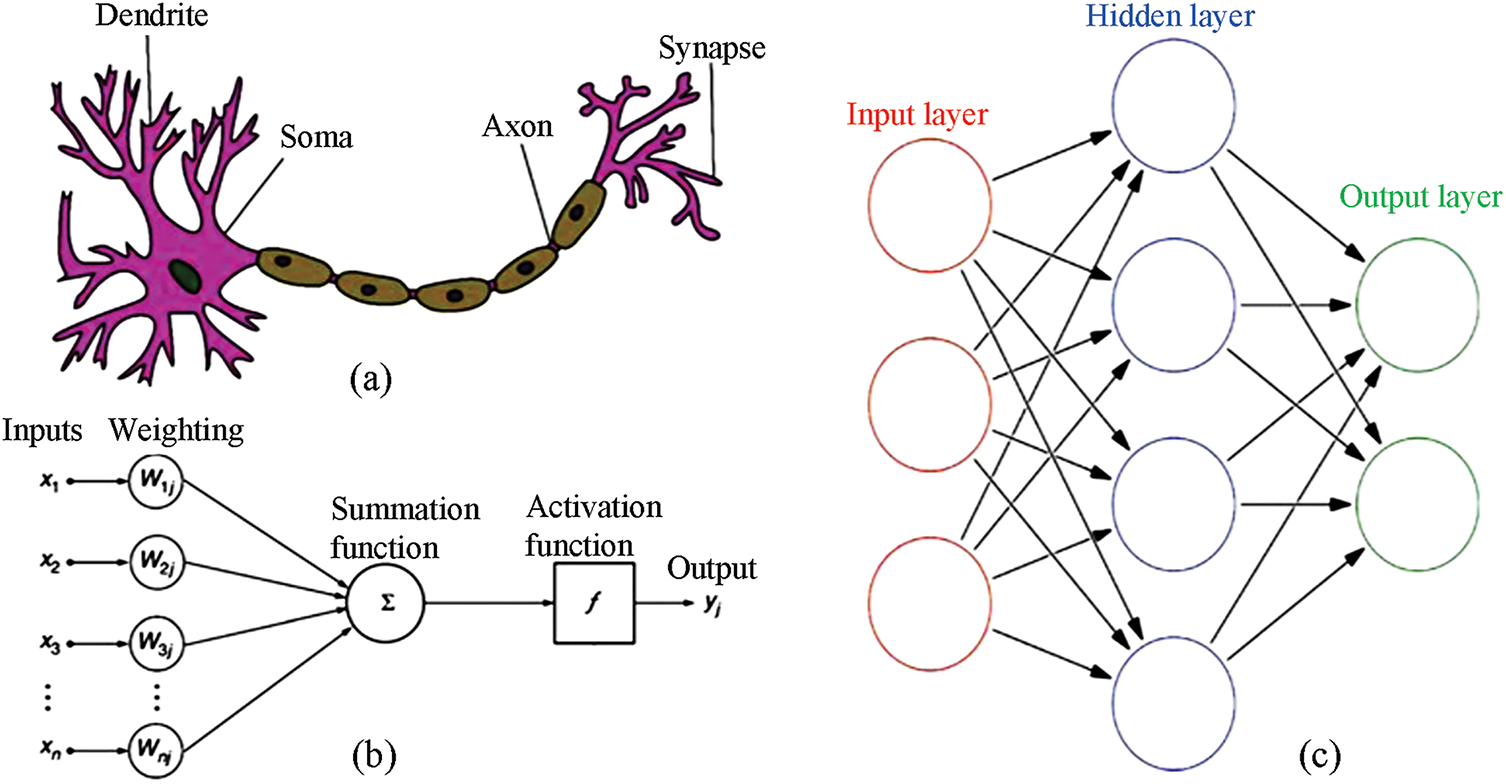
Figure 2: Working principle of ANNs. (a) A schematic drawing of biological neurons; (b) A schematic drawing of artificial neurons; (c) The structure of feed-forward ANNs [28]

In a simplified way, an artificial neuron mimics a real one by treating the axon and dendrite arrangement as the spots where incoming signals add up and where the fire-alarm-like threshold sits, the soma. The adjustable connection weights function like synapses, storing a memory of how strong each incoming signal has been. Even though these artificial cells can be strung together in almost any fashion, every lineup creates a separate network design and set of rules. Fig. 2c shows a classic feed-forward layout, the most basic shape, where data only moves ahead and never loops back. Its first layer gathers the input neurons, each of which translates raw numbers into tiny signals. Those signals then pass through one or more hidden layers, doing little bits of math along the way, before finally lighting up the output layer with the answer. Unlike the usual von-Neumann machine that follows a fixed script, the ANN updates itself over time, learning piece by piece by chewing through many examples. The most common method for training it is called supervised learning, where the system compares its guess to the true answer and then spreads any mistakes backward to tweak the connection strengths [28].

2.2 SVR

SVR is a popular method within the larger support vector machine family, and it is specifically designed for handling regression tasks [29]. At its heart, the approach measures how far the nearest training points sit from a central red line, or hyperplane, to shape the model. The actual formula that describes this prediction process can be seen in Eq. (2) [30].

y^=w⋅x+b(2)

where y^, w, and b are the predicted value, weight, and bias, respectively.

In non-linear regression tasks, SVR employs kernel functions to lift the data into a higher dimension where a linear boundary can be found. Once in this expanded space, SVR searches for the best hyperplane that hugs the sample points as closely as possible. Because of this dimensional shift, the formula for the predicted output looks different, as shown in Eq. (3) [29].

y^=w⋅∅(x)+b(3)

where ∅(x) simply represents the chosen kernel mapping for input x. Polynomial kernels and radial-basis-function kernels are among the most widely used. The impact of applying such kernels within SVR is visually summarized in Fig. 3b [30].

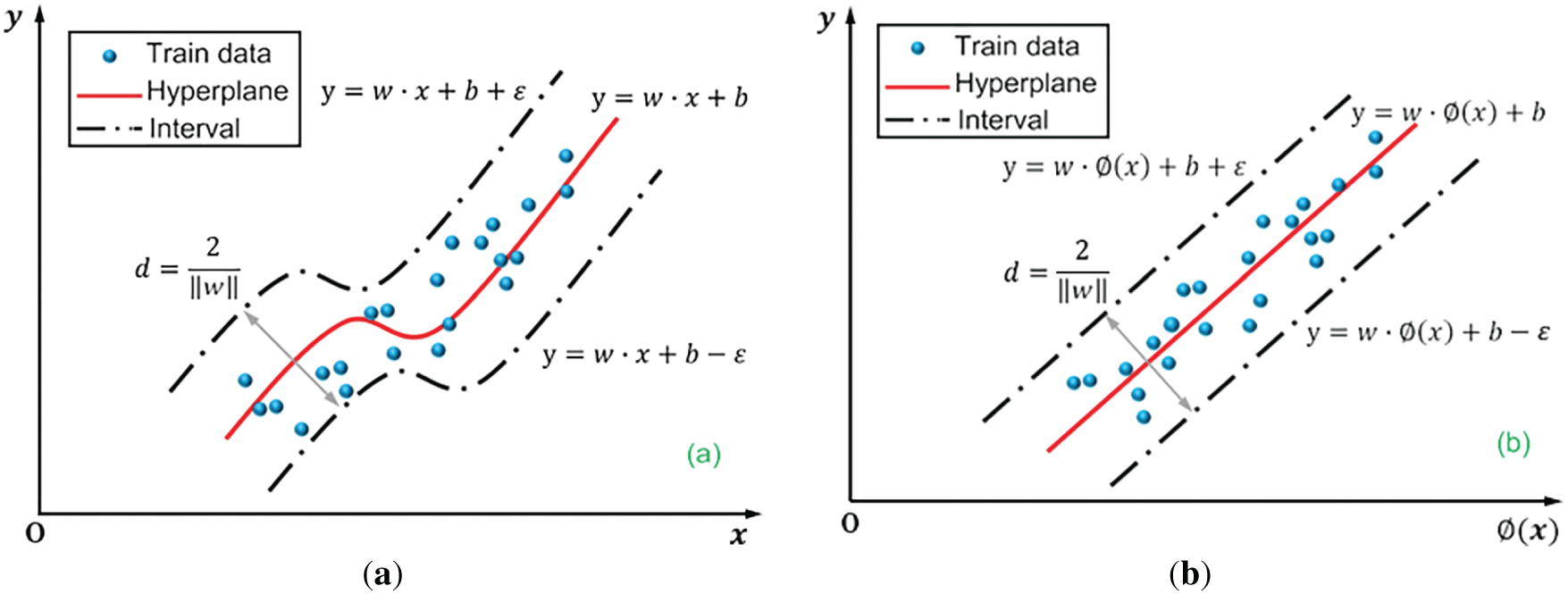
Figure 3: SVR without kernel function (a); and with kernel function (b) [30]

When SVR trains, its dual goal is to widen the margin while keeping overall loss in check. The method seeks a parameterized hyperplane that sits as far from the target points as possible, and, to facilitate learning, it allows a tolerance band where small errors are permitted. Inside that band, no penalty is counted; outside it, SVR tallies how far each point misses the mark, thus driving the final fit. Because of that band, the overall cost only climbs when predictions stray past the upper or lower limits the model has set. Formally, that mixed objective shows up in the expression given as Eq. (4) [30].

Objfunction={12w2+C∑i=1nl(yi,y^i),|y^−y|>ε12w2,|y^−y|≤ε(4)

where l is the loss function that measures the error between the predicted and true values; and C is the penalty factor for the error term.

2.3 RFR

RFR builds a group of decision trees, each trained on its randomly selected slice of the entire training set. After all the trees make their predictions, they are averaged to reach a single output. This averaging process protects the model from idiosyncratic patterns in any one sample, making it tougher and reducing overfitting. The real value of RFR can be seen when feature importance scores are examined, as they indicate which input variables contribute to increasing or decreasing Community Structure (CS) scores. Another practical advantage is that RFR ignores irrelevant or duplicated features while still delivering solid results, a helpful trait when dealing with messy, high-dimensional data sets [31]. A flow chart illustrating the RFR procedure is shown in Fig. 4. Each input batch, numbered n, carries one phenology z-score along with a year’s weather predictors for that site. From these batches, the algorithm uses bagging to create K regression trees, reshuffling the samples so that many observations appear in several trees, while others never appear at all. At each split at each tree, RFR chooses the best predictor from a smaller random pool of m features rather than from the complete set, a further source of randomness that prevents over-dependence on any individual variable. Due to these specific design elements, random forests remain steadier and more precise, and they also reduce the overlap between the regression trees within the model. Less overlap means the trees can spot a wider range of patterns in the training data. Once all K trees give their individual predictions for a new input, those values are averaged together to form the final phenology z-score estimate [32].

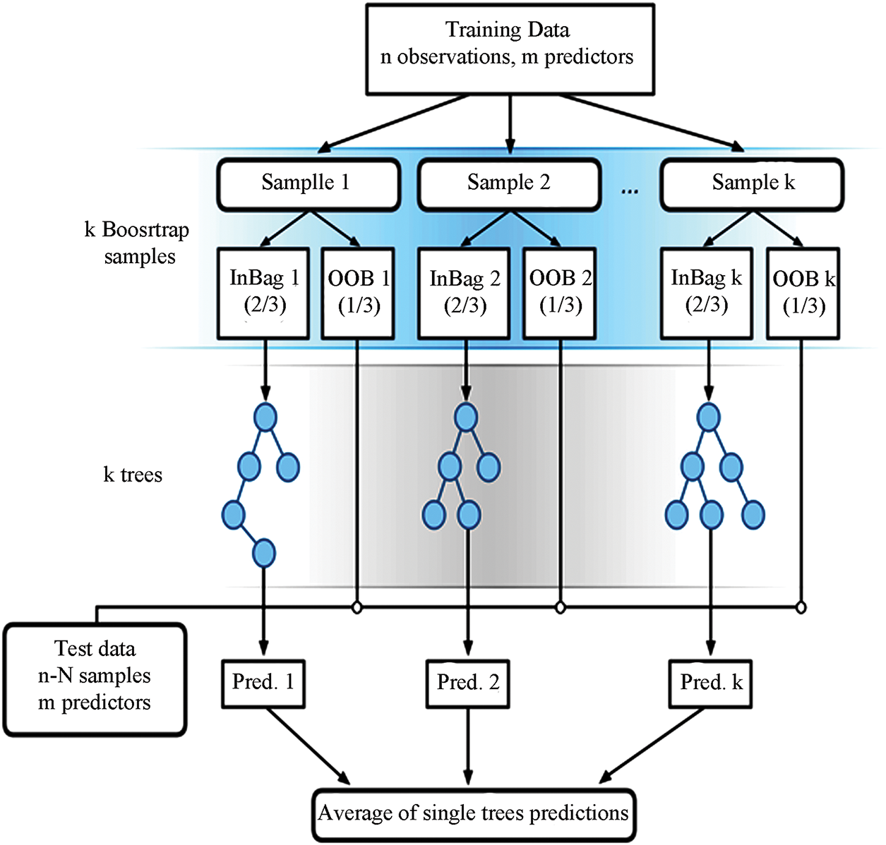
Figure 4: The flowchart of RFR [32]

2.4 XGBR

XGBR takes classic boosting a step further by adding regularization, working seamlessly with missing data, and running tasks in parallel [33]. For many practitioners, its mix of scalability and predictive punch places it near the top of the machine learning toolbox. In the current study, the model was chosen because it hunts non-linear patterns, guards against overfitting, keeps computation light, and remains interpretable [34]. The algorithm constructs a sequence of shallow decision trees, each trained to correct errors introduced by its predecessor (Fig. 5). The ensemble captures complex relationships that simple models miss by steadily shrinking the residuals. During this process, a set of internal tests grades features, guiding splits while curbing excessive growth and protecting generalization. Because users can also plug in custom loss functions, XGBR readily tackles the quirks of real-engineering tasks. Output includes a ranking of feature importance, showing developers which inputs carry the most weight. Taken together, these design choices usually yield accuracy, robustness, and a degree of insight well beyond a stand-alone weak learner [30].

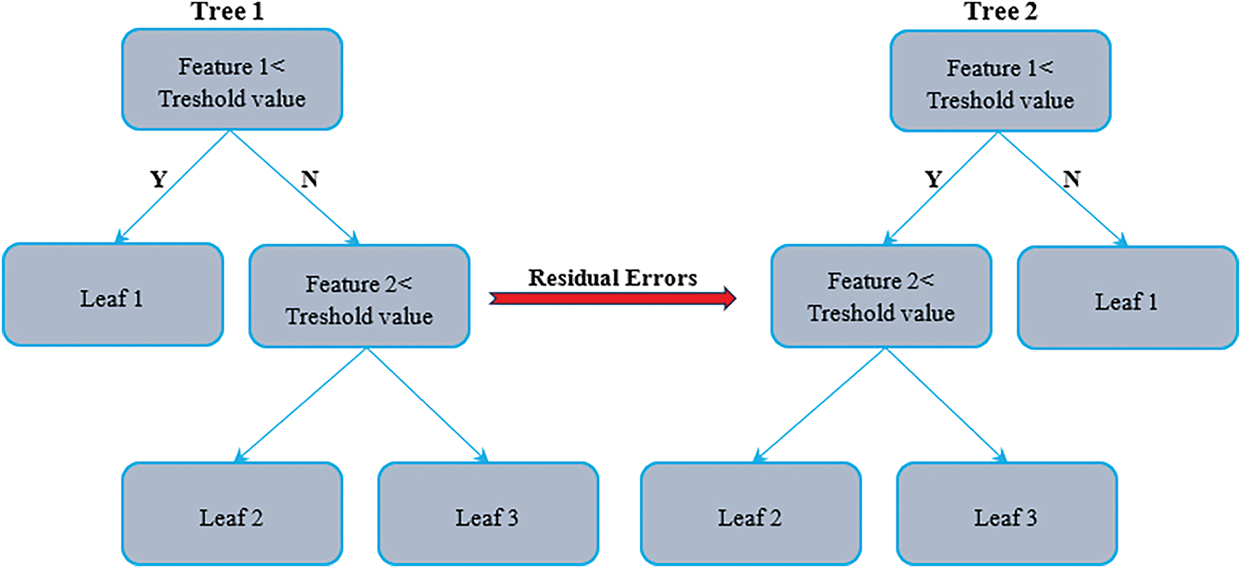
Figure 5: Schematic of XGBR [30,35,36]

2.5 KNN

A quick refresher on KNN reveals that it predicts the value of a new point by examining its K nearest neighbors in the training set. Imagine a regression task where one wants to estimate the value of a house. The KNN algorithm first identifies the K nearest houses in the stored data and then averages their sale prices to arrive at a prediction for the target house (Fig. 6). In practice, straight-line distance between each pair of houses, usually calculated with the Euclidean formula, serves as the yardstick for closeness (Eq. (5)) [30].

h=∑i=1n(xi−yi)2(5)

where x represents the target values for observed samples and y denotes the target values for neighboring samples.

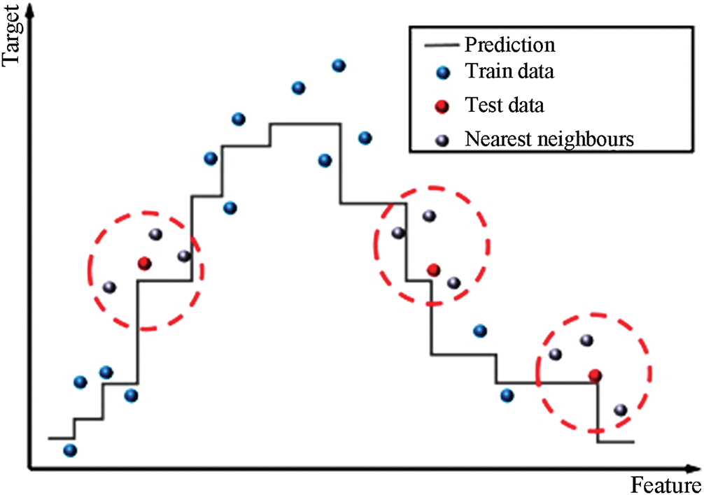
Figure 6: Schematic of KNN for regression [30]

2.6 GPR

In Bayesian inference, a Gaussian process acts as a prior over unknown functions [37]. Given N distinct non-negative integer input locations, one can build a multivariate Gaussian where the covariance is formed using the chosen kernel across these points. Drawing samples from this distribution yields function values that respect the specified covariance pattern. When faced with multi-output tasks, GPR can be scaled to handle vector-valued outputs by assembling a single large covariance matrix that encodes dependencies among both inputs and outputs [38]. This matrix-valued approach was extended to even more robust models such as Student-t processes, which feature heavier tails and are therefore more resilient to outlier observations [39]. Drawing conclusions about continuous numbers using a Gaussian process prior is known as Gaussian process regression, or GPR, and the extended version that predicts multiple outcomes simultaneously is called cokriging. Both methods provide a highly adaptable, non-linear way to fill in gaps in multivariate data, and they can be tweaked to work with mixed integer and real inputs. Beyond interpolation, Gaussian processes also appear in numerical analysis for problems such as estimating integrals, solving certain differential equations, and guiding careful, data-driven optimizations, a field sometimes referred to as probabilistic numerics [40]. Fig. 7 places GPR beside kernel ridge regression and SVR, clearly showing the unique role GPR plays. The orange GPR curve not only follows the data trend but also paints confidence bands around itself, allowing users to see how specific the model is at each point. In contrast, the red SVR line and the cyan Kernel Ridge Regression (KRR) line make bold predictions without indicating how shaky or solid those predictions are. Because of this built-in uncertainty, GPR faithfully captures tiny recurring wiggles in the data and therefore becomes indispensable in places where knowing how much to trust a forecast really matters. The GPR uses highlighted feed directly into mixture-of-experts setups. Tricky problem into smaller, familiar pieces by slicing a big, each piece is handled by its own Gaussian-process expert, together creating a clearer overall picture. Examples abound in the natural sciences, from disentangling noisy starlight in astronomy to predicting how chemical compounds behave and even to fine-tuning cost-effective surrogate models for atomic forces [41–43].

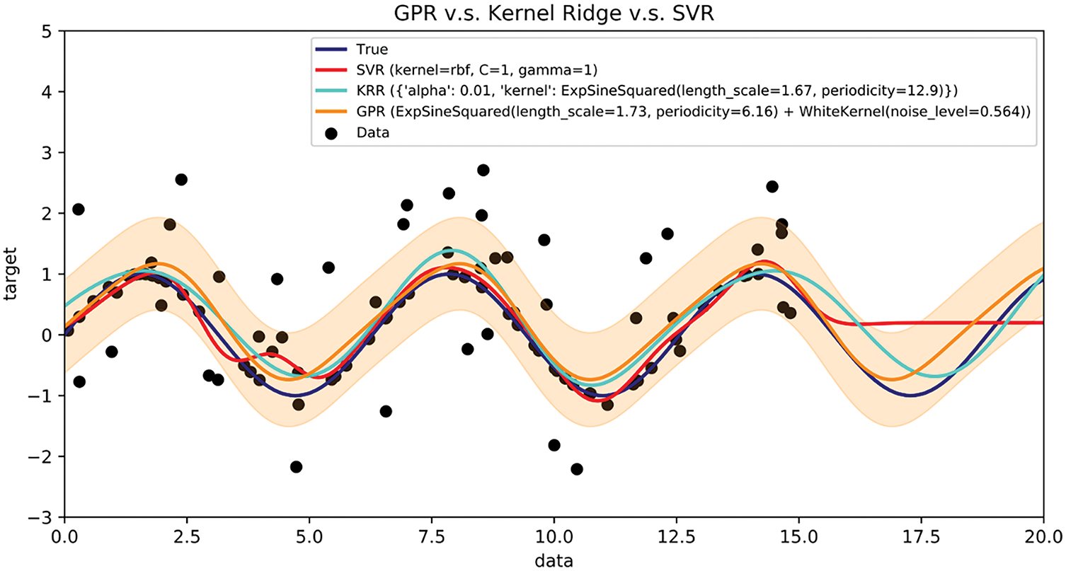
Figure 7: An example of GPR (prediction) compared to KRR and SVR [44]

3  Methodology

3.1 Concrete Sample Preparation and Fracture Energy Testing

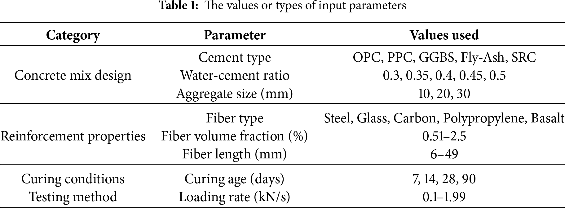
Prior to conducting laboratory tests, it is essential to set specific parameters that will employ a fracture energy influence. These parameters are concrete mix proportions, type of reinforcements, curing conditions, and loading rates. The combination of these factors enables the creation of a wide, diverse, and statistically significant dataset (Table 1). The concrete mix design comprises different types of cement, including Ordinary Portland Cement (OPC), Portland Pozzolana Cement (PPC), Ground Granulated Blast Furnace Slag (GGBS), Fly Ash cement, and Sulfate Resistant Cement (SRC). The water-to-cement ratio (W/C ratio) ranges from 0.3 to 0.5 since it affects workability, strength, and fracture toughness. Aggregates, which serve as the concrete’s bulk and provide strength, include crushed stones and river gravel in three different sizes: 10, 20, and 30 mm. Fiber reinforcement is used in the concrete mix to enhance fracture energy. The fiber types considered are five: Steel, Glass, Carbon, Polypropylene, and Basalt, with fiber volume fractions varying from 0.51% to 2.5%. The fiber lengths range from 6 to 49 mm. These changes in reinforcement properties aid in evaluating their effects on the energy needed to fracture a material and the behavior of the cracks. Various methods of curing concrete have a direct impact on strength development. The samples undergo curing at: 7, 14, 28, and 90 days under standard water curing and controlled temperature curing conditions. Different loading rates for the three-point bending test, ranging from 0.1 through to 2.0 kN/s, captures the impact of speed on fracture energy. Adjusting these parameters yields 500 data points for the study, which allows for the accurate assessment of the fracture behavior of FRC.

The three-point bending test procedure in this study follows recommendations outlined by the ACI Committee 544 (specifically ACI 544.2R-89) [45], which provides guidance for testing the flexural performance of FRC using beam specimens with a central notch. The primary objective is to ensure that the prepared concrete batches exhibit uniform characteristics, enabling meaningful comparisons of fracture energy values. All ingredients are precisely measured first, prior to the construction design guide, to set up the concrete mixture. The dry ingredients, which are cement, fine aggregate, and coarse aggregate, undergo a two-minute blending process to achieve even distribution. Gradually, superplasticizers and water are added with continued stirring for three minutes. When fibers are specified, they are added in a controlled manner to prevent balling and guarantee a uniform dispersion throughout the matrix. As a final step, the mixture was stirred for an additional two to three minutes to produce a homogeneous, fluent mixture that is workable. The blend is poured into beam molds (100 mm × 100 mm × 500 mm) after mixing. The used molds match what many labs now consider standard for testing fracture energy in FRC. This format follows guidance from the RILEM TC 50-FMC committee (1985) [46,47]. Although RILEM does not mandate a specific size, its suggestion of a 5-to-1 span-to-depth ratio and a central notch fits neatly with a 100 mm depth and a 500 mm span. The molds are first smeared with release oil to avoid sticking. The concrete is placed in three equal parts, where each part is compacted with a tamping rod or vibrating table to release air and align fibers. The upper surface is then flattened with a steel trowel for uniformity. The specimens are next left in the molds for 24 h under ambient conditions after pouring. After removal, they are immersed in water curing tanks controlled at 20°C–25°C. Using curing durations of 7, 14, 28, and 90 days, the molds are checked during these times to see how hydration periods affect fracture energy.

The measurement of fracture energy related to crack propagation is performed using a three-point bending test. This is done using a Universal Testing Machine (UTM). The UTM can support a maximum load of 100 kN, a level that comfortably handles tests on miniature FRC beams across a range of loading speeds. Its built-in load regulators and displacement sensors work together to record load-CMOD curves with the accuracy needed to calculate fracture energy reliably. Each beam specimen is placed on a pair of rollers that are 400 mm apart. A pre-notch measuring 5 mm is introduced at the center of the beam. Fill fracture occurs when a when aserves as thet serves as the the load, which is set at the midpoint to be the only load applied. The testing method involves the three steps: (1) Multiload beams are set to 0.1–2.0 kN/s to observe the effect of loading rates on fracture energy; (2) Both load and stroke are recorded during the sample processing; (3) Fracture energy of the beam specimen is gauged at its final complete fracture point.

Eq. (6) is utilized to calculate the fracture energy of concrete specimens.

GF=W/A(6)

where GF is the fracture energy, A is the total work done (the area under the load-displacement curve), and W is the fracture area (width × initial notch length).

3.2 Data Normalization and Modeling Procedure

In the context of training machine learning models, parameter normalization is critical when features have different scales or units. There are algorithms, such as those that use gradients (neural networks, support vector machines, or k-nearest neighbors), that are particularly sensitive to feature magnitudes. The dominance of value features can slow convergence and lead to skewed updates, wasting iterator cycles in the presence of large-valued features. In addition, normalization enhances numerical precision and ensures the proper functioning of distance-based models by mitigating the impact of specific features that can skew distance calculations. Normalization transforms features into a uniform range, improving the learning efficiency, stability, generalization, and overall performance of the model. A common method for normalization is Min-Max normalization, which rescales all features into a predefined range usually [0, 1] or [−1, 1]. This approach is described mathematically through Eq. (7).

X′=X−XminXmax−Xmin(7)

In this equation, X is the original feature value, and Xmin, Xmax are the minimum and maximum values of the feature, respectively. X′ is the normalized value. Under this normalization technique, which can be applied in this study, almost all parameters, such as the W/C ratio, fiber volume fraction, and loading rate, are scaled with respect to their minimum and maximum values, ensuring that all features have the same influence on the machine learning model. This modification helps enhance the stability and interpretability of the model while retaining the relationships among data points. Nonetheless, Min-Max normalization is sensitive to outliers, since outlier values tend to reduce the feature range, causing distortion. For this reason, it performs best in the absence of large anomalies within the dataset.

The Anaconda 2.3.1 environment was utilized to implement machine learning techniques through the Python programming language. This includes coding, data processing, model training, and evaluation tasks, which are performed in Jupyter Notebook 6.4.12. Jupyter Notebook is an interactive computing platform that enhances the ease of performing and visualizing experiments with complex calculations. It assists in achieving maximum productive output by allowing the flexible creation of codes, easy identification and rectification of errors, and the incorporation of numerous required Python libraries for machine learning, such as Scikit-learn, TensorFlow, NumPy, Pandas, and Matplotlib. The Anaconda distribution for Windows was selected because it provides good support for system packages and default dependencies, as well as being optimized for big data processing, which is critical in developing and improving predictive models.

3.3 Modeling Workflow

This study conducts its modeling workflow through a clear, step-by-step pipeline to ensure accurate and reproducible predictions of fracture energy in FRC. First, raw data undergoes preprocessing, in which Min-Max scaling normalizes the features, ensuring that input values fall within the same range and do not skew distance-sensitive algorithms. After scaling, the dataset is shuffled and split into training and testing sets, with 80% of the data used to train the models and 20% reserved for final performance checks. Machine learning algorithms are trained separately on the training split, and Bayesian optimization fine-tunes their hyperparameters in each case to improve generalization. Once training is complete, each model is tested not only on the held-out set but also through k-fold cross-validation, providing a more robust assessment of its predictive performance on unseen data. Results are then summarized using a battery of statistical metrics, and head-to-head comparisons reveal which model is most stable or suited to different concrete blends.

3.4 Cross-Validation Techniques

Two different cross-validation tests were conducted to ensure the model performs well on new cases and to prevent overfitting. The first step involved a simple holdout, which split the data into 80% and 20% sets, using 80% for training and the remaining 20% as an initial assessment of how well the model handled unseen examples. Hence, 5-fold cross-validation was added; the data was shuffled and split into five roughly equal groups, or folds. For each round, four of those folds trained the model, while the fifth acted as a temporary test set. The cycle continued until every observation had been tested once. The scores from all five rounds were then averaged, providing a stable and fair representation of how accurately the system will perform in real-world use. Because the fracture energy dataset is small and varies only so much, this multi-fold setup reduces random noise and provides a clearer view of model behavior.

3.5 Performance Metrics

Researchers turned to four solid statistical yardsticks: the coefficient of determination (R2), root mean squared error (RMSE), variance accounted for (VAF), and the a10-index to rigorously assess and compare how well the machine-learning models shoot their targets. R2 reveals how much of the ups and downs in the experimental fracture-energy numbers the model can explain, providing a quick read on its explanatory power. RMSE, which is tied to the scale of the actual data, indicates on average how far the predictions deviate from reality a smaller RMSE means the model is missing the mark by a narrower margin. VAF strips away some of the noise by comparing the leftover variance in the predicted and measured sets, adding yet another lens to the question of good fit. The a10-index goes a step further in an engineering context by counting the share of forecasts that land within plus-or-minus ten percent of what the lab actually recorded. Taken together, these four criteria provide a comprehensive view of accuracy, durability under varying conditions, and day-to-day trustworthiness in the model’s predictions.

4  Data Analysis

Analyzing datasets statistically helps understand their structures before operating with machine learning. Possible outcomes of missed biases, outliers, and gaps can make machine learning algorithms useless. Statistical evaluation helps to select appropriate features and assess data variability. Analysis also determines if certain assumptions, such as normality, are suitable for the algorithms in use. Descriptive statistics and correlation aids build data-driven theories, which guide decisions made during modeling. These procedures enhance the efficiency and relevance of resulting models, while increasing their applicability to new data. This study applies statistics to validate the dataset’s features, ensuring they are augmented by clean data intervals for efficient training of machine learning models.

An overview of the dataset is provided using the Pearson correlation matrix shown in Fig. 8, which illustrates the linear relationship between various attributes. The W/C ratio has a weak, but positive correlation with fracture energy at 0.077, indicating that a higher W/C ratio can improve fracture energy, albeit not by a significant margin. It is correct that raising the W/C ratio usually lowers compressive strength and fracture energy; the increased pore space and weaker bonds in the microstructure make the mix less able to resist crack growth and crack tip opening displacement (CTOD). In the dataset, the Pearson correlation between the W/C ratio and fracture energy yielded a slightly positive value of 0.077. That number does not mean that a higher W/C ratio actually improves fracture energy; it only shows a faint statistical pattern hidden among the various fiber types, volumes, lengths, and curing methods in the data. A weak positive correlation was observed in the dataset, likely because the fibers compensated for the drawbacks of a higher W/C ratio in some mixes. When W/C rises, fresh concrete becomes easier to handle, allowing the fibers to spread more evenly. This reduces clumping, raises uniform reinforcement, and helps the composite absorb energy as cracks begin. The improved distribution can also bridge tiny fissures more effectively, slightly boosting measured fracture energy even when the surrounding matrix is mechanically weaker.

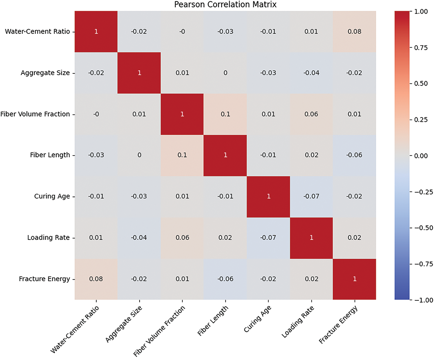
Figure 8: Heatmap of Pearson correlation matrix for the data-points

Aggregate size does not correlate with other variables, indicating its neutrality in the dataset. Fiber volume fraction and fiber length share a moderate positive correlation estimated at (0.097). This is not surprising as the properties of the fibers tend to be interconnected. Curing age shows a slightly negative correlation with loading rate, at −0.075, meaning that longer curing can reduce sensitivity due to an increase in the change in loading rate. Overall, correlations do not exhibit significant strength, indicating a high level of complexity behind these relations. Such weak and scattered correlations signify that these relationships are best described with non-linear models, as opposed to simple linear ones. One needs to use machine learning methods that work better for non-linear relationships and complex interactions to gain a better understanding of the dependencies between input parameters and fracture energy.

The boxplots given in Fig. 9 depict the distribution of five input features. Each boxplot contains an interquartile range (IQR) defined by the median values of the first and third quartiles, along with the line within the box. In addition, the whiskers illustrate the minimum and maximum values. There are no apparent outliers in any of the plots; this is a sign of well-distributed data. The symmetry in all parameters indicates a low degree of variation around the central value, which enhances the trustworthiness of these measures. The absence of variability suggests that these parameters contain no inconsistencies, making them suitable for machine learning algorithms. Since additional information and outliers can drastically affect the accuracy of predictive models, the well-organized nature of these variables ensures that more dependable models will be designed. This ensures more reliable predictions for fracture toughness and other considered properties.

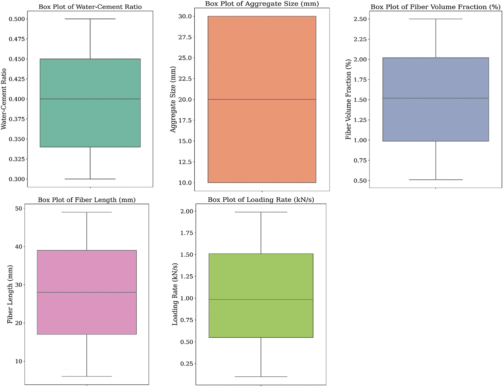
Figure 9: Box plots for numerical parameters

Due to the clear and non-continuous impact, the curing age has on concrete, as a categorical parameter. Curing age signifies specific milestone periods (7, 14, 28, and 90 days) that mark the progress of hydration and the form it takes, which, in turn, unlocks various microstructural changes and strength enhancements. These time intervals indicate thresholds in the material’s development and phases, where the speed of hydration and many other factors, such as concrete’s strength, durability, shrinkage, and numerous other properties, are not continuous but instead step-wise. Curing age as a categorical variable captures these specific effects by ensuring that all designated time points are represented and their impact on concrete performance is modeled more accurately. This reasoning aligns with the expertise in concrete technology, where practitioners analyze the behavior of concrete in relation to specific curing stages, rather than treating it as a continuous function with age as the only variable.

Fig. 10 displays count plots for the categorical parameters (cement type, fiber type, and curing age). Based on the distribution of data, GGBS and OPC appear to be the two most commonly used cement types. Fly ash, SRC, and PPC are relatively scarce, but still consistent enough to indicate a good balance within the data. For fiber type, the distribution is also balanced, with polypropylene and carbon fiber being slightly more dominant than the other types, ensuring coverage across the spectrum of fiber types. Examining the distribution of curing age as a categorical variable reveals the following observations: 7, 14, 28, and 90 days. The data is fairly consistent in terms of these categorical variables, incorporating various considerations and therefore having the potential to adequately train machine learning models. Due to the variability and diversity these parameters exhibit, complex interactions can be captured, resulting in higher model accuracy and generalization.

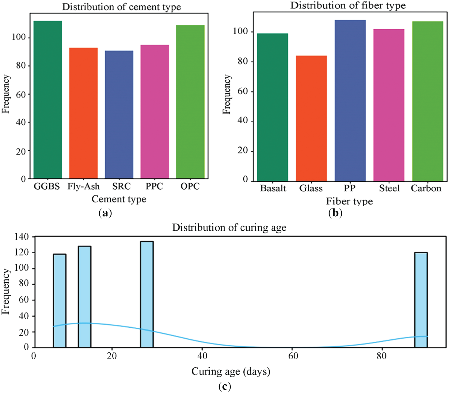
Figure 10: Count plots of categorical parameters. (a) Cement type; (b) Fiber type; (c) Curing age

Permutation Feature Importance (PFI) was employed to examine how input parameters impact fracture energy. This approach is model agnostic and provides a simple way to assess the impact of each input variable on the overall performance of the predictive model. A random forest regressor was selected for the dataset to estimate fracture energy because it is known to outperform other models, and its non-linear relationships, along with interactions between variables, make its underlying structure complex. After training, PFI was implemented by iteratively randomizing the values of individual features, disrupting their association with the target variable while maintaining the values of all other features. The model’s performance was retested after shuffling, and the performance drop highlighted the importance of that feature. A greater decrease in performance was shown to signify greater importance of the feature. A single value representing all importance scores computed from different permutations was calculated by averaging the scores along with their standard deviation to achieve robustness and reduce randomness.

Analysis of feature importance provides a clear hierarchy of the relative impact of the input parameters on the model’s output, in this case, the fracture energy. The feature importance results using the PFI method are shown in Fig. 11. Fiber volume fraction was adjudged the most vital parameter of concern for fracture energy. Increased fiber volume improves the crack-bridging mechanisms, thus enhancing the fracture resistance and total energy absorption as well as the FRC. Curing age was of lesser importance, ranked second, as longer curing periods tend to provide hydration and microstructure refinement, which increases the bond between the fibers and cement matrix, enhancing fracture energy. The W/C ratio was the third most important parameter because it affects the porosity and bonding of the matrix-fiber. A lower value of the W/C ratio is advantageous as it enhances the strength of the matrix; however, if the water content is too high, the strength of the matrix becomes weak, and energy dissipation decreases. The type of cement also significantly affected the microstructural features and how cracks propagate and energy is absorbed. Fiber length was of moderate importance, as longer fibers tend to improve crack arrest mechanisms, thus increasing fracture energy. Aggregate size was of relatively lesser importance, as the larger aggregates could form stress concentration pillars, which altered the crack path but did not significantly affect the fracture energy compared to fiber-related considerations. Fiber type has a moderate influence, as various types of fibers alter both the mechanical properties and the interaction with the matrix, changing the constituents that, in most crude forms of fracture, possess some angular merits. Amazingly, the loading rate led to some adverse effects, that is, correlates with a decrease in fracture energy. Higher loading rates typically lead to more brittle failure and less energy dissipation, which is why there is this negative influence.

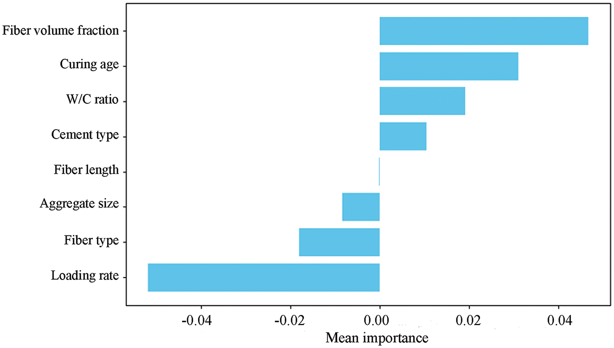
Figure 11: Feature importance results obtained using the PFI method

The sensitivity analysis reveals that the most significant variables influencing fracture energy are fiber volume fraction, curing age, and W/C ratio. Maximally tailoring these parameters in the mix design and curing processes can improve the energy absorption capacity of FRC. In addition, the adverse effect of loading rate implies that the control of the fracture-critical concrete’s loading conditions is important for high-performance designs. These results provide a reliable starting point for optimizing fracture energy in FRC through the careful selection of specific parameters and range adjustments to achieve peak performance.

Following the training of the dataset using the random forest regressor, a partial dependence plot (PDP) was developed to study the sensitivity of fracture energy to different input parameters. PDPs visually show how each input contributes to the overall output of each model, considering all other factors by averaging them out. This approach facilitates understanding of sophisticated machine learning models by illustrating how the target response (in this case, fracture energy) depends on changes in other associated features. The PDPs in Fig. 12 illustrate the relationship between fracture energy and various concrete properties. Fracture energy appears to be highly dependent on the type of cement used, as it significantly increases when the cement type changes from negative to positive values, indicating a strong dependency. The aggregate size has almost the same value, meaning it does not significantly affect the fracture energy. For fiber type, a slight non-monotonic behavior is noted, demonstrating moderate sensitivity. Moderate sensitivity is observed, as non-linear relationships are created between fracture energy and other contributing parameters. The same behavior is observed for fiber length, which yields highly variable responses, indicating a non-linear and complex relationship with fracture energy. The downward trend observed with curing age suggests that, beyond a specific point, allowing longer curing will not significantly increase fracture energy, indicating a limit. Considerable variability in bearing fracture energy highlights a complicated dependency set, which is likely impacted by the effects of strain rate within the context of fracture mechanics. The parameters that seem to matter the most in defining fracture energy are fiber volume fraction, fiber length, and loading rate, due to their pronounced non-linear effects. These parameters are likely connected to fracture mechanics in FRC because the fiber properties are crucial to the processes of crack bridging and energy dissipation. Also, the W/C ratio and type of cement used are essential since they control the microstructure and the mechanical features of the matrix. On the other hand, aggregate size, as well as curing age, appear to have lesser effects, which indicates that these parameters are either too weak or masked by fiber-associated properties.

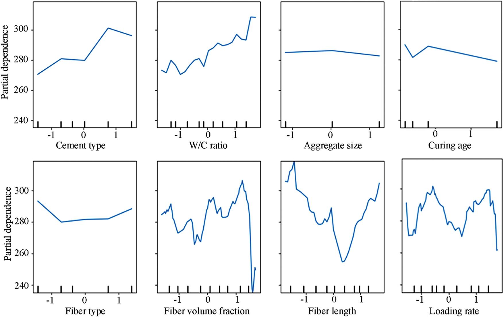
Figure 12: PDP graphs for input parameters

5  Results and Comparison

It is critical to compare different machine learning models to identify the most accurate and efficient model for a specific problem and task. For instance, in the case of predicting fracture energy, as it involves multiple parameters interacting in a complex non-linear fashion, it is not possible to assume that any single algorithm will work best without thorough testing and evaluation. Researchers need to benchmark various algorithms to determine which one best captures the complex dependencies between input parameters and output fracture energy. The benchmarking exercises serve an additional role in highlighting the performance differences among various techniques, assisting in model selection, and refinement decisions. Objective and quantifiable measurement benchmarks such as RMSE, R2, a10-index, and VAF are employed to evaluate accuracy and generalizability. A comparative study ensures that the chosen model is not only reliable but also safeguarded against dependency on specific data distributions that can mask real variability, leading to overfitting or underfitting. Most importantly, the reliability of predictions is reinforced once several models have been studied in conjunction with one another. This not only increases the clarity of machine learning applications but also enhances the interpretability of results and their utility for practical engineering work.

In the first phase of evaluating the performance of the machine learning algorithms, the holdout cross-validation technique is utilized to assess predictive power, at least for the first iteration, ensuring an accurate evaluation for each model. Following this strategy, the dataset is randomly divided into two subsets, with 80 percent of the data allocated towards training, where the models are trained to learn the patterns and relations. The remaining 20 percent of data is reserved for testing purposes, to determine how well the model generalizes its performance. This approach eliminates the problem of overfitting and ensures an unbiased estimate of accuracy for new, previously unencountered data. This approach enabled the evaluation and analysis of the effectiveness and accuracy of the machine learning models in predicting fracture energy.

In Fig. 13, a detailed examination of the fracture energy prediction within FRC is provided from the machine learning model perspective using statistical indices. Subfigure (a) presents scatter graphs of predicted vs. actual fracture energy with six models: KNN, SVR, GPR, XGBR, ANN, and RFR. The plots include annotation for perfect prediction, which is x = y, and prediction boundaries which are x = 0.9y and x = 1.1y, and the a10‐index that counts the number of predictions within the range of ±10% of actual predictions. Results indicate that the GPR model has the best a10‐index of 0.89, followed by SVR (0.86) and XGBR (0.78), confirming that these models still outperform the rest of the models. Subfigure (b) examines the performance of the models in terms of four key statistical measures. Each measure has an associated score, which increases with improved performance. GPR ranks highest overall, with a sum of scores equal to 21, as a result of its high accuracy (R2 = 0.93) and low prediction error (RMSE = 13.91). SVR, with a sum of scores of 16, emerges as the second best model, demonstrating comparable accuracy (R2 = 0.90) but higher error (RMSE = 17.14). XGBR and ANN follow closely with sums of scores of 12 and 15, respectively, indicating moderate performance across the metrics. KNN and RFR exhibited the lowest performance, scoring a total of 4 and 8, resulting from lower a10-index values and higher RMSEs. GPR outperformed the other models in all the other metrics, owing to the balance achieved between accuracy and robustness, making GPR the most suitable algorithm for predicting fracture energy in this study.

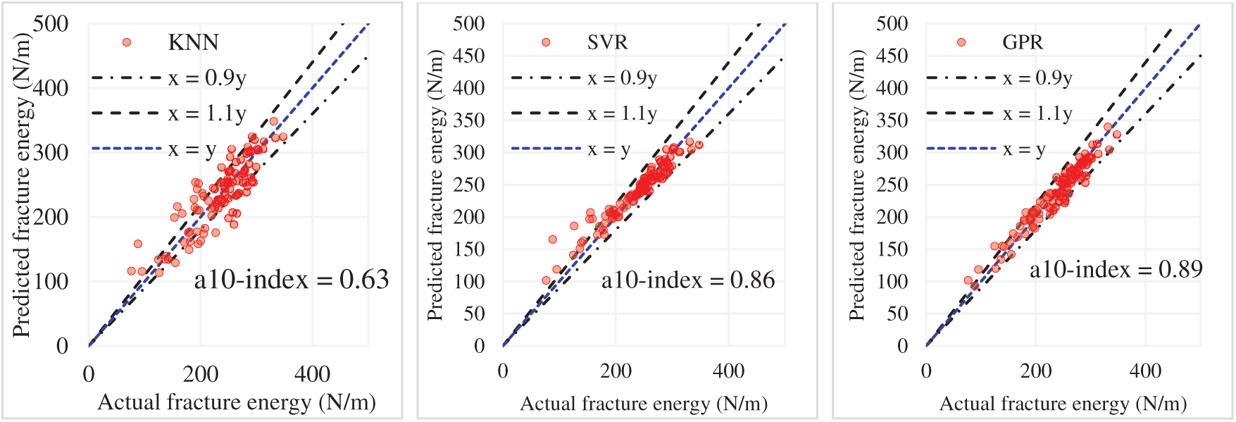
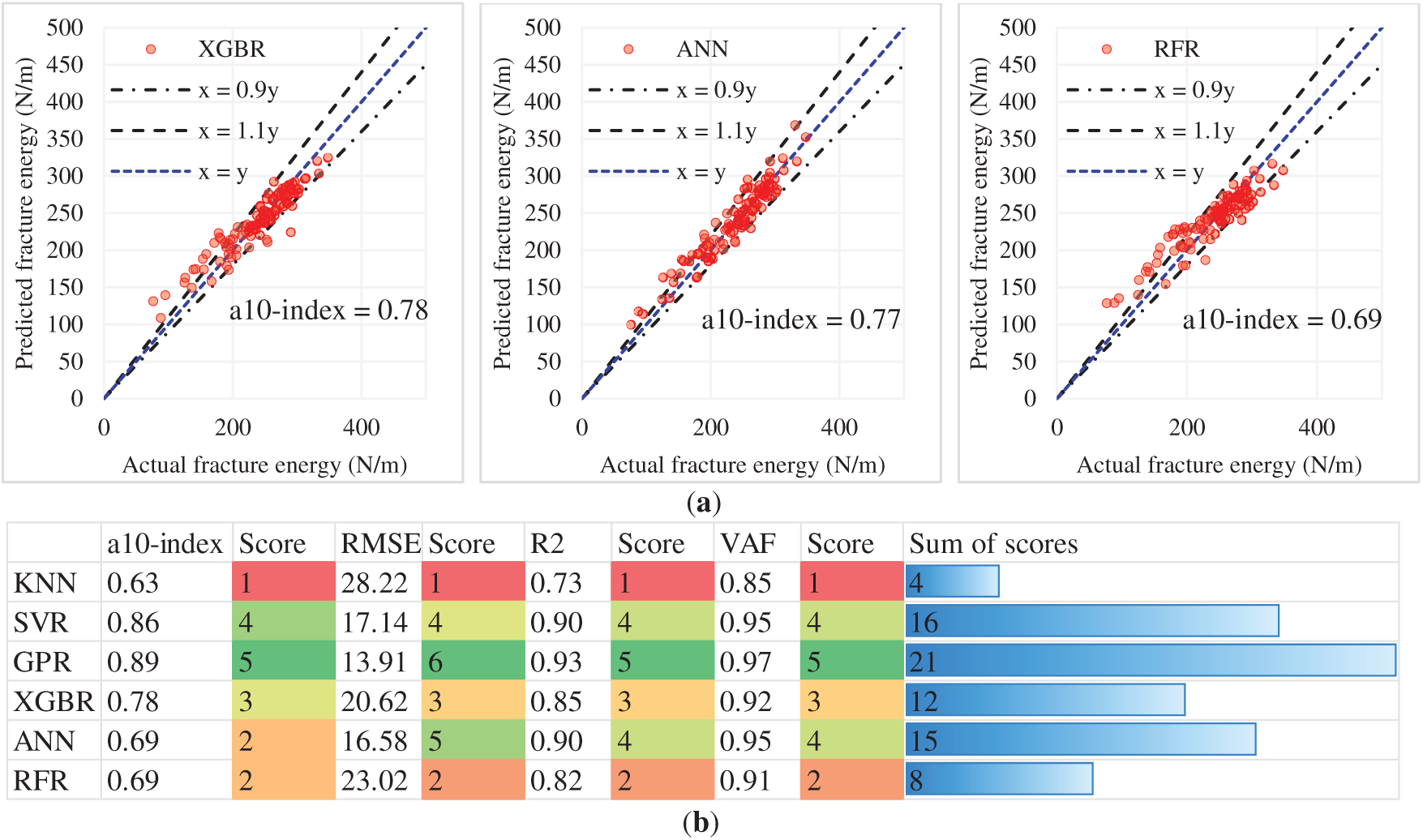
Figure 13: Comparison of holdout results obtained from algorithms through statistical indices. (a) a10‐index; (b) Comprehensive ranking score

In the second stage of the performance comparison of the algorithms, the K-fold cross-validation technique with K = 5 is used in order to enhance the reliability and robustness of the evaluation. In this method, the dataset is randomly divided into five equal-sized subsets (folds). In each iteration, four folds are used for training, while the remaining fold is used for testing. This is done five times, whereby each fold becomes the test set once, so that all data points are utilized for training and validating the model. Averaging the results of each fold computation gave a more stable and unbiased estimate of model performance. Unlike the holdout method, which splits the data once into training and testing sets, cross-validation with folds reduces the likelihood of obtaining inaccurate performance results due to a split in non-representative data. Through several training and testing cycles, K-fold cross-validation enhances the evaluation of accuracy and generalization of the model, reducing the associated variability associated with a single partitioned data split. This method is most useful with scarce datasets because it optimizes data usage and minimizes the risks of overfitting or underfitting, resulting in a more accurate assessment of the algorithm’s performance.

In Fig. 14a the GPR model is demonstrated to surpass its peers with an average R2 in excess of 0.96, minimal RMSE, and supreme VAF alongside a total score of 83, indicating GPR as the preeminent model when compared to other tested algorithms. With the GPR surpassing its score-mates with an unrivaled R2 average of over 0.96 alongside this value, the ensemble of SVR stood second with 61 points followed closely by ANN and XGBR with 45 and 55 points, respectively. The GPR performance scores exhibited consistency, enabling it to maintain an edge over its counterparts. RFR and KNN succeeded in obtaining ensemble scores that indicate a lack of predictive capabilities, outpacing comparably GPR, ANN, and SVR, which suggests a weak ability to predict trends. It is, however, interesting to note how SVR claimed the second spot, edging out RFR and KNN, which struggled with ensemble scores. Fig. 14 illustrates that both summarized and detailed views of the data chapter are incorporated to facilitate a better understanding of how peak performance is achieved, in a lift-and-look manner. The described metrics are incorporated for comparison purposes on a single unit. The GPR model relies on possessing the dependent variable data of the target, which is the current value of the GPR and boasts high ensemble performance. This model repeatedly scored high on the scoring ruler, enabling it to easily surpass its peers with the highest measuring criteria in benchmarking, capable of multiple GPR scoring overflow along multiple metrics. The bar chart in Fig. 14b supports these observations by showing that GPR has higher scores than others in every fold. However, the K-fold cross-validation approach attempts to mitigate bias or variance introduced by a static data split, ensuring a more emphatic evaluation of model validity. As the data is iteratively split into training and testing sets, the results achieved better reflect the model’s ability to generalize beyond the training set. This refinement step is essential to ensure that fracture energy prediction in FRC, where accuracy and dependability are critical, seamlessly integrates with the model selected for this analysis.

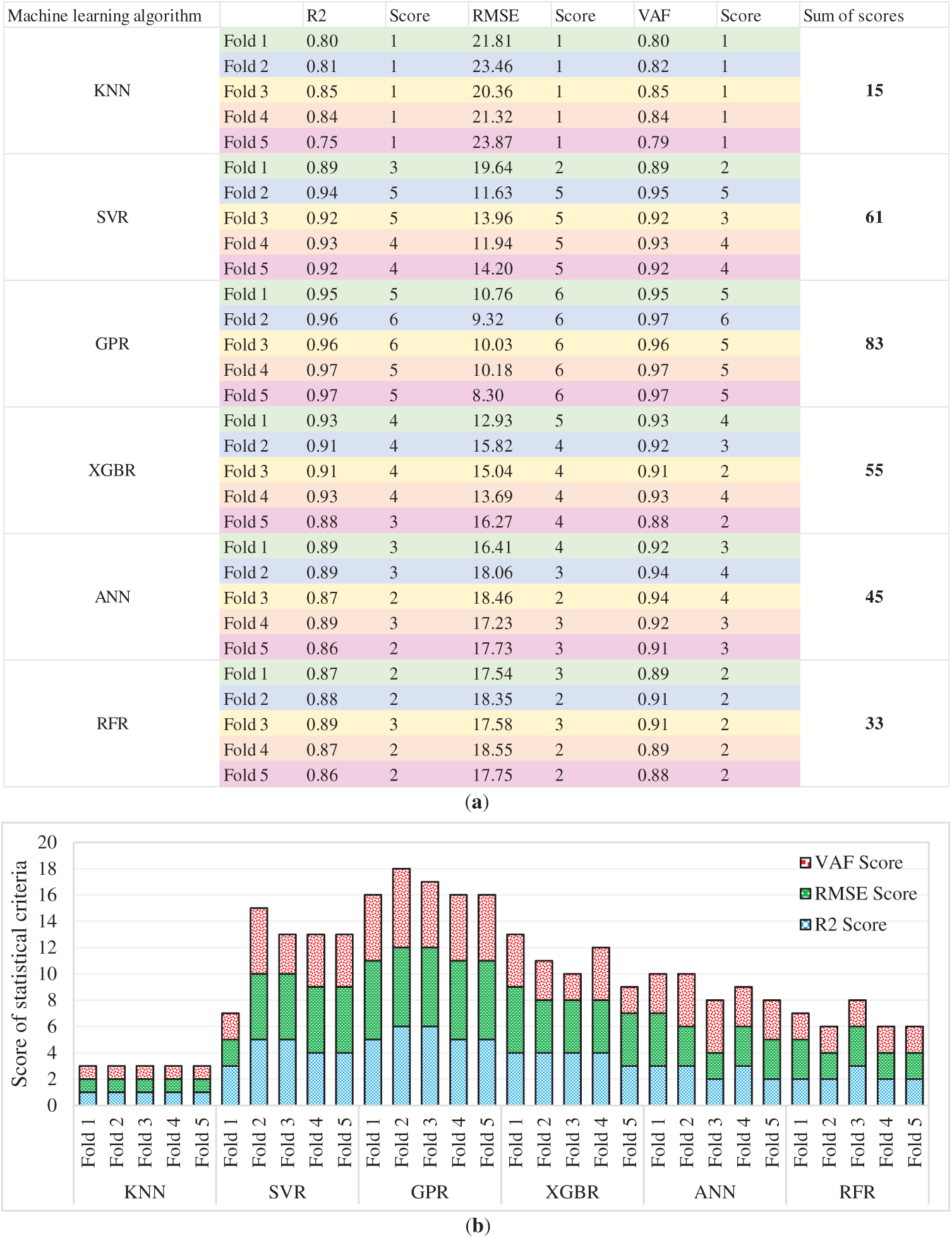
Figure 14: Comparison of the machine learning algorithms’ performance using 5-fold cross-validation: (a) tabulated results; and (b) graphical representation of the scores for each fold

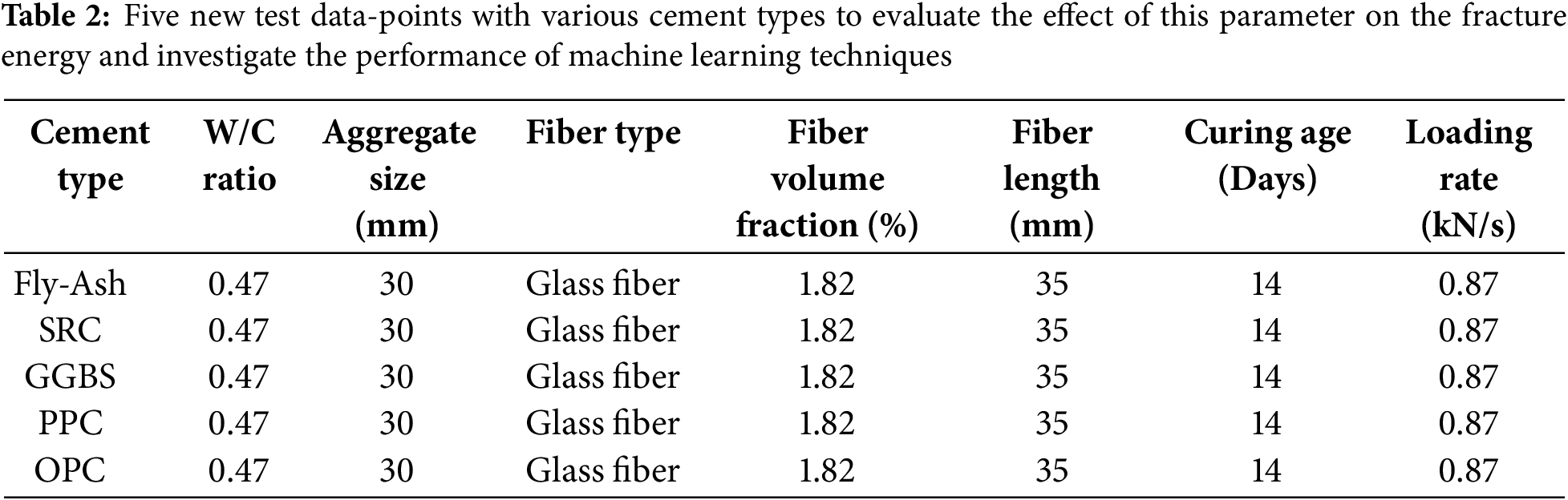
The goal now is to analyze the generalizing ability of machine learning models. Table 2 shows that five new test data points incorporate various cement types, including Fly Ash, SRC, GGBS, PPC, and OPC, while other parameters, such as the W/C ratio, aggregate size, fiber type, fiber volume fraction, fiber length, curing age, and loading rate, are kept constant. These data points are used as new benchmark tests to evaluate the extent to which a given model has achieved generalization. Actual values from three-point bending tests are shown for the fractures obtained, and predicted values from six distributed machine learning models are shown alongside. The attached graphs facilitate a visual comparison of the assumed and empirical values, which were employed to validate the estimates of the focus variable, cement type, for the fracture energy.

The comparative assessment serves as a vital evaluation of the strength and consistency of the machine learning models with respect to actual differences in concrete mix design. Since the type of cement used has a significant effect on the mechanical characteristics of the concrete, having models under such verification criteria is tantamount to an appraisal of model accuracy and generalization beyond a given dataset. The study specifically aims to develop the most dependable model for predictive fracture energy estimation, as it has significant implications in material optimization, computational modeling in civil engineering, and construction. In addition, model results that accurately align with empirical data can substantially decrease expenses and time by eliminating tedious laboratory work while still delivering dependable results. The results from the cement type parameter, denoted as Fly-Ash in Table 3, indicate that the highest amount of fracture energy is achieved when using the Fly-Ash class of cement. This indicates that Fly-Ash increases the potential energy that can be absorbed by the concrete, which is reinforced with fibers, as the fracture energy surpasses the resistance to fracture. Slow pozzolanic reactions and the formation of a permanent, dense matrix over time can also enhance the energy absorption potential of the concrete. The increase in fracture energy with the use of Fly Ash can also be justified through the positive impact of the ash on fiber-matrix interactions, which enhance the bridging mechanism of cracks, aiding in restricting their growth. In addition, these factors, along with the reduction of pores due to ash and the improved microstructure, can strengthen resistance to fractures. This shows the potential use of Fly-Ash cement class in projects needing high fracture resistance combined with durability to shift the rupture zone to severe dynamic and impact workloads on the structure.

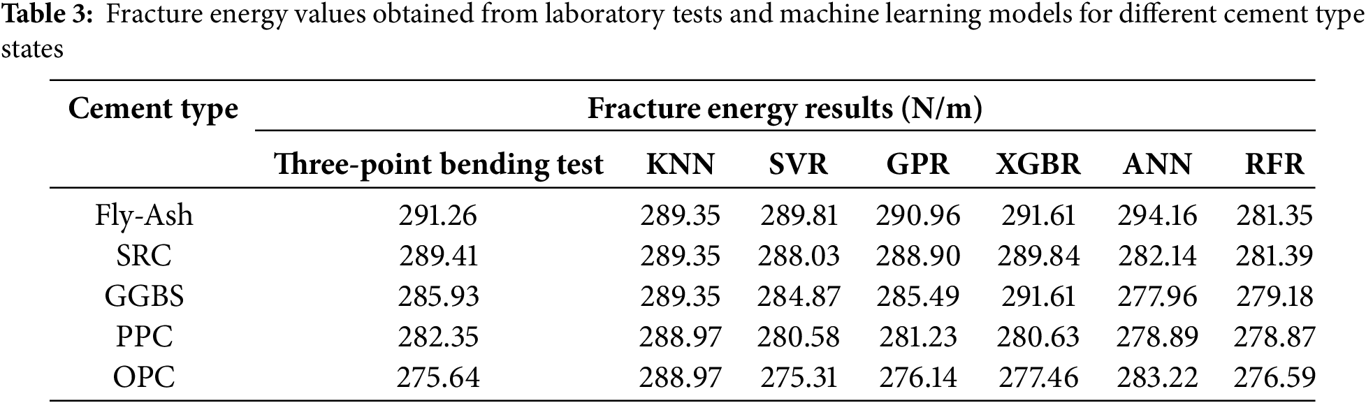
The anticipated outcomes show that GPR produces the most accurate estimates, as its predictions are in close agreement with the experimental values for all cement types tested. The SVR and XGBR models also perform competitively, though some cases showed greater discrepancies. The greatest deviation was observed in SRC, GGBS, and OPC for ANN, indicating potential overfitting or volatility in the predictions. KNN and RFR seem to underperform in most cases, implying that they do not effectively model the data for fracture energy prediction. The graphical comparison from Fig. 15 illustrates the above claims. Each graph displays laboratory test values in blue against model predictions represented by a red line. A smaller gap between the two lines indicates better model accuracy. GPR graph indicates the least deviation between predicted and actual values, demonstrating the highest accuracy. Although SVR and XGBR come closer to the predicted values, some cement types do show discrepancies. RFR and KNN do show greater deviations, but KNN is the most off-trend. Given these observations, GPR stands out as the best model in predicting fracture energy based on cement type due to its remarkable alignment with experimental data. Its versatility across various cement compositions strengthens its potential for real-world usefulness in predictive models concerning the fracture behavior of concrete structures.

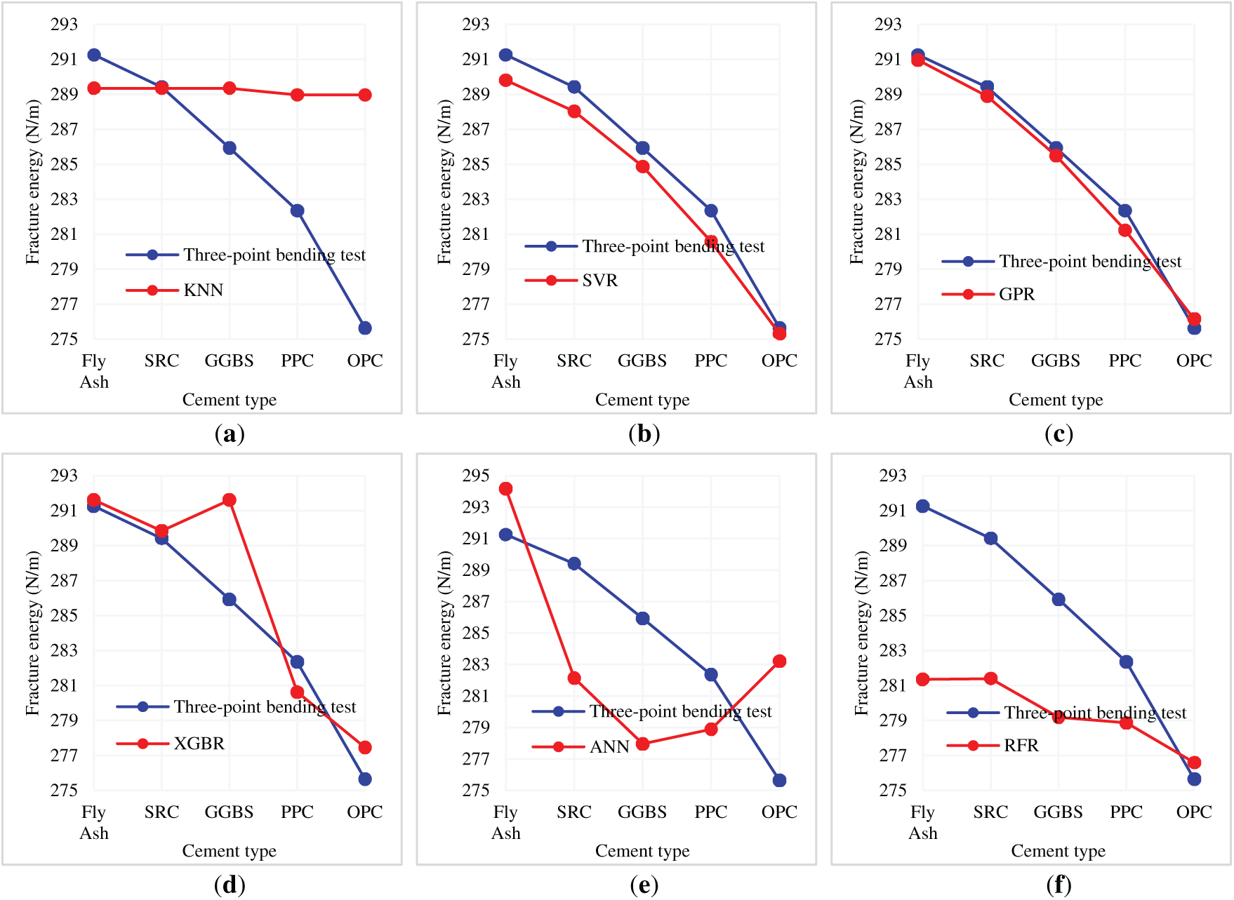
Figure 15: Comparison of fracture energy results obtained from laboratory tests and machine learning models for different cement type states. (a) KNN; (b) SVR; (c) GPR; (d) XGBR; (e) ANN; (f) RFR

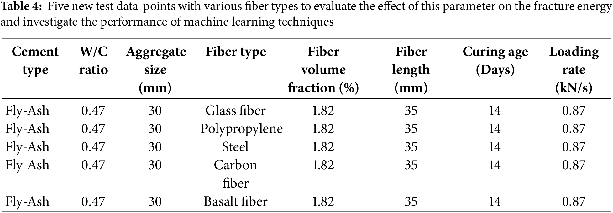
Based on Table 4, five additional test data points were added to assess the accuracy of machine learning models in predicting fracture energy relative to the fiber type employed. All other input parameters are kept constant in each case to ensure that the only change in the fracture energy calculations is due to the fiber type. The fiber types included are Glass Fiber, Polypropylene, Steel, Carbon Fiber, and Basalt Fiber, as noted in Table 4.

The fracture energy achieved through three-point bending tests is presented in each case, along with the predicted values obtained from KNN, SVR, GPR, XGBR, ANN, and RFR models, in Table 5. Table 5 exhibits that Glass Fiber showed the highest fracture energy of 291.11 N/m while Basalt Fiber was the lowest at 251.69 N/m. These differences suggest that the type of fiber reinforcement is crucial in determining fracture energy absorption and crack resistance, due to variations in bonding efficiency, fiber stiffness, and tensile strength. The value of fracture energy predicted by all the machine learning models follows the same order of reduction, which means that the models managed to capture the influence of fiber type and integrate all fracture energy parameters.

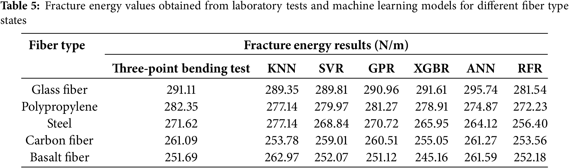
Fig. 16 illustrates how the machine learning predictions align with actual laboratory results and observations side by side. Out of all the models, GPR and SVR have the smallest deviations from the experimental values, which indicates they are the best predictors. KNN and RFR, on the other hand, demonstrate greater deviations from the experimental results, particularly for low values of fracturing energy in the Carbon Fiber and Basalt Fiber cases. This indicates that these models do not generalize well for certain types of fibers. In machine learning, this analysis highlights the significance of fiber types in determining fracturing energy, as well as their predictive capabilities regarding behaviors associated with fracturing. The performance of GPR indicates that fracture energies should be approached from a complex, non-linear perspective, most likely due to the advanced learning capabilities of such models. This is especially useful when refining the composition of FRC, as it allows engineers to select the most effective fibers required to enhance fracture resistance and predict the resistance reliably using advanced machine learning models.

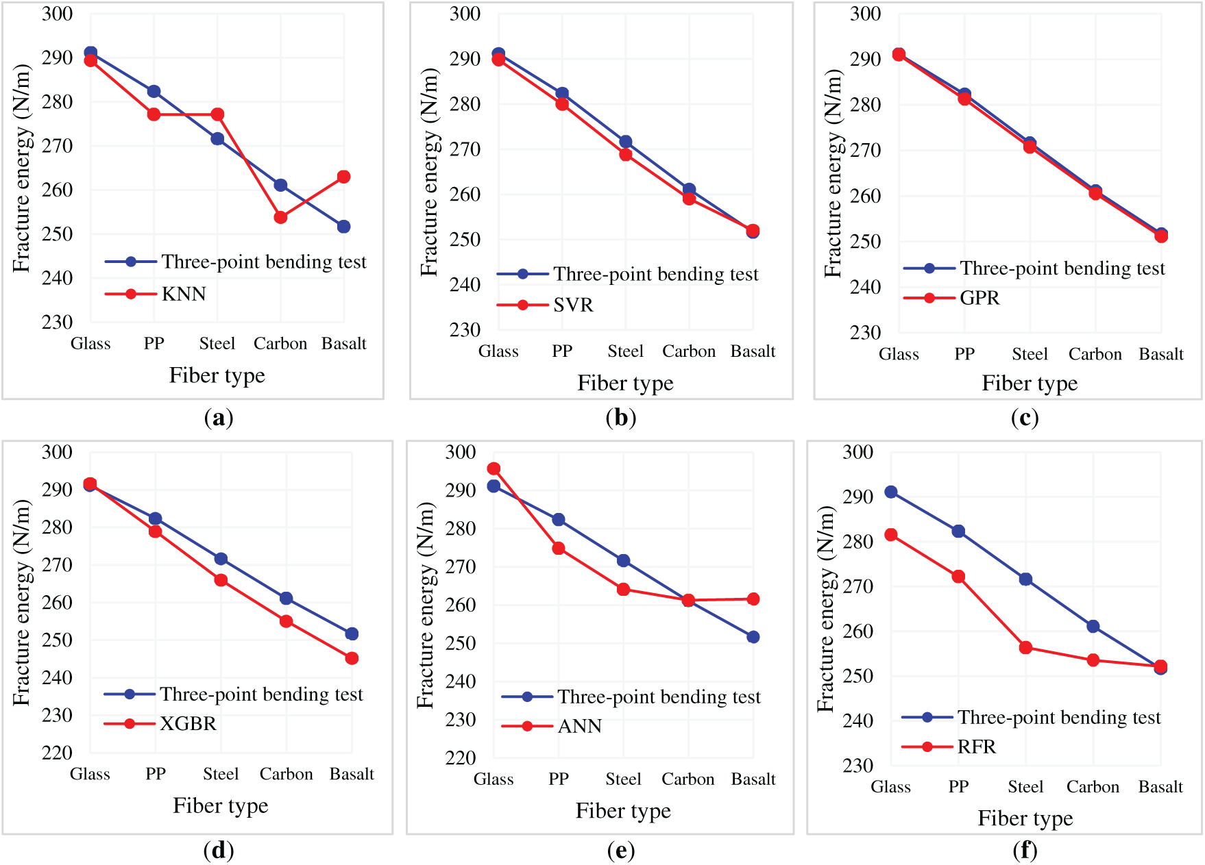
Figure 16: Comparison of fracture energy results obtained from laboratory tests and machine learning models for different fiber type states. (a) KNN; (b) SVR; (c) GPR; (d) XGBR; (e) ANN; (f) RFR

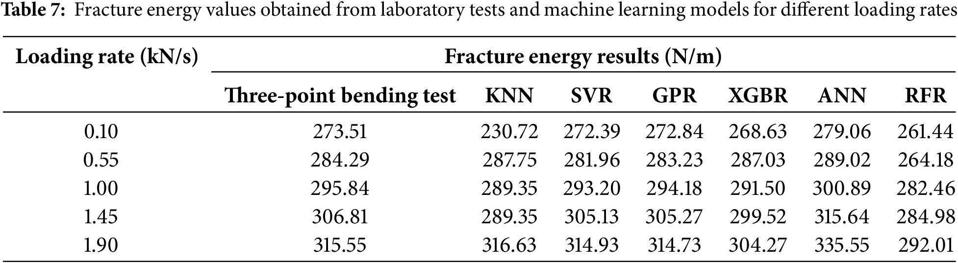
Table 6 shows that there are five additional test data points to study the effect of the loading rate on fracture energy, with the rest of the parameters unchanged. The loading rate is systematically changed from 0.10 to 1.90 kN/s, increasing by 0.45 kN/s at each step, while all other parameters remain constant.

The fracture energy values obtained from the three-point bending tests are listed in Table 7, along with the predictions made by the KNN, SVR, GPR, XGBR, ANN, and RFR models. There is a clear increasing trend in fracture energy with increasing loading rate from 273.51 N/m at 0.10 kN/s to 315.55 N/m at 1.90 kN/s. Thus, greater loading rates are somehow proportional to increased fracture energy. This is most likely caused by the rate-dependent nature of FRC, as the fibers appear to provide increased resistance at higher rates of strain.

A comparative analysis can enable the results of experiments and models through visualization in the form of graphs, as shown in Fig. 17. Fig. 17 indicates that the values predicted by the machine learning approaches provide a satisfactory result, as they seem to follow the general trend exhibited by the experimental data, reinforcing the assumption made about the relation between loading rate and fracture energy in question. Out of all the models, the best results (nearest to the experimental data) were exhibited by GPR, SVR, and XGBR, while KNN and RFR deviated from the trend too far, especially at lower loading rates, indicating some difficulty in capturing non-linear effects dependent on rate. This analysis demonstrates that higher loading rates increase fracture energy in FRC. The results further strengthen the case for incorporating strain rate effects into design and optimization procedures for concrete structures. In addition, the results demonstrate the accuracy of GPR, SVR, and XGBR models in estimating fracture energy for different loading rates, establishing them as useful predictive models for further research in fracture mechanics and concrete design.

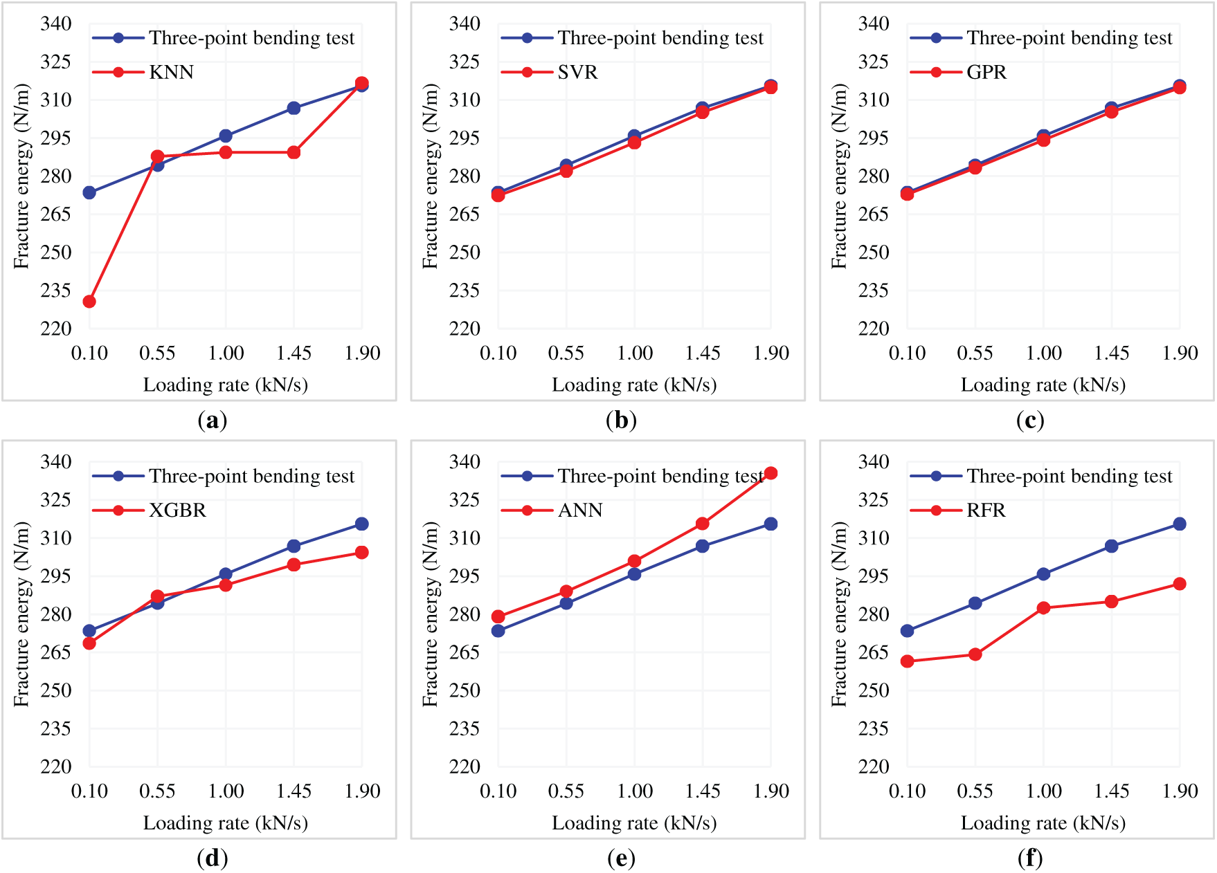
Figure 17: Comparison of fracture energy results obtained from laboratory tests and machine learning models for different loading rates. (a) KNN; (b) SVR; (c) GPR; (d) XGBR; (e) ANN; (f) RFR

The findings obtained up to now indicate that, considering the dataset employed in this study, the maximum fracture energy of concrete samples is achieved when: cement type is Fly-Ash, fiber type is glass fiber, W/C ratio is 0.50, and loading rate is set to 1.90 kN/s. In addition, the optimal parameters to achieve the highest fracture energy of FRC are not absolute and can vary depending on the values or types of parameters assumed to be constant for the purpose of this study. As mentioned previously, fracture energy in FRC is governed by several interrelated factors, including the properties of the materials, the design of the concrete mix, the interaction between the fibers and matrix, curing conditions, and test parameters. If any of the fixed parameters are changed, the optimal values of cement type, fiber type, W/C ratio, and loading rate for maximum fracture energy can change. For instance, if a volumetric fraction of fibers were altered the contribution of particular fibers to fracture energy can change, which can potentially change the order of the fibers in the ranking. A higher volume fraction of weaker fibers, such as polypropylene, can improve the performance of the fibers; however, a lower fraction can alter the performance of higher-strength fibers, such as carbon or steel. The curing conditions can also alter the hydration process and matrix bonding, which in turn can affect the impact of the W/C ratio on the fracture energy. In addition, varying loading rate ranges can alter the upper bound for energy absorption due to changes in strain rate sensitivity. Regarding optimal parameter selection, they remain constant until the dataset employed to train the machine learning models is altered. Adding new points to the dataset or re-training the model using a different sample subset can change the relationships defined based on the input parameters and fracture energy. Optimal values predicted under different distributions of the training data tend to have more iterations of the statistical dependencies present in the dataset supplied to the model. If the training dataset contains greater amounts of certain high-strength fiber types or different mix designs, the model learns different assumptions about how each parameter directly correlates with fracture energy.

Hence, in any given situation, the best parameter settings are not constant, but rather specific to that situation. Alterations in constant parameters or in the training dataset can change the optimal values of cement type, fiber type, W/C ratio, or loading rate needed to maximize fracture energy. Thus, when using machine learning techniques for predictive analysis in FRC, it is essential to ensure that the dataset used for training encompasses all relevant conditions within the application’s scope.

6  Key Limitations and Suggestions

Several key limitations of the current study will inform future investigations. One of the most important issues is the use of fixed parameters, in particular, fiber volume fraction and curing conditions, as they were fixed. This uniformity can limit the scope of the study’s findings. These parameters can be optimal for the fracture energy of certain materials, and varying the fixed values can yield different optimal parameters for fracture energy. In addition, the machine learning models are too reliant on the dataset they were trained on, meaning that if the dataset is deficient in variety regarding material properties and test conditions, then the predicting accuracy falls short. Other issues include a lack of diversity in parameter ranges; key parameters, such as fiber type, W/C ratio, and loading rate, were considered, but not aggregate type and fiber orientation, which can interact to produce crucial synergistic effects. In addition, the model overlooks the potential for not fully accounting for strain rate sensitivity in fracture energy predictions, as concrete behavior under varying loading rates tends to be non-linear and material-dependent. Lastly, predicting applicability due to the lack of generalization of machine learning models poses a problem, as these models were trained on a single dataset and multiple compositions of FRC, as well as different testing conditions, are likely to yield different results.

For future work, understanding the relationships between different parameters, such as fiber volume fractions, aggregate features, curing conditions, and types of cement, will provide a better insight into the model’s interactions and help overcome existing constraints. Including a greater variety of design configurations and fiber orientations can enhance the diversity of datasets, which in turn improves the predictive strength of machine learning models. In addition, analyzing the influence of non-linear phenomena such as rate of strain sensitivity, creep, and shrinkage, as well as dynamic load conditions, will deepen the understanding of fracture energy behavior. Incorporating other forms of machine learning, such as deep learning, ensemble learning, or hybrid techniques, can improve the accuracy of predictions by better capturing the complex dependencies between the parameters, compared to current methods. Experimental verification with various testing procedures and actual concrete structures will further validate the reliability of the predicted optimal parameters. Meeting these conditions will facilitate future attempts in machine learning applications related to predicting fracture energy and optimizing the design of FRC structures.

7  Conclusions

This study conducts a comprehensive assessment of the predictive capabilities of various machine learning models for estimating the fracture energy of FRC, ensuring multiple validations for accuracy, generalization, and consistency across different validation and testing techniques. The machine learning models are evaluated against each other with statistical benchmarks. In the holdout cross-validation (80% training, 20% testing), the GPR model yields the best results with an R2 of 0.93 and an RMSE of 13.91, alongside the best a10-index of 0.89. It is followed by SVR, with an R2 of 0.90 and an RMSE of 17.14, and XGBR, with an R2 of 0.87. KNN and RFR exhibit the weakest predictive capabilities and skew from experimental results.

A 5-fold cross-validation is also applied to improve reliability, which further confirms GPR’s superiority, with R2 values averaging above 0.96 and the highest total ranking score of 83. SVR and XGBR follow as the next best models, with scores of 61 and 55, respectively, while ANN comes with a score of 45. The robustness of the GPR model is bolstered as it repeatedly demonstrates superior performance across all folds, showing low variability and consistent stability across varying splits of training and testing data. This most consistent predictor model of FRC reveals complex non-linear relationships governing fracture energy, which is best suited to GPR in advanced applications.

Evaluation of the models is performed by validating them with new experimental data points, where one parameter is treated as a variable and the rest are held constant. As a first analysis, five test data points for different types of cement (Fly-Ash, SRC, GGBS, PPC, and OPC) are created, with other parameters kept constant. The experimental values of the fracture energy obtained through the three-point bending test are compared to the machine learning predictions. GPR proves to be the most accurate model, as it is in agreement with laboratory results for all the cement types, while SVR and XGBR are slightly off for most results. ANN also has the most issues with SRC, GGBS, and OPC, which likely means it is suffering from overfitting or some other instability. KNN and RFR yield poor results, indicating that they are ineffective in accurately modeling the fracture energy behavior with respect to different cement compositions. Results also indicated that Fly-Ash cement yields the highest fracture energy among all types due to its better fiber-matrix interaction, lower porosity, and pozzolanic reactions, which facilitate energy absorption and crack bridging. In the next step, the effect of fiber type on fracture energy is analyzed. The results indicated that glass fiber has the highest value of fracture energy and basalt has the lowest. This discrepancy arises from the mechanical differences of the fibers, including their tensile strength, bond to the cement matrix, and energy dissipation characteristics. The trends are encapsulated by the machine learning models, where the GPR and SVR predictions are most accurate compared to KNN and RFR, which showed more divergence. In the following step, the W/C ratio is investigated, starting from 0.3 to 0.5, with increments of 0.05, while fixing all other mix design parameters. The outcome showed a marked improvement in fracture energy with an increase in W/C ratio to 0.5, from 232.58 N/m at 0.3 to 298.74 N/m at 0.5. This pattern can be explained by workability and matrix-fiber bond at higher W/C ratios, resulting in improved energy dissipation within the fracture. The relationship is captured well by the GPR and SVR predictions, while the RFR model shows significantly higher discrepancies compared to the other models at lower W/C ratios. In addition, the impact of the loading rate is examined systematically by varying it between 0.10 and 1.90 kN/s. There is a positive relationship between loading rate and fracture energy since fracture energy at 0.10 kN/s was 273.51 N/m and at 1.90 kN/s it is 315.55 N/m. The reason for this behavior can be attributed to the strain-rate sensitivity of fiber-reinforced composites, where at higher strain rates, the bridging effects and energy absorption of the fibers are greater. The machine learning models, for the most part, predict these trends accurately, with GPR and SVR being the most dependable, while KNN and RFR deviate slightly from the prediction at the highest and lowest loading rates.

In general, combining machine learning approaches with experimental data related to predicting fracture energy yields accurate results. GPR demonstrates the best predictive results over all models, followed by SVR and ANN. KNN and RFR, though, present slightly higher errors in some instances, more so than expected. This study reveals that the cement type, fiber type, W/C ratio, and loading rate have significant impacts on fracture energy, which informs optimizations in mix designs of FRC for improved mechanical properties. This enables the use of data-driven techniques in fracture mechanics, structural design, and the optimization of fiber-reinforced composites for engineering applications.

The parameters that a refined analysis of the data suggested are best for achieving the maximum fracture energy in FRC structures were: Fly-Ash cement, Glass fiber, a W/C ratio of 0.50, and a loading rate of 1.90 kN/s. It is critical to highlight, however, that these parameters, as stated above, are not fixed and can change based on study factors since, as previously pointed out, fracture energy is controlled by several factors, which include: the material properties, mix design, interfacial fiber-matrix interactions, curing conditions, and other test parameters. Some fixed parameter changes, such as the fiber volume fraction or the curing process, can impact the optimal parameters. In addition, machine learning models depend on patterns within dataset, meaning the optimal values can shift if different training data distributions were used. For this reason, it is accurate to say that ideal parameter choice is context-dependent, and without a guarantee of accuracy from machine learning in FRC applications, a dataset needs to be carefully curated. Based on the analysis results, however, it appears feasible to conclude that, at least with the aid of machine learning models, an optimal mixing design can be generated, resulting in concrete samples with maximum fracture energy.

Acknowledgement: The author would like to thank Prince Sultan University for their support. Princess Nourah Bint Abdulrahman University Researchers Supporting Project number (PNURSP2025R300). This study is supported via funding from Prince Sattam Bin Abdulaziz University project number (PSAU/2025/R/1447).

Funding Statement: The author would like to thank Prince Sultan University for their support. Princess Nourah Bint Abdulrahman University Researchers Supporting Project number (PNURSP2025R300). This study is supported via funding from Prince Sattam Bin Abdulaziz University project number (PSAU/2025/R/1447).

Author Contributions: The authors confirm contribution to the paper as follows: Conceptualization, Ala’a R. Al-Shamasneh and Faten Khalid Karim; methodology, Arsalan Mahmoodzadeh; software, Arsalan Mahmoodzadeh; validation, Ala’a R. Al-Shamasneh, Faten Khalid Karim, and Arsalan Mahmoodzadeh; formal analysis, Arsalan Mahmoodzadeh; investigation, Arsalan Mahmoodzadeh; resources, Arsalan Mahmoodzadeh and Abdulaziz Alghamdi; data curation, Arsalan Mahmoodzadeh; writing—original draft preparation, Arsalan Mahmoodzadeh; writing—review and editing, Arsalan Mahmoodzadeh, Abdullah Alqahtani, and Abed Alanazi; visualization, Arsalan Mahmoodzadeh; supervision, Ala’a R. Al-Shamasneh and Abdullah Alqahtani; project administration, Ala’a R. Al-Shamasneh and Abed Alanazi; funding acquisition, Ala’a R. Al-Shamasneh and Shtwai Alsubai. All authors reviewed the results and approved the final version of the manuscript.

Availability of Data and Materials: Data not available due to restrictions imposed by research sponsors, ongoing analysis for future studies, and the necessity to maintain data confidentiality until further validation and publication.

Ethics Approval: This study did not involve any human participants, animals, or sensitive personal data. Therefore, ethics approval was not required in accordance with institutional and national guidelines. All experimental procedures were conducted in compliance with standard laboratory protocols and safety regulations.

Conflicts of Interest: The authors declare no conflicts of interest to report regarding the present study.

References

1. Monazami M, Gupta R. Investigation of mechanical behavior and fracture energy of fiber-reinforced concrete beams and panels. Cem Concr Compos. 2022;133(2):104656. doi:10.1016/j.cemconcomp.2022.104656. [Google Scholar] [CrossRef]

2. Han X, Wang H, Gao H, Zheng J, Yu RC, Wang Z, et al. Fracture energy of concrete after sustained loading. Eng Fract Mech. 2024;308(21):110350. doi:10.1016/j.engfracmech.2024.110350. [Google Scholar] [CrossRef]

3. Karimi HR, Aliha MRM, Ebneabbasi P, Salehi SM, Khedri E, Haghighatpour PJ. Mode I and mode II fracture toughness and fracture energy of cement concrete containing different percentages of coarse and fine recycled tire rubber granules. Theor Appl Fract Mech. 2023;123:103722. doi:10.1016/j.tafmec.2022.103722. [Google Scholar] [CrossRef]

4. Abolhasani A, Shakouri M, Dehestani M, Samali B, Banihashemi S. A comprehensive evaluation of fracture toughness, fracture energy, flexural strength and microstructure of calcium aluminate cement concrete exposed to high temperatures. Eng Fract Mech. 2022;261(11):108221. doi:10.1016/j.engfracmech.2021.108221. [Google Scholar] [CrossRef]

5. Dabbaghi F, Fallahnejad H, Nasrollahpour S, Dehestani M, Yousefpour H. Evaluation of fracture energy, toughness, brittleness, and fracture process zone properties for lightweight concrete exposed to high temperatures. Theor Appl Fract Mech. 2021;116(3):103088. doi:10.1016/j.tafmec.2021.103088. [Google Scholar] [CrossRef]

6. Bazant ZP, Planas J. Fracture and size effect in concrete and other quasibrittle materials. New York, NY, USA: Routledge; 2019. [Google Scholar]

7. Mobasher B. Mechanics of fiber and textile reinforced cement composites. Boca Raton, FL, USA: CRC Press; 2011. doi:10.1201/b11181. [Google Scholar] [CrossRef]

8. Malvar LJ, Warren GE. Fracture energy for three-point-bend tests on single-edge-notched beams. Exp Mech. 1988;28(3):266–72. doi:10.1007/BF02329022. [Google Scholar] [CrossRef]

9. Guan J, Hu X, Li Q. In-depth analysis of notched 3-p-b concrete fracture. Eng Fract Mech. 2016;165(3):57–71. doi:10.1016/j.engfracmech.2016.08.020. [Google Scholar] [CrossRef]

10. Karihaloo BL, Nallathambi P. Fracture toughness of plain concrete from three-point bend specimens. Mater Struct. 1989;22(3):185–93. doi:10.1007/BF02472186. [Google Scholar] [CrossRef]

11. Nikbin IM, Rahimi RS, Allahyari H. A new empirical formula for prediction of fracture energy of concrete based on the artificial neural network. Eng Fract Mech. 2017;186:466–82. doi:10.1016/j.engfracmech.2017.11.010. [Google Scholar] [CrossRef]

12. Albaijan I, Fakhri D, Hussein Mohammed A, Mahmoodzadeh A, Hashim Ibrahim H, Babeker Elhag A, et al. Several machine learning models to estimate the effect of an acid environment on the effective fracture toughness of normal and reinforced concrete. Theor Appl Fract Mech. 2023;126(10):103999. doi:10.1016/j.tafmec.2023.103999. [Google Scholar] [CrossRef]

13. Albaijan I, Mahmoodzadeh A, Hussein Mohammed A, Mohammadi M, Gutub S, Mutab Alsalami O, et al. Estimating the initial fracture energy of concrete using various machine learning techniques. Eng Fract Mech. 2024;295(9):109776. doi:10.1016/j.engfracmech.2023.109776. [Google Scholar] [CrossRef]

14. Arif M, Jan F, Rezzoug A, Ali Afridi M, Luqman M, Khan WA, et al. Data-driven models for predicting compressive strength of 3D-printed fiber-reinforced concrete using interpretable machine learning algorithms. Case Stud Constr Mater. 2024;21(4):e03935. doi:10.1016/j.cscm.2024.e03935. [Google Scholar] [CrossRef]

15. Wei Y, Chen P, Cao S, Wang H, Liu Y, Wang Z, et al. Prediction of carbonation depth for concrete containing mineral admixtures based on machine learning. Arab J Sci Eng. 2023;48(10):13211–25. doi:10.1007/s13369-023-07645-8. [Google Scholar] [CrossRef]

16. Chen T. Machine learning based grey wolf optimal controller of modified algorithm for reinforced concrete structures. Comput Concr. 2024;34(6):649–57. doi:10.12989/cac.2024.34.6.649. [Google Scholar] [CrossRef]

17. Kang MC, Yoo DY, Gupta R. Machine learning-based prediction for compressive and flexural strengths of steel fiber-reinforced concrete. Constr Build Mater. 2021;266(6):121117. doi:10.1016/j.conbuildmat.2020.121117. [Google Scholar] [CrossRef]

18. Tran VQ, Dang VQ, Ho LS. Evaluating compressive strength of concrete made with recycled concrete aggregates using machine learning approach. Constr Build Mater. 2022;323(2):126578. doi:10.1016/j.conbuildmat.2022.126578. [Google Scholar] [CrossRef]

19. Khan K, Ahmad W, Amin MN, Ahmad A, Nazar S, Alabdullah AA. Compressive strength estimation of steel-fiber-reinforced concrete and raw material interactions using advanced algorithms. Polymers. 2022;14(15):3065. doi:10.3390/polym14153065. [Google Scholar] [CrossRef]

20. Zhang J, Li D, Wang Y. Toward intelligent construction: prediction of mechanical properties of manufactured-sand concrete using tree-based models. J Clean Prod. 2020;258(9):120665. doi:10.1016/j.jclepro.2020.120665. [Google Scholar] [CrossRef]

21. Tarawneh A, Saleh E, Almasabha G, Alghossoon A. Hybrid data-driven machine learning framework for determining prestressed concrete losses. Arab J Sci Eng. 2023;48(10):13179–93. doi:10.1007/s13369-023-07714-y. [Google Scholar] [CrossRef]

22. Xiao Q, Li C, Lei S, Han X, Chen Q, Qiu Z, et al. Using hybrid artificial intelligence approaches to predict the fracture energy of concrete beams. Adv Civ Eng. 2021;2021(1):6663767. doi:10.1155/2021/6663767. [Google Scholar] [CrossRef]

23. Tran NT, Nguyen TK, Nguyen DL, Le QH. Assessment of fracture energy of strain-hardening fiber-reinforced cementitious composite using experiment and machine learning technique. Struct Concr. 2023;24(3):4185–98. doi:10.1002/suco.202200332. [Google Scholar] [CrossRef]

24. Kumar R, Rai B, Samui P. Machine learning techniques for prediction of failure loads and fracture characteristics of high and ultra-high strength concrete beams. Innov Infrastruct Solut. 2023;8(8):219. doi:10.1007/s41062-023-01191-w. [Google Scholar] [CrossRef]

25. Wang H, Zhang W, Lin J, Guo S. Research on fracture energy prediction and size effect of concrete based on deep learning with SHAP interpretability method. Buildings. 2025;15(13):2149. doi:10.3390/buildings15132149. [Google Scholar] [CrossRef]

26. Kewalramani M, Samadi H, Mahmoodzadeh A, Ghazouani N, Alghamdi A, Albaijan I, et al. Prediction of initial fracture energy governing crack propagation in concrete specimens using hybrid machine learning and empirical approaches. Steel Compos Struct. 2025;55(3):191–210. doi:10.12989/scs.2025.55.3.191. [Google Scholar] [CrossRef]

27. McCulloch WS, Pitts W. A logical calculus of the ideas immanent in nervous activity. Bull Math Biophys. 1943;5(4):115–33. doi:10.1007/BF02478259. [Google Scholar] [CrossRef]

28. Zhang Q, Yu H, Barbiero M, Wang B, Gu M. Artificial neural networks enabled by nanophotonics. Light Sci Appl. 2019;8(1):42. doi:10.1038/s41377-019-0151-0. [Google Scholar] [PubMed] [CrossRef]

29. Cortes C, Vapnik V. Support-vector networks. Mach Learn. 1995;20(3):273–97. doi:10.1007/BF00994018. [Google Scholar] [CrossRef]

30. Li L, Zuo L, Wei G, Jiang S, Yu J. A stacking machine learning model for predicting pullout capacity of small ground anchors. AI Civ Eng. 2024;3(1):11. doi:10.1007/s43503-024-00032-8. [Google Scholar] [CrossRef]

31. Ho TK. The random subspace method for constructing decision forests. IEEE Trans Pattern Anal Machine Intell. 1998;20(8):832–44. doi:10.1109/34.709601. [Google Scholar] [CrossRef]

32. Rodriguez-Galiano VF, Sanchez-Castillo M, Dash J, Atkinson PM, Ojeda-Zujar J. Modelling interannual variation in the spring and autumn land surface phenology of the European forest. Biogeosciences. 2016;13(11):3305–17. doi:10.5194/bg-13-3305-2016. [Google Scholar] [CrossRef]

33. Chen T, Guestrin C. XGBoost: a scalable tree boosting system. In: Proceedings of the 22nd ACM SIGKDD International Conference on Knowledge Discovery and Data Mining; 2016 Aug 13–17; San Francisco, CA, USA. p. 785–94. doi:10.1145/2939672.2939785. [Google Scholar] [CrossRef]

34. Dehestani A, Kazemi F, Abdi R, Nitka M. Prediction of fracture toughness in fibre-reinforced concrete, mortar, and rocks using various machine learning techniques. Eng Fract Mech. 2022;276(4):108914. doi:10.1016/j.engfracmech.2022.108914. [Google Scholar] [CrossRef]

35. Dong W, Huang Y, Lehane B, Ma G. XGBoost algorithm-based prediction of concrete electrical resistivity for structural health monitoring. Autom Constr. 2020;114(8):103155. doi:10.1016/j.autcon.2020.103155. [Google Scholar] [CrossRef]

36. Dong X, Yu Z, Cao W, Shi Y, Ma Q. A survey on ensemble learning. Front Comput Sci. 2020;14(2):241–58. doi:10.1007/s11704-019-8208-z. [Google Scholar] [CrossRef]

37. Rasmussen CE. Gaussian processes in machine learning. In: Advanced lectures on machine learning. Berlin/Heidelberg, Germany: Springer; 2004. p. 63–71. doi:10.1007/978-3-540-28650-9_4. [Google Scholar] [CrossRef]

38. Álvarez MA, Rosasco L, Lawrence ND. Kernels for vector-valued functions: a review. FNT Mach Learn. 2012;4(3):195–266. doi:10.1561/2200000036. [Google Scholar] [CrossRef]

39. Chen Z, Wang B, Gorban AN. Multivariate Gaussian and Student-t process regression for multi-output prediction. Neural Comput Appl. 2020;32(8):3005–28. doi:10.1007/s00521-019-04687-8. [Google Scholar] [CrossRef]

40. Saves P, Diouane Y, Bartoli N, Lefebvre T, Morlier J. A mixed-categorical correlation kernel for Gaussian process. Neurocomputing. 2023;550:126472. doi:10.1016/j.neucom.2023.126472. [Google Scholar] [CrossRef]

41. Chatzis SP. A latent variable Gaussian process model with Pitman-Yor process priors for multiclass classification. Neurocomputing. 2013;120(3):482–9. doi:10.1016/j.neucom.2013.04.029. [Google Scholar] [CrossRef]

42. Shanks BL, Sullivan HW, Shazed AR, Hoepfner MP. Accelerated Bayesian inference for molecular simulations using local Gaussian process surrogate models. J Chem Theory Comput. 2024;20(9):3798–808. doi:10.1021/acs.jctc.3c01358. [Google Scholar] [PubMed] [CrossRef]

43. Platanios EA, Chatzis SP. Gaussian process-mixture conditional heteroscedasticity. IEEE Trans Pattern Anal Mach Intell. 2014;36(5):888–900. doi:10.1109/tpami.2013.183. [Google Scholar] [PubMed] [CrossRef]

44. Wikipedia. Gaussian process. [cited 2025 Aug 1]. Available from: https://en.wikipedia.org/wiki/Gaussian_process#cite_note-23. [Google Scholar]

45. ACI Committee 544. 544.2R-89: measurement of properties of fiber reinforced concrete. Farmington Hills, MI, USA: American Concrete Institute; 2002. [Google Scholar]

46. Karihaloo BL, Nallathambi P. Test methods for determining mode I fracture toughness of concrete. In: Toughening mechanisms in quasi-brittle materials. Dordrecht, The Netherlands: Springer; 1991. p. 91–124. doi: 10.1007/978-94-011-3388-3_7. [Google Scholar] [CrossRef]

47. Determination of the fracture energy of mortar and concrete by means of three-point bend tests on notched beams. Mater Struct. 1985;18(4):287–90. doi:10.1007/BF02472918. [Google Scholar] [CrossRef]