
 Submit a Paper
 Propose a Special lssue
 Open Access
ARTICLE
Hybrid Wavelet Methods for Nonlinear Multi-Term Caputo Variable-Order Partial Differential Equations
1 Department of Mathematical Sciences, Ulsan National Institute of Science and Technology, Ulsan, 44919, Republic of Korea
2 NUST Institute of Civil Engineering, School of Civil and Environmental Engineering, National University of Sciences and Technology (NUST), Sector H-12, Islamabad, 44000, Pakistan
* Corresponding Author: Umer Saeed. Email:
(This article belongs to the Special Issue: Analytical and Numerical Solution of the Fractional Differential Equation)
Computer Modeling in Engineering & Sciences 2025, 144(2), 2165-2189. https://doi.org/10.32604/cmes.2025.069023
Received 12 June 2025; Accepted 30 July 2025; Issue published 31 August 2025
 View Full Text
 Download PDF
Abstract
In recent years, variable-order fractional partial differential equations have attracted growing interest due to their enhanced ability to model complex physical phenomena with memory and spatial heterogeneity. However, existing numerical methods often struggle with the computational challenges posed by such equations, especially in nonlinear, multi-term formulations. This study introduces two hybrid numerical methods—the Linear-Sine and Cosine (L1-CAS) and fast-CAS schemes—for solving linear and nonlinear multi-term Caputo variable-order (CVO) fractional partial differential equations. These methods combine CAS wavelet-based spatial discretization with L1 and fast algorithms in the time domain. A key feature of the approach is its ability to efficiently handle fully coupled space-time variable-order derivatives and nonlinearities through a second-order interpolation technique. In addition, we derive CAS wavelet operational matrices for variable-order integration and for boundary value problems, forming the foundation of the spatial discretization. Numerical experiments confirm the accuracy, stability, and computational efficiency of the proposed methods.Keywords
Wavelet theory has emerged as a powerful tool in numerical analysis due to its inherent ability to represent functions with localized features. Wavelets are a special kind of function that forms the basis of
Parallel to this, fractional calculus—particularly with constant-order derivatives—has gained considerable attention over the past decade, owing to its capacity to model memory and hereditary properties in various scientific and engineering systems. Constant-order fractional calculus is the study of various types of fractional-order differential and integral operators. Variable-order (VO) fractional calculus is the generalization of the constant-order fractional calculus in which the order of its operators is a function of time or space or both. In recent years, VO differential equations have gained more interest among researchers due to their many applications in real world phenomena. The VO differential equations can more accurately describe the complex behavior of many physical phenomena. They enable a more precise depiction of nonlinear phenomena or systems experiencing abrupt changes. Like fractional differential and integral operators, there are many definitions of variable-order differential and integral operators with singular and non-singular kernel.
Despite the evident advantages of VO models, they have received comparatively less attention than their constant-order counterparts. We have reviewed several research articles from the literature which are focussed on the VO fractional calculus. For example, a Bernoulli polynomials-based method is proposed in [12] for solving multi-term VO ordinary differential equations in Caputo sense. Legendre wavelet based method is utilized in [13] for the solution of nonlinear VO ordinary differential equations. In [14], an explicit finite difference scheme is utilized for the solution of linear and semi-linear VO differential equations. The focus of the authors in [15] is to study the existence and uniqueness of weak solutions of VO Laplacian equations with variable exponents. In [16], authors present a method for the solution of Atangana-Baleanu VO mobile-immobile advection-dispersion model. Shen et al. [17] solve the VO time fractional diffusion equation by utilizing the L1 approximation for CVO fractional time derivative and the finite difference formula for the second-order spatial derivative. They have also worked on the analysis of the method.
Since the kernel of the VO fractional operators has a variable exponent, obtaining analytical solutions is difficult, and these have not gained much attention from the researchers. Building on these foundations, this paper aims to develop a robust numerical method for solving VO fractional differential equations by leveraging wavelet-based techniques. By integrating the localized efficiency of wavelets with the modeling flexibility of variable-order operators, we aim to contribute a more accurate and computationally efficient approach for complex nonlinear multi-term CVO partial differential equation of following form
where
The CVO fractional space derivatives,
• Zhang et al. [18] developed an exponential-sum-approximation (ESA) technique for
• To the best of our knowledge, this work is the first to propose a hybrid strategy for Caputo-type fractional differential equations with variable-order derivatives in both time and space, combining an efficient ESA-based scheme for the time component with CAS wavelet operational matrices for handling nonlinear space variable-order derivatives.
• To handle the nonlinearities, we designed the interpolation technique for the above problem (1). The purpose of using the interpolation technique for the treatment of nonlinear terms is to reduce the computational costs of the methods as compared to the quasilinearization technique and Adomian polynomials.
• We proposed two efficient method, the
• We performed the theoretical analysis of the proposed methods and provided the numerical simulations to illustrate the theoretical results. The obtained numerical results are thoroughly examined through both tabular and graphical representations.
This paper is organized as follows: Section 2 provides the detail about the CAS wavelet, the function approximations by the CAS wavelet series, and the construction of its operational matrices of variable-order integration. In Section 3, we discuss the algorithms of the L1-CAS method, the fast-CAS method, and their extension to the nonlinear multi-term CVO partial differential equation. Section 4 is dedicated to conducting the analysis of the proposed methods. In Section 5, we present two numerical examples aimed at evaluating the efficiency, reliability, and accuracy of our methods. In Section 6, we conclude our work.
The cosine and sine (CAS) wavelets represent a distinct category of wavelet basis functions, originating from the cosine and sine functions. The CAS wavelets possess orthogonality to each other, streamlining computations and improving function representation. The classical CAS wavelets for interval
The CAS wavelets for interval
where
These wavelets for all integers
The CAS wavelets are orthonormal, that is,
which can be proved by using the transformation
Since the CAS wavelets for all
We can use the finite sum of basis functions,
where
Expand the truncated series of the CAS wavelets at the collocation points,
For
In this section, our focus is on the construction of CAS wavelet operational matrices of variable-order fractional integration, which enable us to transform the CVO differential equation into a matrix form. Also, the purpose of constructing the operational matrices is to make the calculations fast, because operational matrices contain many zero entries.
The CAS wavelets operational matrix of variable-order integration
Let
Let us denote
To get the CAS wavelets operational matrix of variable-order integration, we will expand (5) at the collocation points,
For
The CAS wavelets operational matrix of variable-order integration for boundary value problems
To effectively solve the boundary value problems, it is mandatory to utilize another important operational matrix of variable order integration. To get this matrix, let us apply the
Let us denote
Since
For
This section is devoted to the development of two methods, one is based on the fast algorithm and the CAS wavelet technique, and the second is based on the
Consider the following general form of linear multi-term CVO fractional partial differential equation
where
In this subsection, we will work to save the memory and computational time by constructing an efficient algorithm for the CVO time derivative,
where
For
The kernel
where the quadrature weights and exponents are properly chosen by following the procedure [18,33], and are given as
where
where
Substitute
where
Let
where
Apply the CAS wavelet technique on the semi discretized Eq. (16), along the boundary conditions. Firstly, we will approximate
Apply the Riemann-Liouville integral operator of order
Now, apply the Caputo derivative of order
Let
Let
where
Solve the system (21) to get

To get the L1 approximation of (2), we evaluate (2) at
We will utilize the forward difference approximation to
where
Let
Evaluate (24) at the collocation points to obtain
where

3.3 Nonlinear Caputo Variable-Order Partial Differential Equations
The classical interpolation technique [34] is adopted for handling the nonlinear terms. The purpose of using the interpolation technique for the treatment of nonlinear terms is to reduce the computational costs of the method as compared to the quasilinearization technique [35] and Adomian polynomials [36]. The procedure for handling the nonlinear term
where
• For
we get predictor as
we get corrector as
• For
we get
This section focuses primarily on analyzing the proposed methods.
Theorem 1: Error bound for the CAS wavelet series: Consider any differentiable function
Proof. By following the same steps as given in [32], we can proof (26). □
From Eq. (26), we conclude that
Theorem 2: Convergence analysis for the CAS wavelet series Let
Proof. Let
Let us have a set
Since CAS wavelet forms an orthonormal basis of a Hilbert space
which implies
Thus
Hence
Theorem 3. [17] Let
Theorem 4: Suppose
where
Proof. We can proof (27) by using the theorem 3 and follow the same procedure given in [18]. □
From Theorem 3 and 4, we conclude that error from the
For the L1 approximations of CVO time derivative, we need to store the values of all previous time levels when to compute it at the current time level. But, for the fast approximations of Caputo variable order derivative, we only require to compute
In this section, we implement the L1-CAS and the fast-CAS method on the nonlinear multi-term CVO fractional partial differential equations.
Consider the nonlinear CVO fractional differential equation of the following form
where
The purpose of Fig. 1 is to present a plot of the exact solution,

Figure 1: (Problem 1); Exact solution, solutions by the fast-CAS method (


Since the maximum value of
For Fig. 2, we utilize

Figure 2: (Problem 1); The maximum absolute errors by the fast-CAS method for
The computational cost is assessed by measuring the CPU time required for the fast-CAS and L1-CAS methods against the total number of time steps R, with

Figure 3: (Problem 1); Comparison of the fast-CAS and the L1-CAS method are presented for
Consider the following nonlinear multi-term CVO fractional Burger’s type equation of the form
where
The exact solution of (29) is
For Fig. 4, we utilize the following values of the parameters

Figure 4: (Problem 2); Exact solution, solutions by the fast-CAS method (

For Fig. 5, we utilize

Figure 5: (Problem 2); The maximum absolute errors by the fast-CAS method for

For Fig. 6, we consider

Figure 6: (Problem 2); Comparison of the fast-CAS and the L1-CAS method are presented for
Consider the nonlinear CVO fractional differential equation of the following form
where

Figure 7: (Problem 3); Exact solution, solutions by the fast-CAS method (

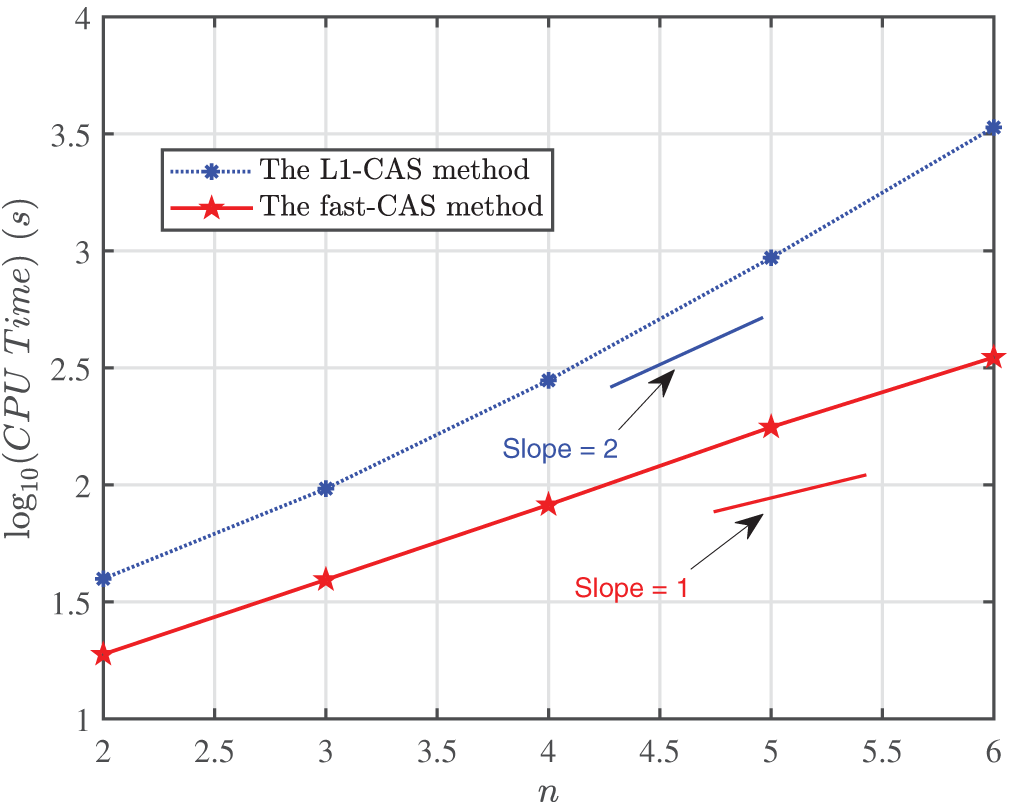
Figure 8: (Problem 3); Comparison of the fast-CAS and the L1-CAS method are presented for
This research paper makes two significant contributions to the existing literature. First, it introduces two novel methods, the L1-CAS and the fast-CAS, specifically designed for multiterm Caputo variable-order (CVO) fractional partial differential equations. Second, it combines these two methods with an interpolation technique, which has proven particularly effective for solving nonlinear multiterm CVO fractional partial differential equations. We have successfully derived the CAS wavelet operational matrix of variable-order fractional integration and applied it to boundary value problems. The implementation procedures of both methods are discussed in detail, and their pseudo codes are also provided. Numerical simulations are conducted to illustrate the theoretical results, and the findings are presented through both tabular and graphical formats. Separate truncation error estimates for temporal and spatial discretizations are given; however, a full space-time convergence analysis remains an open problem to be addressed in future work.
The results, including Figs. 1, 4, and 7, demonstrate that the fast-CAS method produces solutions in complete agreement with the exact solutions. Tables 1 to 5 and Figs. 2 and 5 show that the maximum absolute error decreases as the parameters
Although the CAS wavelet operational matrix method is accurate, it demands significant computational time, especially for large
Acknowledgement: Not applicable.
Funding Statement: This work was supported by the National Research Foundation of Korea (NRF) grant funded by the Korean government (MSIT) (NRF-2021R1A2C1011817) and the BK21 Program (Next Generation Education Program for Mathematical Sciences, 4299990414089) funded by the Ministry of Education (MOE, Republic of Korea).
Author Contributions: The authors confirm their contribution to the paper as follows: Junseo Lee: Formal analysis, software, methodology, data collection, visualization. Bongsoo Jang: Conceptualization, supervision, resources, funding acquisition. Umer Saeed: Conceptualization, formal analysis, methodology, validation. All authors reviewed the results and approved the final version of the manuscript.
Availability of Data and Materials: The datasets generated or analyzed during the current study are available from the corresponding author on reasonable request.
Ethics Approval: Not applicable.
Conflict of Interest: The authors declare no conflicts of interest to report regarding the present study.
References
1. Awati VB, Goravar A, Kumar M. Spectral and Haar wavelet collocation method for the solution of heat generation and viscous dissipation in micro-polar nanofluid for MHD stagnation point flow. Math Comput Simul. 2024;215:158–83. doi:10.1016/j.matcom.2023.07.031. [Google Scholar] [CrossRef]
2. Rabiei K, Razzaghi M. An approach to solve fractional optimal control problems via fractional-order Boubaker wavelets. J Vib Control. 2022;29(7–8):1806–19. doi:10.1177/10775463211070902. [Google Scholar] [CrossRef]
3. Agrawal K, Kumar R, Kumar S, Hadid S, Momani S. Bernoulli wavelet method for non-linear fractional Glucose–Insulin regulatory dynamical system. Chaos Soliton Fract. 2022;164(5):112632. doi:10.1016/j.chaos.2022.112632. [Google Scholar] [CrossRef]
4. Faheem M, Raza A, Khan A. Collocation methods based on Gegenbauer and Bernoulli wavelets for solving neutral delay differential equations. Math Comput Simul. 2021;180(26):72–92. doi:10.1016/j.matcom.2020.08.018. [Google Scholar] [CrossRef]
5. Saeed U. A method for solving Caputo-Hadamard fractional initial and boundary value problems. Math Methods Appl Sci. 2023;46(13):13907–21. doi:10.1002/mma.9297. [Google Scholar] [CrossRef]
6. Saeed U, Rehman M. Haar wavelet-quasilinearization technique for fractional nonlinear differential equations. Appl Math Comput. 2013;220(1):630–48. doi:10.1016/j.amc.2013.07.018. [Google Scholar] [CrossRef]
7. Saeed U, Idrees S, Javid K, Din Q. Krawtchouk wavelets method for solving Caputo and Caputo-Hadamard fractional differential equations. Math Methods Appl Sci. 2022;45(17):11331–54. doi:10.1002/mma.8452. [Google Scholar] [CrossRef]
8. Hedayati M, Ezzati R, Noeiaghdam S. New procedures of a fractional order model of novel coronavirus (COVID-19) outbreak via wavelets method. Axioms. 2021;10(2):122. doi:10.3390/axioms10020122. [Google Scholar] [CrossRef]
9. Hedayati M, Ezzati R. A new operational matrix method to solve nonlinear fractional differential equations. Nonlinear Eng. 2024;13(1):20220364. doi:10.1515/nleng-2022-0364. [Google Scholar] [CrossRef]
10. Khan NA, Altaf S, Khan NA, Ayaz M. Haar wavelet Arctic Puffin optimization method (HWAPOMapplication to logistic models with fractal-fractional Caputo-Fabrizio operator. Partial Differ Equ Appl Math. 2025;13(2):101114. doi:10.1016/j.padiff.2025.101114. [Google Scholar] [CrossRef]
11. Khan NA, Ali M, Ara A, Khan MI, Abdullaeva S, Waqas M. Optimizing pantograph fractional differential equations: a Haar wavelet operational matrix method Partial. Differ Equ App Math. 2024;11(7):100774. doi:10.1016/j.padiff.2024.100774. [Google Scholar] [CrossRef]
12. Nemati S, Lima PM, Torres DFM. Numerical solution of variable-order fractional differential equations using Bernoulli polynomials. Fractal Fract. 2021;5(4):219. doi:10.3390/fractalfract5040219. [Google Scholar] [CrossRef]
13. Chen YM, Wei YQ, Liu DY, Yu H. Numerical solution for a class of nonlinear variable order fractional differential equations with Legendre wavelets. Appl Math Lett. 2015;46(2):83–8. doi:10.1016/j.aml.2015.02.010. [Google Scholar] [CrossRef]
14. Kanwal A, Boulaaras S, Shafqat R, Taufeeq B, Rahman M. Explicit scheme for solving variable-order time-fractional initial boundary value problems. Sci Rep. 2024;14(1):5396. doi:10.1038/s41598-024-55943-4. [Google Scholar] [PubMed] [CrossRef]
15. Guo Y, Ye G. Existence and uniqueness of weak solutions to variable-order fractional Laplacian equations with variable exponents. J Funct Spaces. 2021;2021(3):6686213. doi:10.1155/2021/6686213. [Google Scholar] [CrossRef]
16. Tajadodi H. Variable-order Mittag-Leffler fractional operator and application to mobile-immobile advection-dispersion model. Alex Eng J. 2022;61(5):3719–28. doi:10.1016/j.aej.2021.09.007. [Google Scholar] [CrossRef]
17. Shen S, Liu F, Chen J, Turner I, Anh V. Numerical techniques for the variable order time fractional diffusion equation. Appl Math Comput. 2012;218(22):10861–70. doi:10.1016/j.amc.2012.04.047. [Google Scholar] [CrossRef]
18. Zhang JL, Fang ZW, Sun HW. Exponential-sum-approximation technique for variable-order time-fractional diffusion equations. J Appl Math Comput. 2021;68(1):323–47. doi:10.1007/s12190-021-01528-7. [Google Scholar] [CrossRef]
19. Zhang J, Fang ZW, Sun HW. Robust fast method for variable-order time-fractional diffusion equations without regularity assumptions of the true solutions. Appl Math Comput. 2022;430:127273. doi:10.1016/j.amc.2022.127273. [Google Scholar] [CrossRef]
20. Fang ZW, Sun HW, Wang H. A fast method for variable-order Caputo fractional derivative with applications to time-fractional diffusion equations. Comput Math Appl. 2020;80(5):1443–58. doi:10.1016/j.camwa.2020.07.009. [Google Scholar] [CrossRef]
21. Zhang L, Zhang GF. Fast algorithms for high-dimensional variable-order space-time fractional diffusion equations. Comput Appl Math. 2021;40(4):116. doi:10.1007/s40314-021-01496-5. [Google Scholar] [CrossRef]
22. Dehestani H, Ordokhani Y, Razzaghi M. A novel direct method based on the Lucas multiwavelet functions for variable-order fractional reaction-diffusion and subdiffusion equations. Numer Linear Algebra Appl. 2021;28(2):e2346. doi:10.1002/nla.2346. [Google Scholar] [CrossRef]
23. Heydari MH, Avazzadeh Z, Razzaghi M. Vieta-Lucas polynomials for the coupled nonlinear variable-order fractional Ginzburg-Landau equations. Appl Numer Math. 2021;165(2):442–58. doi:10.1016/j.apnum.2021.03.007. [Google Scholar] [CrossRef]
24. Hosseininia M, Heydari MH, Avazzadeh Z. A hybrid wavelet-meshless method for variable-order fractional regularized long-wave equation. Eng Anal Bound Elem. 2022;142(1):61–70. doi:10.1016/j.enganabound.2022.05.021; [Google Scholar] [CrossRef]
25. Jia J, Wang H, Zheng X. A fast algorithm for time-fractional diffusion equation with space-time-dependent variable order. Numer Algorithms. 2023;94(4):1705–30. doi:10.1007/s11075-023-01552-7. [Google Scholar] [CrossRef]
26. Dehestani H, Ordokhani Y, Razzaghi M. Pseudo-operational matrix method for the solution of variable-order fractional partial integro-differential equations. Eng Comput. 2021;37(3):1791–806. doi:10.1007/s00366-019-00912-z. [Google Scholar] [CrossRef]
27. Dehestani H, Ordokhani Y, Razzaghi M. Application of the modified operational matrices in multiterm variable-order time-fractional partial differential equations. Math Methods Appl Sci. 2019;42(18):7296–7313. doi:10.1002/mma.5840. [Google Scholar] [CrossRef]
28. Biswas C, Das S, Singh A, Altenbach H. Solution of variable-order partial integro-differential equation using Legendre wavelet approximation and operational matrices. Z Angew Math Mech. 2023;103(2):e202200222. doi:10.1002/zamm.202200222. [Google Scholar] [CrossRef]
29. Heydari MH, Cattani C, Hooshmandasl MR, Hariharan G. An optimization wavelet method for multi variable-order fractional differential equations. Fundam Inform. 2017;151(1–4):255–73. doi:10.3233/FI-2017-1491. [Google Scholar] [CrossRef]
30. Shah K, Naz H, Sarwar M, Abdeljawad T. On spectral numerical method for variable-order partial differential equations. AIMS Math. 2022;7(6):10422–38. doi:10.3934/math.2022581. [Google Scholar] [CrossRef]
31. Yousefi S, Banifatemi A. Numerical solution of Fredholm integral equations by using CAS wavelets. Appl Math Comput. 2006;183(1):458–63. doi:10.1016/j.amc.2006.05.081. [Google Scholar] [CrossRef]
32. Saeed U. CAS Picard method for fractional nonlinear differential equation. Appl Math Comput. 2017;307(1):102–12. doi:10.1016/j.amc.2017.02.044. [Google Scholar] [CrossRef]
33. Beylkin G, Monzón L. Approximation by exponential sums revisited. Appl Comput Harmon Anal. 2010;28(2):131–49. doi:10.1016/j.acha.2009.08.011. [Google Scholar] [CrossRef]
34. Yi H, Chen Y, Wang Y, Huang Y. Optimal convergence analysis of a linearized second-order BDF-PPIFE method for semi-linear parabolic interface problems. Appl Math Comput. 2023;438(3):127581. doi:10.1016/j.amc.2022.127581. [Google Scholar] [CrossRef]
35. Bellman RE, Kalaba RE. Quasilinearization and nonlinear boundary-value problems. New York, NY, USA: American Elsevier Publishing Company; 1965. doi:10.2307/3612757. [Google Scholar] [CrossRef]
36. Cherruault Y. Convergence of Adomian’s method. Math Comput Model. 1990;14:83–6. doi:10.1016/0895-7177(90)90152-D. [Google Scholar] [CrossRef]
37. Mittag-Leffler GM. Sur la nouvelle fonction Eα(x). Comptes Rendus de l′ Académie Des Sciences. 1903;137:554–8. [Google Scholar]
Cite This Article
 Copyright © 2025 The Author(s). Published by Tech Science Press.
This work is licensed under a Creative Commons Attribution 4.0 International License , which permits unrestricted use, distribution, and reproduction in any medium, provided the original work is properly cited.
 Downloads
 Citation Tools