
 Submit a Paper
 Propose a Special lssue
 Open Access
ARTICLE
A Novel Reduced Error Pruning Tree Forest with Time-Based Missing Data Imputation (REPTF-TMDI) for Traffic Flow Prediction
1 Department of Computer Engineering, Dokuz Eylul University, Izmir, 35390, Turkey
2 Independent Researcher, Izmir, 35140, Turkey
3 Graduate School of Natural and Applied Sciences, Dokuz Eylul University, Izmir, 35390, Turkey
4 Information Technologies Research and Application Center (DEBTAM), Dokuz Eylul University, Izmir, 35390, Turkey
* Corresponding Author: Derya Birant. Email:
Computer Modeling in Engineering & Sciences 2025, 144(2), 1677-1715. https://doi.org/10.32604/cmes.2025.069255
Received 18 June 2025; Accepted 12 August 2025; Issue published 31 August 2025
 View Full Text
 Download PDF
Abstract
Accurate traffic flow prediction (TFP) is vital for efficient and sustainable transportation management and the development of intelligent traffic systems. However, missing data in real-world traffic datasets poses a significant challenge to maintaining prediction precision. This study introduces REPTF-TMDI, a novel method that combines a Reduced Error Pruning Tree Forest (REPTree Forest) with a newly proposed Time-based Missing Data Imputation (TMDI) approach. The REPTree Forest, an ensemble learning approach, is tailored for time-related traffic data to enhance predictive accuracy and support the evolution of sustainable urban mobility solutions. Meanwhile, the TMDI approach exploits temporal patterns to estimate missing values reliably whenever empty fields are encountered. The proposed method was evaluated using hourly traffic flow data from a major U.S. roadway spanning 2012–2018, incorporating temporal features (e.g., hour, day, month, year, weekday), holiday indicator, and weather conditions (temperature, rain, snow, and cloud coverage). Experimental results demonstrated that the REPTF-TMDI method outperformed conventional imputation techniques across various missing data ratios by achieving an average 11.76% improvement in terms of correlation coefficient (R). Furthermore, REPTree Forest achieved improvements of 68.62% in RMSE and 70.52% in MAE compared to existing state-of-the-art models. These findings highlight the method’s ability to significantly boost traffic flow prediction accuracy, even in the presence of missing data, thereby contributing to the broader objectives of sustainable urban transportation systems.Keywords
Traffic flow prediction (TFP) [1] is important to facilitate the optimal functioning of modern traffic networks and to address the growing challenges posed by increasing traffic volumes. Having traffic flow information plays an important role in assisting transportation engineers in planning strategies to reduce the problem of traffic congestion and to advance the efficiency of traffic network operations. Another benefit of traffic flow information is that it helps users in orienting the travel routes, reducing travel times on the road. This information also aids in better managing traffic events, such as accidents or roadwork, by providing real-time insights. In order to support these efforts and build more sustainable urban transportation systems, traffic data is gathered from various sources, such as surveillance cameras, loop detectors, GPS-controlled equipment, and mobile applications.
Machine learning (ML) [2] methods have proven highly effective in traffic flow prediction, leveraging historical traffic data to identify underlying trends. These methods model the relationships among various factors, such as time of day, weather conditions, and special events, to generate accurate predictions of future traffic patterns. By analyzing these historical data points, ML algorithms can recognize subtle outlines that may be missed by traditional statistical methods, enabling more precise forecasting. The ability of ML techniques to continuously learn from new data also allows them to adapt to changing traffic behaviors and environmental factors over time. Consequently, transportation systems can better predict traffic distribution, improving management, route planning, and decision-making for engineers and road users.
Challenges in traffic flow prediction arise because traffic is affected by multiple complex factors, including environmental conditions, road types, and traffic incidents. Traffic flows change over time in a significant and non-linear manner, influenced by a variety of interrelated variables. In other words, there is a non-linear relationship among these factors, making it difficult to predict traffic flows accurately using traditional methods. The performance of ML models heavily depends on the availability of high-quality data, which is critical for training robust models. However, a common issue in real-world datasets is the problem of missing data, which can undermine the success of predictive models. Incomplete data may arise due to sensor malfunctions, communication errors, or gaps in data collection, further complicating accurate predictions. In spite of the recent advancements in traffic flow prediction, existing methods often struggle with missing data and fail to adapt to dynamic traffic patterns. Overcoming these data challenges is essential for achieving sustainable traffic management [3]. Our study seeks to bridge this gap by combining a novel time-based imputation technique with ensemble learning for more robust traffic flow predictions.
Missing data is a significant problem in machine learning studies. It is a widespread issue; for example, the absence of air/water quality sensor readings, unavailable values on vehicle track points, or the shortages in telecommunication signaling records. These gaps can significantly affect the performance of predictive models, especially when accurate and continuous data is essential. When missing data occurs, traditional methods often fail to achieve satisfactory precision. Simply removing records containing missing data could result in the loss of valuable information; therefore, methods to accurately interpolate missing data are required. Potent techniques are essential not only for maintaining data quality but also for ensuring the reliability of model predictions in the presence of information deficiencies [4].
Missing data imputation (MDI) is a procedure in machine learning that aims to fill in missing values in datasets. Traditional imputation techniques, such as mean/mode imputation or nearest neighbor imputation, rely on global patterns or simple heuristics to fill in missing values. Although these methods can be effective in some cases, they often fail to capture the underlying temporal or sequential patterns inherent in time-related data, such as traffic flow data. These methods may also struggle when the missing data occurs in a large chunk, or when the relationships between variables are complex and non-linear. As a result, traditional MDI methods can undermine the truthfulness of traffic flow predictions. To address these limitations, we propose a time-based missing data imputation (TMDI) approach that considers the temporal correlation between values at different timestamps. Unlike traditional methods, which rely solely on global or static patterns, the TMDI approach enables more accurate interpolation of missing values by focusing on the dynamic nature of temporal data [5]. The main idea behind our approach is that values with a shorter time distance are typically more similar than those with a larger time gap, thereby strengthening the imputation process.
While productive data imputation is essential for handling missing values, the predictive models themselves must also be robust enough to process the imputed data and generate precise traffic flow forecasts. The reduced error pruning tree (REPTree) [6] is a valuable machine learning algorithm, predominantly due to its error-based pruning strategy that enhances the generalization ability of decision trees. A key advantage of REPTree is its use of a validation set to eliminate unnecessary branches, allowing the machine-learning model to focus on the most relevant patterns—an especially useful trait when working with noisy datasets. REPTree supports both categorical and numerical attributes and has demonstrated success across various domains, including animal science, environmental modeling, healthcare, and education. Its simplicity and interpretability make it a practical solution for many real-world applications. Its functionality can be significantly developed when incorporated into ensemble frameworks using bootstrap aggregating (Bagging) [7]. Building on these strengths, we present REPTree Forest, an ensemble approach that integrates multiple REPTrees to increase predictive accuracy. This collective learning strategy allows the model to better capture complex data variations and deliver more reliable traffic flow predictions in a sustainable system. Beyond technical advancements, the broader societal impacts of our study are equally significant.
By proposing a machine learning-based approach (REPTF-TMDI), we aim to improve the prediction of traffic volume using temporal and environmental features such as day, month, year, hour, weekday, holiday status, temperature, rainfall, snowfall, cloud coverage, and weather conditions. This study also highlights the positive sustainability implications of improving traffic flow prediction accuracy, contributing to the goals of “Sustainable Cities and Communities” (Goal 11) and “Life on Land” (Goal 15) as outlined by the universal Sustainable Development Goals (SDGs). Accurate traffic forecasting allows urban planners and authorities to optimize traffic management, minimize congestion, and lower vehicle emissions, thereby supporting safer, more efficient, and sustainable cities. Additionally, enriched traffic flow supports emergency response planning and minimizes the adverse environmental impacts of transportation systems. As a result, it helps mitigate land degradation, reduce urban sprawl, and prevent unnecessary ecological disruption. By providing a data-driven foundation for informed and proactive planning, the proposed model contributes meaningfully to the preservation of ecosystems and the sustainable use of land resources.
The major contributions of this study are summarized as follows:
• Presentation of REPTree Forest (REPTF): This study describes REPTree Forest as an ensemble learning model that aggregates multiple reduced error pruning trees to enhance generalization, reduce variance, and improve predictive accuracy for traffic flow prediction. The REPTree Forest benefits from the individual strengths of decision tree models, offering fast training, high interpretability, and reliable precision, making it practical for real-world applications.
• Proposal of time-based missing data imputation (TMDI): TMDI is introduced as a new missing data imputation method, specifically for time-related traffic datasets. It utilizes temporal proximity between timestamps to reconstruct missing values more realistically, overcoming the limitations of traditional imputation techniques such as mean/mode and user-based imputations that often neglect temporal continuity.
• Introduction of hybrid REPTF-TMDI method: The study uniquely integrates the REPTree Forest and TMDI into a hybrid method as REPTF-TMDI, providing a robust solution for traffic flow prediction even in the presence of substantial missing data. This hybrid method is introduced for the first time in the literature.
• Extensive experimental evaluation: A thorough evaluation of the REPTF-TMDI method was conducted using the metro interstate traffic volume (MITV) dataset, covering 48,204 hourly records from 2012 to 2018. Various missing data rates (5% to 40%) were simulated, and performance was compared against conventional imputation techniques (mean/mode and user-based imputation). The REPTF-TMDI method outperformed these previous techniques by achieving an average 11.76% improvement in terms of correlation coefficient (R). Furthermore, four supplementary datasets from diverse regions confirmed the method’s consistent performance.
• Feature importance analysis for traffic flow prediction: A detailed feature importance analysis using mutual information was performed. Results reveal that the hour of the day, temperature, and weekday were the most influential features on traffic flow, while holiday and snow had minimal impact. This finding boosts understanding of which temporal and environmental factors most strongly affect traffic dynamics.
• Performance improvements and sustainability implications: Experimental results showed that REPTree Forest achieved 68.62% improvement in RMSE and 70.52% improvement in MAE when compared with 14 state-of-the-art studies. By enhancing prediction accuracy, the proposed method also contributes to advancing sustainable urban transportation systems.
• The remainder of this paper is organized as follows. Section 2 reviews related work in the field. In Section 3, a detailed explanation of the proposed method is provided. Section 4 outlines the experimental setup, covering the dataset, preprocessing steps, REPTF-TMDI model hyperparameters, and evaluation metrics. Section 5 presents detailed experimental results from various perspectives, including the effects of missing data rates and the final REPTree structure. Section 6 discusses the findings under different conditions, such as comparisons with recent studies and alternative methods, supported by sensitivity analyses and an assessment of generalizability. Finally, Section 7 concludes the paper and suggests directions for future research.
The related works [8–12] in traffic flow prediction cover a wide variety of regions, tasks, methodologies, and performance metrics. The studies [13–17] have addressed unique challenges posed by different geographic contexts, data availability, and prediction goals. We investigated related works [18–22], which provide valuable insights into the emergence of robust models for traffic flow forecasting. These efforts contribute to a better understanding of the methods and approaches used in predicting traffic flow under diverse conditions [23–27].
Traffic Traffic flow prediction has been studied in a diverse range of regions, such as Southern Africa [28], Spain [29], China [30], and the United States [31]. For instance, in China [32], various studies focused on predicting traffic flow in urban areas with dense traffic and frequent congestion, while in the USA [33], the focus was on optimizing traffic flow for highways and managing the unpredictability of urban commuting. Each region presents its own set of challenges due to varying traffic conditions, sensor infrastructure, and environmental factors [34,35]. Developing sustainable traffic management strategies in these diverse contexts required truthful and adaptable prediction models.
Some of the studies focused on regression tasks, such as [19,33], while others focused on classification tasks [10,30,35]. Others were centered on time-series prediction tasks like [8,15,21,31,32]. Regression tasks were typically aimed at predicting continuous traffic flow values, while classification tasks categorized traffic conditions into different classes, such as congestion or free flow. Time-series tasks, on the other hand, involved predicting future traffic flow based on temporal patterns and trends. For instance, time-series models like long short-term memory (LSTM) and autoregressive integrated moving average (ARIMA) were commonly used for modeling traffic flow over time, while regression models such as logistic regression (LR) and support vector regression (SVR) were often used for forecasting specific traffic flow values.
Some studies utilized traditional machine learning methods such as support vector machine (SVM) [35], decision tree (DT) [14], k-nearest neighbors (KNN) [17], random forest (RF) [11], and ElasticNet (EN) [25]. Others used deep learning methods such as LSTM [13,23], convolutional neural networks (CNN) [29], gated recurrent units (GRU) [15], and bidirectional LSTM (BILSTM) [16]. These methods vary in complexity and the type of patterns they can capture, with traditional models generally excelling in simpler, less nonlinear data, while deep learning models are often more adept at handling complex, high-dimensional datasets with temporal dependencies.
In sample studies, the root mean square error (RMSE) [21,33], mean absolute error (MAE) [27], and mean absolute percentage error (MAPE) [12,31] measures were used to evaluate the models, as they provide insight into the magnitude and percentage of prediction errors in regression and time-series forecasting. Additional regression evaluation metrics include the mean squared error (MSE) such as [28], symmetric mean absolute percentage error (SMAPE) [11], explained variance (EV) [27], and the correlation coefficient (R) [19,32]. Some studies also used absolute error (AE) [34] and the equilibrium coefficient (EC) [32] for error analysis and model robustness assessment. For classification tasks, metrics such as accuracy (ACC) [35], precision (P) [10], recall (RC) [35], and F1-score [30] were commonly used to evaluate classification outputs. In some cases, specificity [35] and the accuracy ratio (A) [19] were also applied to provide a more comprehensive view of model capability in traffic condition classification.
The summary of studies for traffic flow prediction reviewed in this work is presented in Table 1. Each row in the table corresponds to a specific study and provides detailed information across several key columns, including ref (reference number), year (publication year), region (geographic location of the study), methods (prediction techniques used), C, R, and T (which indicate whether the study involves a classification, regression, or time-series prediction task, respectively—checked if applicable), period (the time frame during which data was collected), data (the nature or source of dataset used), and performance metrics (the evaluation measures reported in each study).
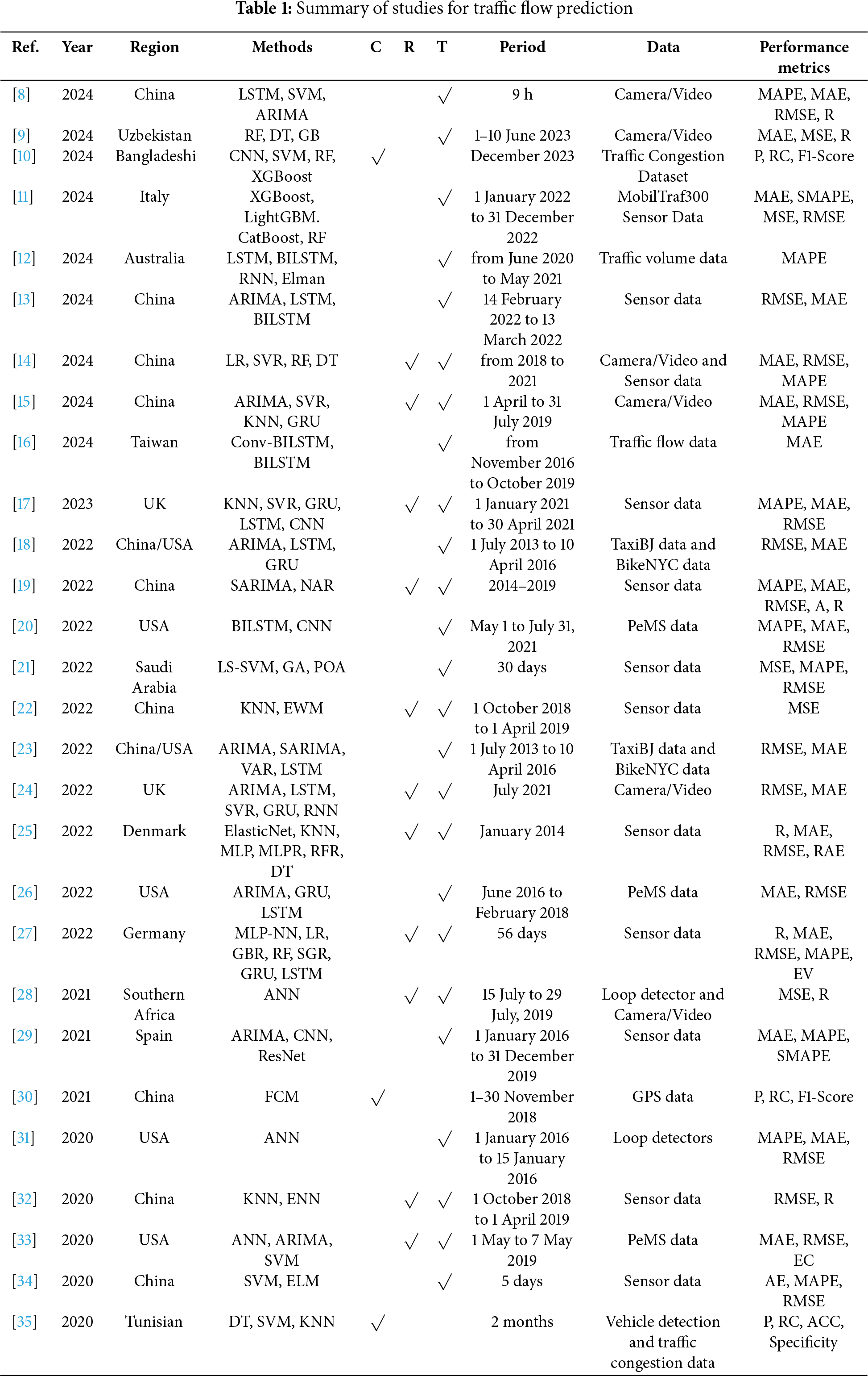
Table 1 summarized recent studies focused on traffic flow prediction to represent the variety of methods, datasets, and performance metrics applied within this domain. Beyond traffic-specific studies, related research has demonstrated the expanding role of data-driven modeling techniques across various disciplines in handling complex prediction tasks. For instance, recent works have successfully integrated physics-based simulations with AutoML to predict material behavior from microscale parameters [36], while transformer-based deep learning models have shown high accuracy in classifying railway defects from ultrasonic image data [37]. These studies, although outside the immediate scope of traffic flow prediction, exemplify innovative approaches in intelligent modeling that could also inspire future developments in traffic-related applications.
In parallel with these broader trends, recent literature has focused on utilizing tree ensemble methods with time-aware or local imputation strategies for handling missing temporal data. For example, a detailed review of imputation techniques tailored for traffic datasets in [38] to emphasize the importance of leveraging temporal correlations between neighboring detectors. Their study benchmarked several methods, including tree-based approaches, under varying missing patterns and confirmed the superiority of models that incorporate temporal structure. Similarly, a machine learning-based method was proposed in [39] for imputing missing air quality data and its performance was compared with an ensemble of extremely randomized trees. Their findings indicate the competitive nature of ensemble tree models in time-aware imputation tasks, particularly when augmented with temporal features.
These recent studies underscore the relevance of combining ensemble learning with temporal imputation in spatiotemporal contexts, i.e., a direction in which our work also contributes by introducing the hybrid REPTF-TMDI method. The potency of the REPTree classifier has been demonstrated in several studies [40–44], where it has been compared with widely used methods such as SVM, KNN, artificial neural networks (ANN), and naive Bayes (NB). In [40], REPTree had the highest accuracy compared to KNN and NB techniques in predicting student academic performance. This highlights REPTree’s strength to enhance predictive accuracy in educational applications. In [41], REPTree consistently achieved higher accuracy than other machine-learning algorithms across the different sizes of the Internet of Things data.
Alongside models like DT, ANN, NB, and RandomTree, REPTree was noted for its stable and effective behavior, achieving better overall results compared to alternative approaches [42]. In the same study, it was stated that REPTree is a fast decision tree algorithm that constructs a regression/decision tree using a selection mechanism when splitting nodes and prunes the tree using a particular technique to simplify it. Further evidence of REPTree’s robustness can be found in [43], where it emerged as the most accurate classifier in a study focused on the prediction of structural properties in halide perovskite materials. In [44], REPTree once again had the best performance in predicting nitrate concentration in different type of watersheds. These results, derived from diverse application areas, reinforce REPTree’s strong generalization ability and justify its selection as a key model.
Beyond its strong predictive accomplishment, REPTree has also been recognized for several practical advantages that make it a favorable choice in diverse machine learning applications. As highlighted in [45], REPTree, as a fast decision tree learner, demonstrated better performance than LR and MLP in learning artifacts in limited-angle tomography. In [46], REPTree was shown to deliver accurate results across various algorithms in forecasting long-series daily reference evapotranspiration. Moreover, in [47], REPtree performed well compared to other machine learning algorithms such as M5P, ANN, fuzzy logic, and MLR investigated for modelling of streamflow.
One of the key operational strengths of REPTree lies in its rapid model training capabilities as discussed in [48]. It consistently demonstrated the shortest model-building times compared to other classifiers, emphasizing its efficiency in computational resource usage. Additionally, interpretability is another critical aspect where REPTree excels. In [49], REPTree was identified as one of the top-performing algorithms in terms of model transparency and ease of interpretation, which is especially important in decision-making scenarios where understanding the reasoning behind predictions is crucial.
Different from the studies aforementioned, our research employs an ensemble approach, REPTree Forest, which leverages the strengths of individual REPTree classifiers while developing overall prediction robustness through ensemble learning. While prior studies have primarily focused on the standalone execution and advantages of REPTree, the REPTree Forest structure provides an important perspective by combining multiple REPTree models to improve generalization and reduce variance.
In addition to the ensemble strategy, this study also introduces a time-based missing data imputation (TMDI) approach. Unlike conventional imputation methods, TMDI considers the temporal patterns and continuity in traffic data, which allows for a more realistic reconstruction of missing values. Together, these contributions form the hybrid REPTF-TMDI methodology, specifically designed to enhance traffic flow prediction while supporting sustainability goals in urban transportation systems, thereby distinguishing this study from existing REPTree applications in the literature.
This section outlines the proposed REPTF-TMDI method and its application for traffic flow prediction. By integrating TMDI for intelligent data completion and the REPTree Forest ensemble for prediction, the REPTF-TMDI method offers a robust solution to the dual challenges of missing data and valid traffic forecasting, while also contributing to the advancement of sustainable mobility initiatives.
A general overview of the proposed approach is represented in Fig. 1. A comprehensive dataset contains hourly traffic flow, weather conditions, and temporal variables collected from a roadway within a particular period. The traffic data reflect real-world patterns, while the weather data encompasses a variety of environmental conditions, including rain, snow, clouds, drizzle, thunderstorms, mist, smoke, and clear skies. Temporal features—such as hour, day, month, year, weekday, and holiday indicators—are incorporated to enrich the contextual understanding of traffic behavior over time. The raw data, stored in a centralized repository, usually exhibits common real-world issues such as missing values, which could arise from various factors like sensor errors, communication breakdowns, or other unforeseen circumstances. To address this, we introduce a novel time-based missing data imputation (TMDI) method. Unlike traditional statistical imputations, TMDI is mainly designed for temporal datasets. It employs temporal dependencies and recurring traffic patterns across various time periods to estimate missing entries. This approach enables a contextually informed reconstruction of incomplete records, resulting in a cleaner and more reliable dataset for subsequent analysis.
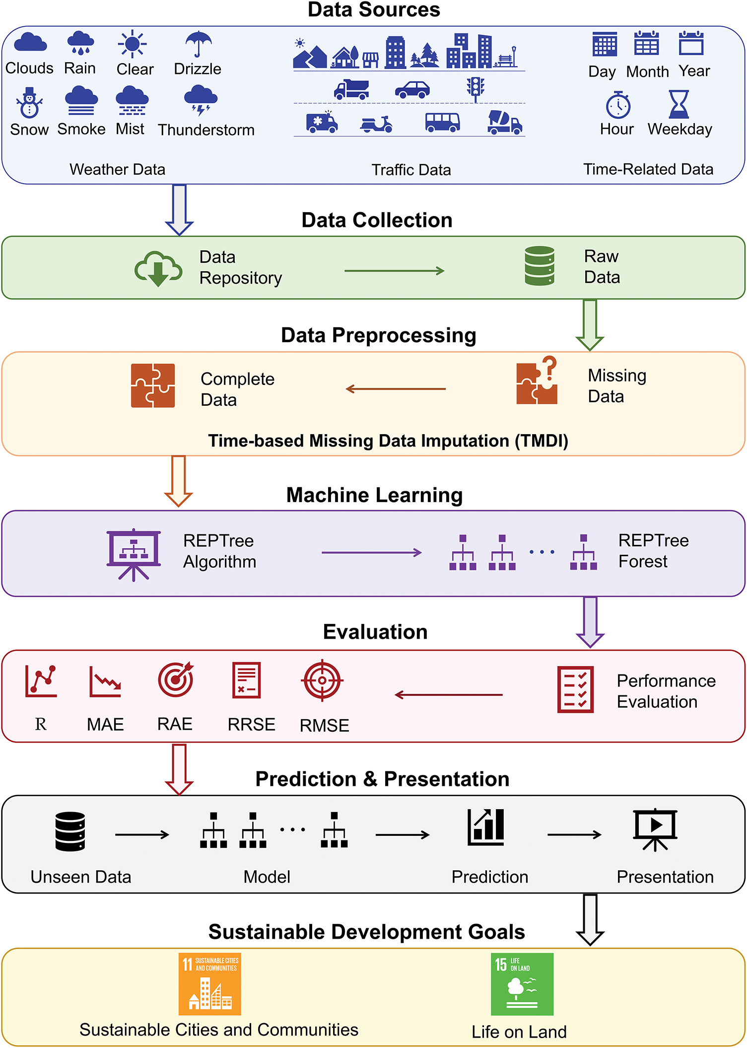
Figure 1: General overview of the proposed REPTF-TMDI method
After imputation, the processed dataset is used to train a predictive model based on the REPTree Forest algorithm. REPTree is a fast decision tree learner that builds models using a node splitting criterion and then prunes them through reduced-error pruning to prevent overfitting. Its efficiency and interpretability make it particularly well-suited for traffic flow prediction. By combining multiple REPTree models into an ensemble, the REPTF-TMDI method takes advantage of model diversity to refine generalization and pre-diction accuracy, especially for time-varying and complex traffic flow patterns. The ensemble approach reduces biases of individual models and harnesses the complementary strengths of the base learners. To thoroughly assess model operation, the algorithm uses various evaluation metrics, including the R, MAE, RAE, RRSE, and RMSE. These metrics capture both the absolute and relative predictive accuracy of the model, as well as its ability to preserve temporal trends in the data. Lastly, the trained REPTree Forest model was deployed to predict traffic flow on unseen data. The predictive results are then presented through visualizations, reports, or user interfaces that facilitate interpretation and decision-making. The predictions can play a significant role in many different scenarios in a decision support system that helps to enhance transportation efficiency, enable smart infrastructure planning, improve emergency response times, and promote data-driven urban development. In this respect, this study meets the objectives of “Sustainable Cities and Communities” and “Life on Land”, involving in Sustainable Development Goals.
3.2 Description of Methodologies
3.2.1 Time-Based Missing Data Imputation (TMDI)
To address the issue of missing values in temporal datasets, we propose a method called time-based missing data imputation (TMDI). The key idea behind TMDI is to estimate missing values using the most recent available data points that share the same/nearest day and time context. Missing data is filled in by considering the closest previous and/or subsequent data by day and time from the rest of the values. In other words, TMDI uses the observed data of adjacent points to estimate missing data.
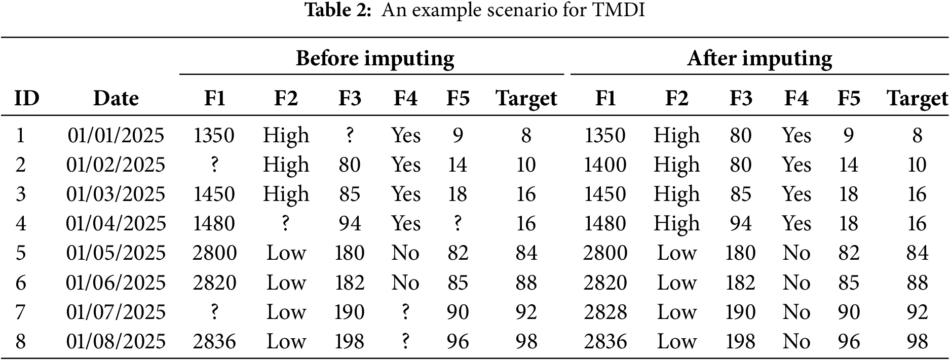
TMDI operates by scanning through each instance in the dataset and identifying missing values. For each missing entry, the algorithm searches backward and/or forward in time to find the closest previous and/or subsequent timestamps with a valid observation for the same feature. In cases where only one adjacent value is available, the missing entry is filled using this reference. In cases where multiple adjacent values are available, TMDI considers both forward and backward neighbors. If the value of the target attribute of the current record is equal to the corresponding target value of its neighbor record, the missing entry is filled using this reference. In this way, the method preserves the temporal consistency of the data and is especially efficacious in scenarios where traffic patterns are repetitive across similar times and days. In other words, priority is always given to the nearest valid entry, confirming that the imputation reflects immediate past behavior rather than long-term trends. If target values are different and the feature type is numerical, two adjacent values are averaged to fill an entry. If the feature type is nominal, the previous value is repeated.
Formally, let the dataset be represented as a matrix
Table 2 illustrates an example scenario at eight consecutive timestamps involving five sensors’ readings, labeled F1 to F5, along with a target column representing traffic volume. The data is organized as a matrix where each row denotes a specific timestamp and each column stands for a sensor reading or the target value. In this example, several values are missing: specifically, F3 at timestamp 1 (
Reduced error pruning tree (REPTree) is an efficient and fast decision tree learner that supports both classification and regression tasks. It is designed to construct interpretable trees while maintaining generalization through a pruning strategy. In the context of regression, which is the focus of this study, REPTree uses variance reduction to determine the optimal split at each node. Given a dataset in matrix format
where
where
Once the tree has been fully grown, REPTree applies a reduced-error pruning strategy to mitigate overfitting and optimize generalization. This method evaluates each subtree using a separate pruning set, typically a reserved subset of the training data used for evaluation. Principally, let
This pruning strategy follows a greedy approach, systematically replacing subtrees with simpler leaf nodes whenever doing so does not degrade delivery on the validation set. By eliminating branches that fail to contribute meaningful predictive gain, REPTree produces more compact models that generalize better to unseen data and are less prone to overfitting on the noise in the training set.
To boost predictive achievement, our proposed REPTF-TMDI method constructs an ensemble of REPTree regressors using the imputed dataset
where
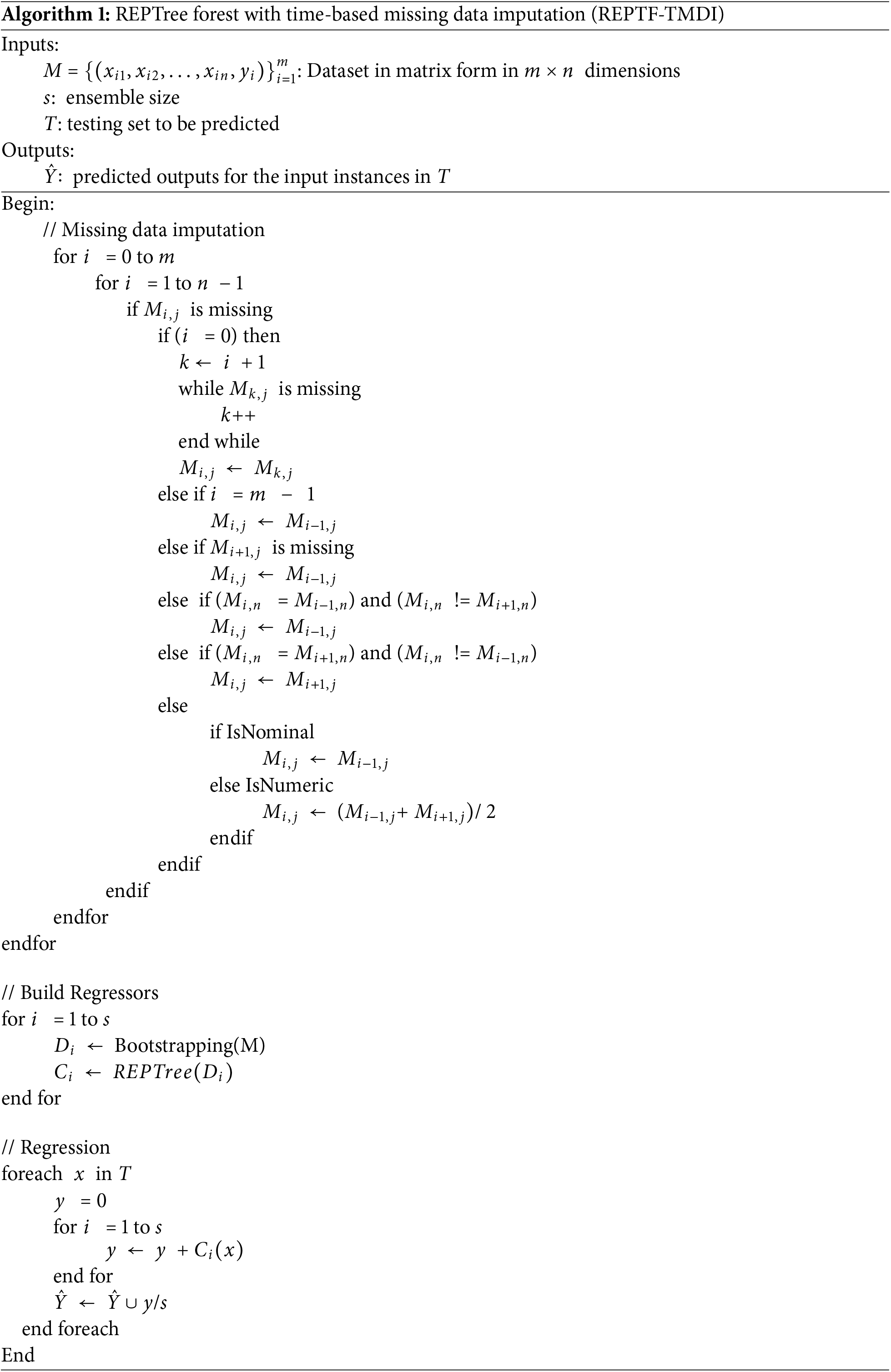
Algorithm 1 combines time-based missing data imputation (TMDI) with an ensemble of regression models to improve predictions, particularly in tasks such as traffic flow forecasting. The dataset
This resampling process contributes to diversity among the training subsets, enabling the ensemble to capture a broader range of data patterns and thereby upgrading its predictive ability. Each bootstrapped subset
This section can be divided by subheadings that provide a precise and concise description of the dataset and its preprocessing stage, as well as the details of experimental studies.
For the investigation of our proposed approach, REPTF-TMDI, this section describes the dataset used in the experimental study. The metro interstate traffic volume (MITV) dataset [50], obtained from the UCI Machine Learning Repository, contains 48,204 hourly records collected between 2012 and 2018. It records the westbound traffic volume on Interstate 94 (I-94), collected from the Minnesota Department of Transportation’s ATR Station 301, which is located approximately midway between the cities of Minneapolis and St. Paul, in the state of Minnesota, USA. The dataset comprises 12 features, including weather conditions and holiday indicators, which are critical external factors impacting traffic flow. As a multivariate, sequential, and time-related data designed for regression tasks, MITV provides a suitable and realistic environment to evaluate the temporal modeling and imputation capabilities of the REPTF-TMDI method.
Fig. 2 presents a segment of Interstate 94 (I-94) as it passes through the Minneapolis–St. Paul metropolitan area in the state of Minnesota, USA. The map depicts the west-bound direction of I-94, which serves as a major transportation route connecting key locations such as Minneapolis, St. Paul, Coon Rapids, St. Cloud, and Sauk Centre. The traffic volume data used in this study was collected near the midpoint of this route, specifically at the Minnesota Department of Transportation (MnDOT) automatic traffic recorder (ATR) station 301. This station is strategically located to capture representative traffic flow patterns between these two urban centers, making it a suitable location for studying related variables on interstate traffic volume and contributing to sustainable transportation systems.
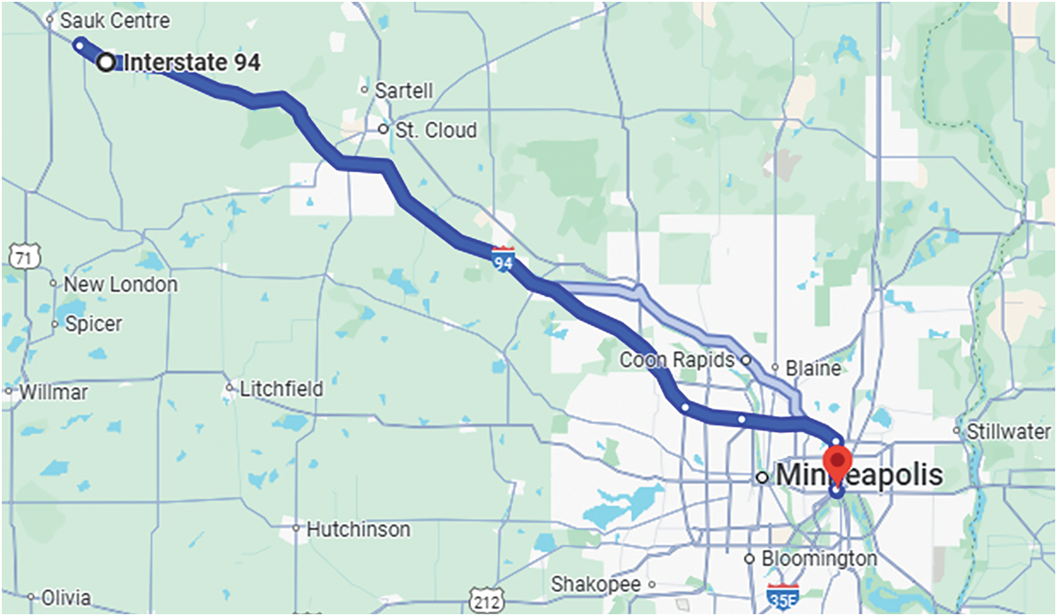
Figure 2: Google Maps view showing the location of ATR station 301, where the MITV dataset traffic data was collected
Table 3 outlines the features in the MITV dataset, grouped into four main categories, including time-related, basic, weather-related, and traffic-specific attributes. The time-related features—day, month, year, hour, and weekday—provide essential temporal context for each observation, enabling the analysis of daily, seasonal, and long-term trends. The basic feature, holiday, indicates whether the record falls on a public holiday, which can significantly impact traffic flow. Weather-related features include temperature (in Kelvin), rain_1h and snow_1h (in millimeters), clouds_all (as a percentage of cloud cover), as well as general and detailed weather conditions such as clear, rain, or overcast clouds. These features capture the environmental factors that may influence driving behavior and traffic volume. Lastly, the traffic_volume feature represents the number of vehicles passing through ATR station 301 during each recorded hour and serves as the target variable for prediction. This diverse set of features supports reliable modeling of traffic patterns under varying temporal and meteorological conditions.
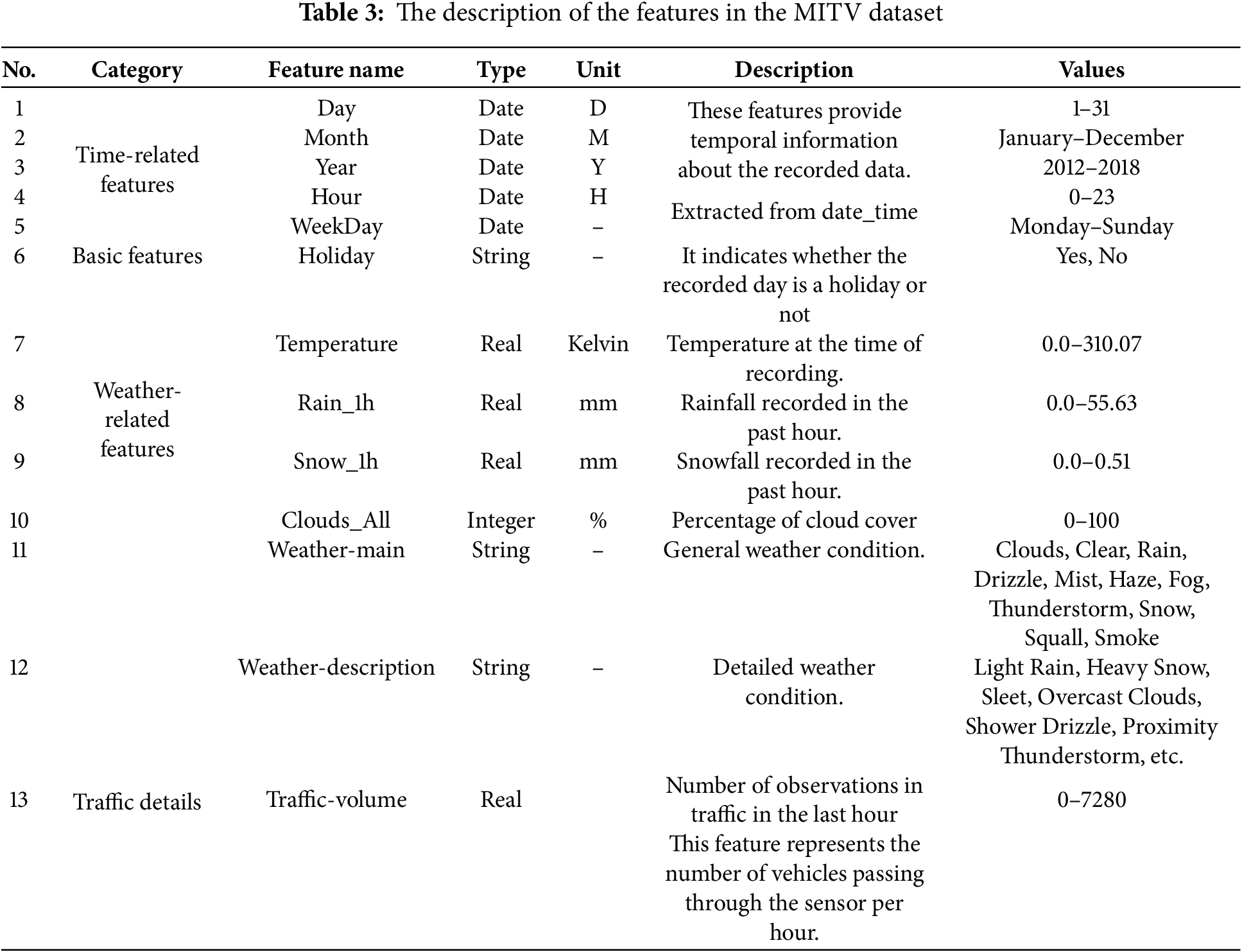
Table 4 presents a partial view of the MITV dataset, indicating hourly traffic volume observations along with corresponding features. Each row represents a specific hour of data collection, including details such as holiday status, temperature, rainfall, and snowfall in the past hour, cloud coverage, and both general and detailed weather conditions. The date_time field provides the exact timestamp of each observation, while the traffic_volume column showcases the number of vehicles recorded during that hour. For example, on 9 September 2016, at 6:00 AM, the weather was characterized by moderate rain, with a temperature of 289.88 K, 0.43 mm of rainfall, no snowfall, and cloud coverage at 90%. The recorded traffic volume at that time was 5411 vehicles. In contrast, during a holiday on 7 September 2015, at 7:00 AM, the sky was clear, with a temperature of 291.85 K, no precipitation, minimal cloud coverage, and a significantly lower traffic volume of 1658 vehicles—possibly reflecting reduced commuting activity on holidays. Another interesting case is 9 September 2016, at 5:00 AM, which saw a proximity thunderstorm with no rain or snow, a temperature of 289.87 K, and only 1% cloud coverage, yet the traffic volume sharply increased to 2763 vehicles, potentially showcasing the start of morning traffic buildup despite adverse conditions. Overall, the table illustrates how traffic volume fluctuates to form a sample context for analyzing traffic behaviors under varying environmental conditions.
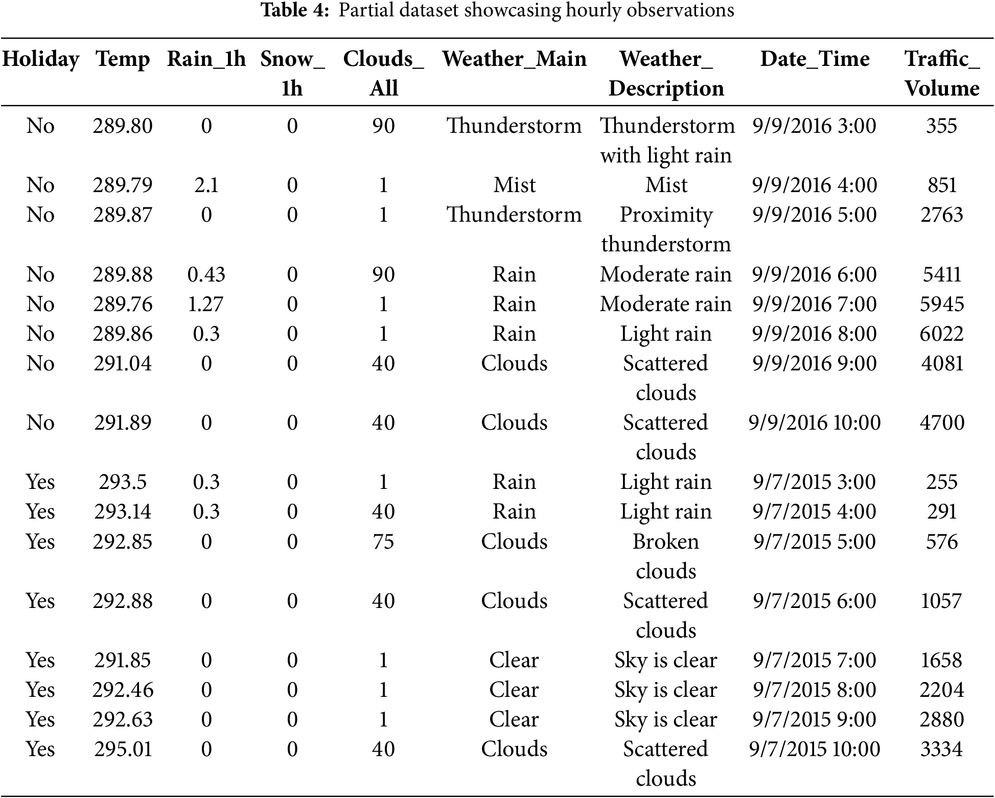
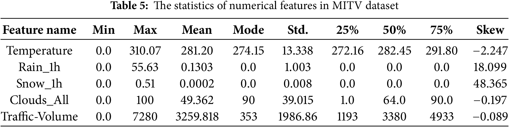
Table 5 provides a statistical summary of the numerical features in the MITV dataset, which includes temperature, rainfall, snowfall, cloud coverage, and traffic volume. For each feature, key statistics such as the minimum, maximum, mean, mode, standard deviation (std.), as well as the 25th, 50th (median), and 75th percentiles, are provided, along with the skewness (skew) value. For example, the temperature feature ranges from 0.0 to 310.07 K, with a mean value of 281.20 K and a standard deviation of 13.34. The rain_1h feature shows significant variation, with a maximum value of 55.63 mm but a mean of only 0.1303 mm, representing the occasional extreme weather events. The snow_1h feature has a very low mean of 0.0002 mm, with many instances showing zero snowfall. Cloud coverage varies from 0% to 100%, with a mean of 49.36% and a mode of 90%, demonstrating that overcast skies are common in the dataset. The traffic_volume feature shows a wide range of values, from 0 to 7280 vehicles, with a mean of 3259.82 vehicles per hour and a standard deviation of 1986.86, illustrating the high variability in traffic flow. The skewness values for most features, such as traffic volume and cloud coverage, confirm slight asymmetry in their distributions.
4.2.1 Feature Extraction and Transformation
Before model development, the MITV dataset underwent several preprocessing steps, including feature extraction and feature transformation, to enhance feature utility and ensure consistency across all observations. As part of feature extraction, the original date_time attribute—recording the timestamp of each traffic volume entry—was decomposed into multiple time-related features as day, month, year, hour, and weekday. This allowed for more detailed temporal analysis and enabled the model to capture recurring patterns tied to specific time intervals. In the feature transformation phase, the holiday attribute, which initially included specific holiday names (e.g., “Christmas Day”), was converted into a binary format with “yes” indicating a holiday and “no” otherwise. To ensure consistency, all 24-h records corresponding to a holiday were updated to reflect the “yes” value, rather than marking only the first hour. These extraction and transformation efforts improved the structure and reliability of the dataset, enabling more valid traffic pattern modeling.
4.2.2 Visual Explorations of Feature-Target Relationships
To gain an initial understanding of how traffic volume varies with different features, Fig. 3 presents boxplots that visually compare traffic volume distributions across various categorical and temporal dimensions. Fig. 3a shows the influence of weather conditions on traffic volume. Clear and cloudy weather conditions are associated with higher traffic volumes, while adverse conditions such as squalls and thunderstorms correspond to slightly lower median volumes. In Fig. 3b, traffic volume across years remains fairly stable without drastic fluctuations, suggesting consistency in travel demand over the study period. Fig. 3c explores monthly variations, showing higher traffic volumes during June and lower volumes during December, likely reflecting seasonal travel behaviors. Fig. 3d highlights weekly patterns, where weekdays exhibit higher median traffic volumes compared to weekends, aligning with typical workweek commuting patterns. Fig. 3e reveals distinct hourly trends, with traffic volume peaking during the morning (7:00–9:00) and the evening (16:00–18:00) rush hours, and lower traffic observed overnight.
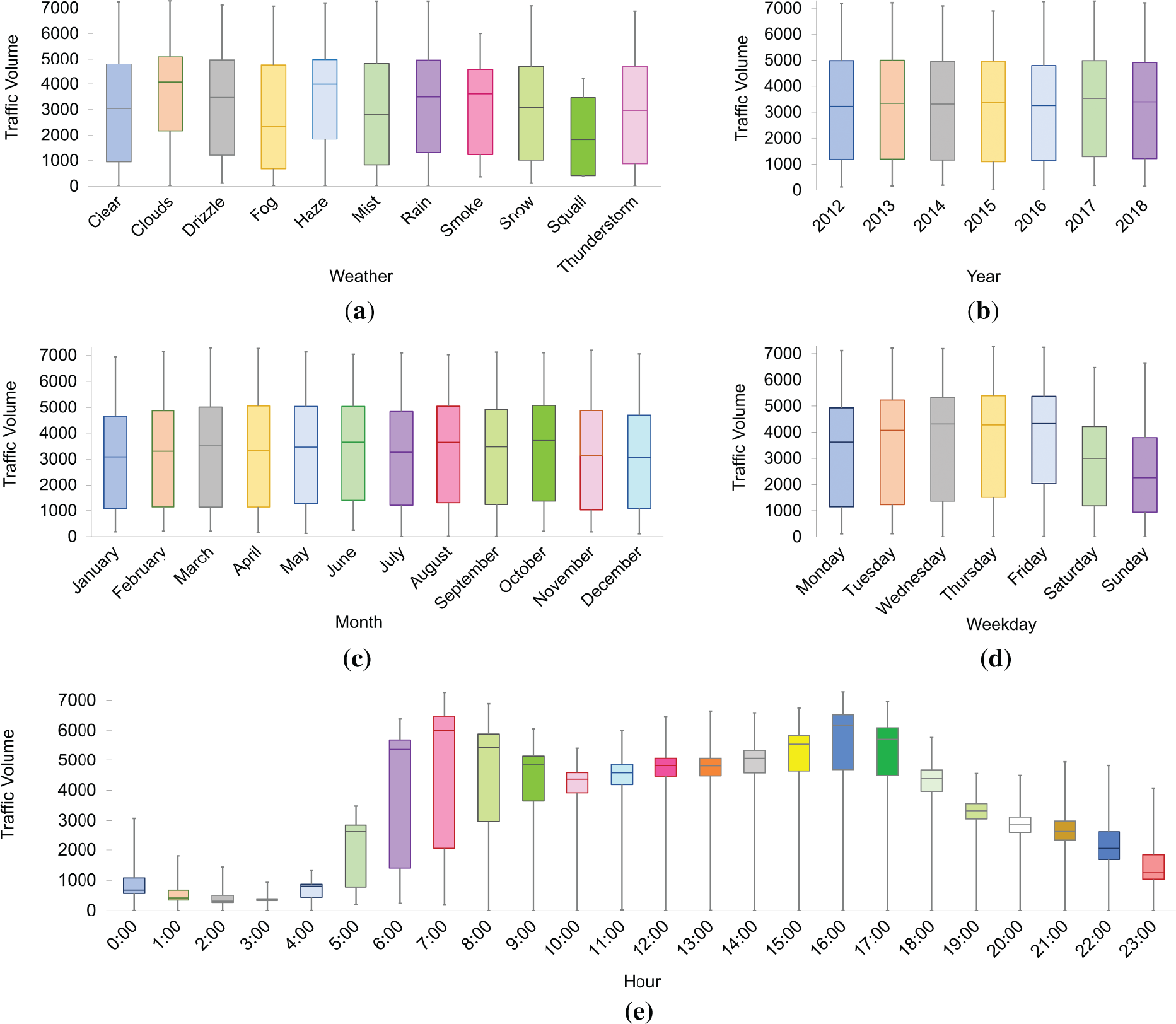
Figure 3: Boxplots illustrating the distribution of traffic volume across different feature categories: (a) weather conditions, (b) years, (c) months, (d) weekdays, and (e) hours of the day
To further complement and validate the observations, Fig. 4 presents line plots depicting the average traffic volume trends across the same temporal dimensions. Fig. 4a shows the yearly variation in average traffic volume. While the overall trend remains relatively stable, a notable dip in 2016, followed by a sharp increase in 2017, suggests external factors, such as infrastructural developments or policy changes, may have influenced traffic patterns during this period. Fig. 4b captures weekly trends, revealing that traffic volume gradually increases from Monday to Friday, peaking on Friday before significantly dropping over the weekend. This aligns with typical workweek travel behavior, where commuting is more intensive on weekdays compared to weekends. Monthly trends are depicted in Fig. 4c, where traffic volumes rise from January, peak in mid-year (June–July), and then decline in August and December, likely influenced by vacation and holiday seasons. Fig. 4d illustrates hourly traffic patterns, highlighting two distinct peaks corresponding to morning and evening commuting hours and minimal traffic volume during late-night and early-morning periods.
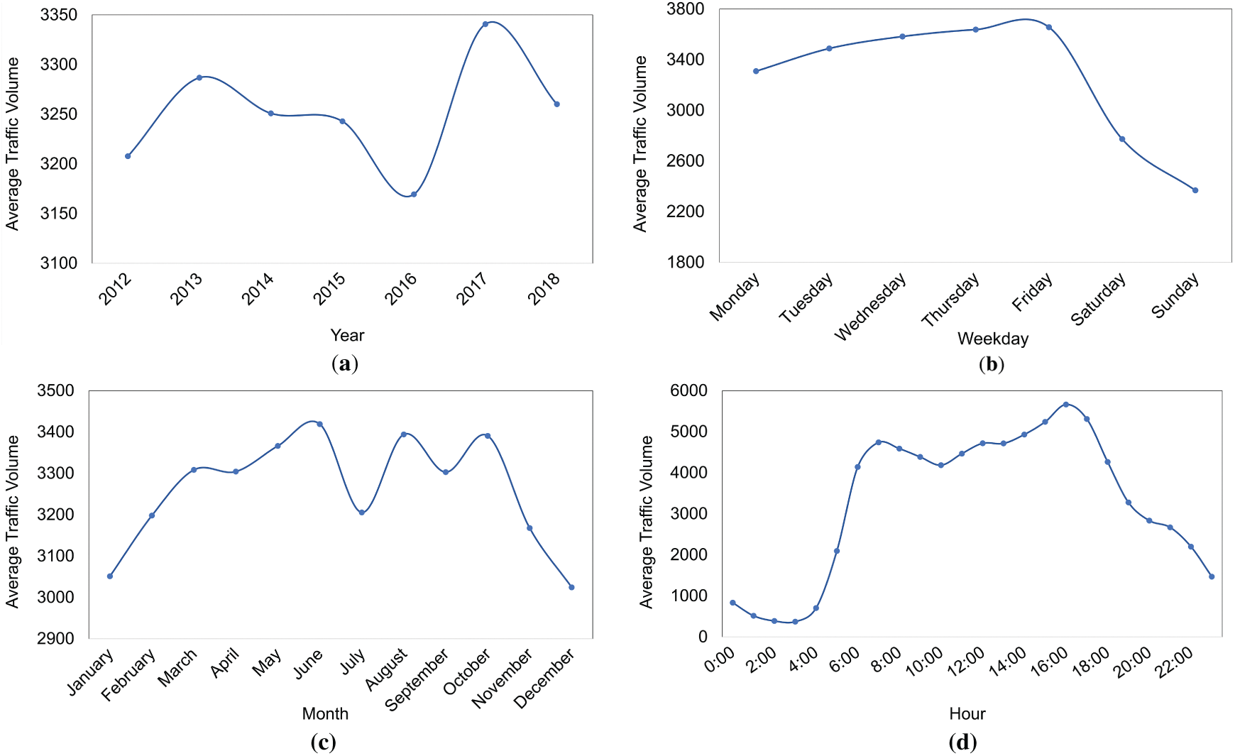
Figure 4: Line plots showing the average traffic volume trends by (a) year, (b) weekday, (c) month, and (d) hour of the day
To extend the exploration, Fig. 5 examines how traffic volume varies between holidays and non-holidays. The bar chart clearly shows that the average traffic volume is significantly lower on holidays compared to regular days. This is consistent with expectations, as holidays often result in reduced commuting and work-related travel. The drop in traffic volume on holidays further reinforces the role of temporal and contextual variables in influencing traffic behavior. Including holiday indicators in predictive models can therefore strengthen their ability to capture demand fluctuations tied to special calendar events. The visual analyses across Figs. 3–5 collectively emphasize that temporal features play a critical role in influencing traffic volume patterns. This underscores the importance of incorporating these features into traffic flow prediction models.
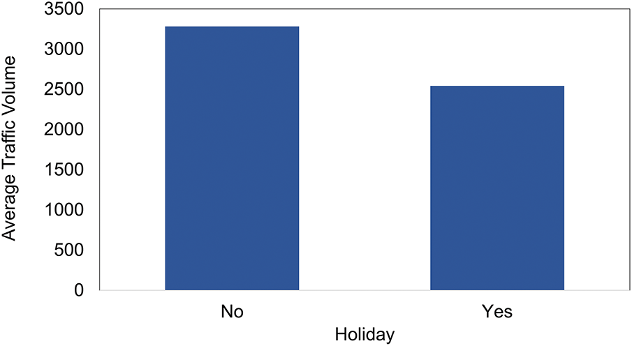
Figure 5: Comparison of average traffic volume on holidays and non-holidays
The Pearson correlation heatmap in Fig. 6 illustrates the linear relationships between traffic volume and the numerical features of the original MITV dataset, including temperature, rain_1h, snow_1h, and clouds_all. From the perspective of mathematics, Pearson’s correlation coefficient, ranging from −1 to 1, measures the strength and direction of linear associations: values close to −1 reflect a strong negative correlation, values near 1 indicate a strong positive correlation, and values around 0 imply little to no linear association.
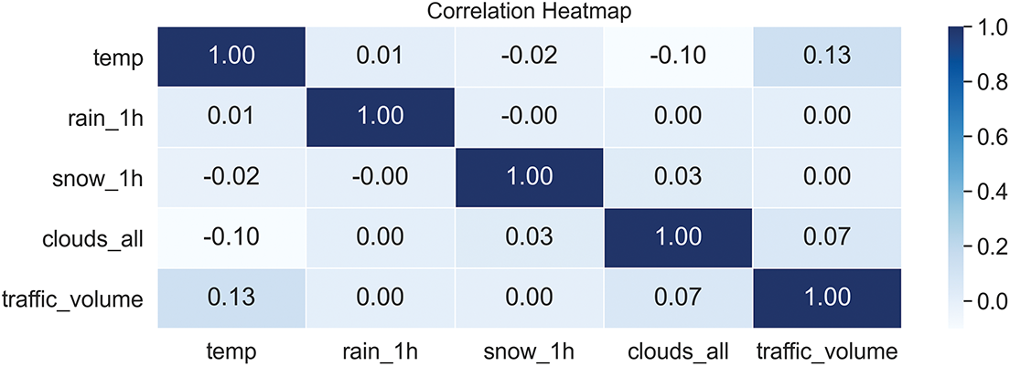
Figure 6: Heatmap of traffic volume and numerical features
Among the analyzed features, temperature shows the highest positive correlation with traffic volume (0.13), while clouds_all follows with a weaker positive correlation (0.07). Meanwhile, rain_1h and snow_1h exhibit near-zero correlations, indicating minimal direct influence on traffic volume. Furthermore, the low correlations observed between the numerical features themselves suggest the absence of multicollinearity, supporting their suitability as independent predictors for the modeling process.
To identify the most influential attributes for predicting traffic volume after preprocessing the MITV dataset, a feature importance method based on mutual information (MI) was applied to assess linear and nonlinear relationships between each feature and the target variable traffic volume. The resulting ranked list, presented in Fig. 7, reveals that hour (1.413), temperature (0.401), and weekday (0.257) are the top three contributors. These attributes reflect key temporal and environmental patterns that competently influence traffic flow. In contrast, features such as holiday (0.008) and snow_1h (0.004) exhibit negligible correlation scores, consistent with their minimal relevance observed in the correlation heatmap. These results identify variables with the highest predictive potential for traffic volume modeling.
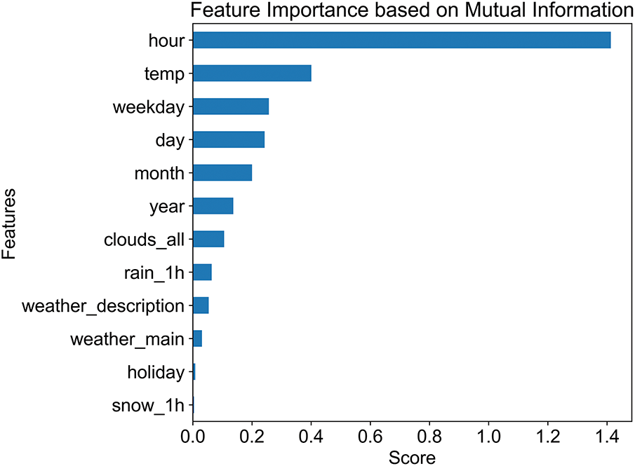
Figure 7: Features ranked by mutual information with traffic volume in the MITV dataset
The REPTF-TMDI method was implemented in C#, utilizing the WEKA machine learning library [51] for model construction and evaluation. All experiments were carried out on a standard desktop computer equipped with an Intel® CoreTM i7 processor (1.90 GHz) and 8 GB of RAM. For traffic flow prediction, this study employed a Bagging ensemble approach with REPTree as the base classifier. The specific configurations used in the experiments are detailed below:
• Bagging configuration: For ensemble learning, Bagging technique was employed with REPTree as the base learner. The “bagSizePercent” was set to 100, meaning that each model in the ensemble was trained on a bootstrapped sample equivalent in size to the original training dataset. The “batchSize” was set to 100, indicating the number of instances processed per batch during training. The “calcOutOfBag” flag was set to false, so out-of-bag error estimates were not calculated. The ensemble used 10 execution “numExecutionSlots” for parallel model building, and the “seed” was set to 1 to ensure reproducibility in the random processes. Furthermore, advanced features like “storeOutOfBagPredictions” and “representCopiesUsingWeights” were turned off, meaning that each bootstrap sample was handled independently without storing extra prediction metadata or using weighted instance representations.
• REPTree configuration: The “batchSize” was set to 100, defining the number of instances processed per batch during training. The tree’s growth was unrestricted in terms of depth, with “maxDepth” set to −1, allowing it to expand fully based on the data and stopping conditions. To avoid overly specific leaf nodes, the “minNum” parameter was set to 2, enforcing a minimum of two instances per leaf. The “minVarianceProp”, which defines the minimum variance proportion required for a split to be considered meaningful, was set to 0.001. Tree pruning was enabled by setting “noPruning” with a false value to reduce the risk of overfitting. The “initialCount” parameter was set to 0.0, meaning no artificial inflation of instance counts was applied at the beginning of training. Capability checks were not skipped, as indicated by “doNotCheckCapabilities” with a false value. The model used 3-fold cross-validation with “numFolds” set to 3 for internal reduced-error pruning. Additionally, the “spreadInitialCount” option was set to false, indicating that the initial count was not distributed across the leaves during training to preserve the original instance distribution.
To quantitatively assess the success of the proposed REPTree Forest with time-based missing data imputation (REPTF-TMDI), we employed a set of standard regression evaluation metrics. The proposed method’s performance was validated across multiple evaluation metrics, including mean absolute error (MAE), correlation coefficient (R), relative absolute error (RAE), root mean squared error (RMSE), and root relative squared error (RRSE), ensuring the reliability of the findings. These metrics provide comprehensive insights into the predictive accuracy, error magnitude, and relative performance of the model. Each metric captures a different aspect of the model’s efficacy, enabling a robust evaluation across various experimental conditions. The mathematical definitions of these metrics are provided in Eqs. (6)–(10). Let
• Correlation coefficient (R): The correlation coefficient measures how strongly the predicted values align with the actual values in terms of a linear relationship, indicating both the degree and direction of this association.
• Mean absolute error (MAE): This metric quantifies the average magnitude of prediction errors by calculating the mean of the absolute differences between actual and predicted values, regardless of the direction of the errors.
• Root mean squared error (RMSE): It is defined as the square root of the average squared differences between the predicted and actual values, placing greater emphasis on larger errors compared to the MAE.
• Relative absolute error (RAE): This metric evaluates the total absolute prediction error in relation to the total absolute deviation of the actual values from their mean, providing a normalized measure of model accuracy.
• Root Relative Squared Error (RRSE): It measures the prediction error relative to a simple baseline model by comparing the root of the squared prediction errors to the root of the squared deviations from the actual mean.
5.1 Missing Data Visualization
This subsection provides a visual analysis of the missing data patterns and demonstrates the effectiveness of the proposed TMDI imputation approach under varying levels of missingness. Fig. 8 displays the missing data patterns under various levels of artificially introduced missingness using the “ReplaceWithMissingValue” filter in WEKA. Each subplot, Fig. 8a–h, shows a heatmap of the dataset with increasing percentages of missing data. The blue color indicates complete data, while the white color shows the missing values. The sparkline on the right side of each figure offers an overview of data completeness, representing the rows with the highest and lowest levels of missing data. For instance, in Fig. 8h, the greatest degree of missingness occurs when only a single feature—the target variable—is retained. In all figures, the maximum completeness value is 13, indicating that all features were fully observed in those rows. The missing data is spread across all features relatively uniformly, implying a random missingness pattern. As the percentage of missing data increases from 5% to 40%, the heatmaps show a progressively higher number of gaps. After applying the TMDI method, the imputation of the missing values was performed completely.
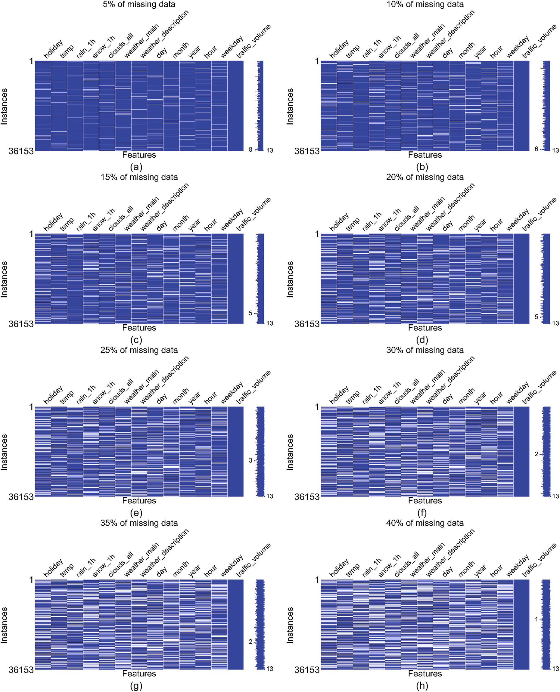
Figure 8: Data patterns observed under varying missing data ratios
5.2 Impact of Missing Data Rates on REPTF-TMDI
This subsection presents a comprehensive analysis of the REPTF-TMDI method under varying levels of data incompleteness. To assess its quality, we conducted extensive experiments on the MITV dataset. We employed a 75%–25% split tailored to the temporal nature and sequential structure of the data, ensuring that earlier time points were used exclusively for training while the most recent data was reserved for testing, thereby maintaining temporal causality and enabling realistic out-of-sample forecasting. Following preprocessing, our final dataset included 13 features, among which traffic-volume served as the target variable for the regression task. The remaining 12 input features comprised temporal attributes (day, month, year, hour, weekday, holiday), meteorological data (temperature, snow_1h, rain_1h, clouds_all), and weather descriptors (weather-main and weather-description). The final dataset consisted of 48,204 instances, forming a data matrix with 626,652 individual cells (48,204 rows × 13 features).
In order to simulate various real-world data loss scenarios, we introduced missing values at controlled rates using WEKA’s “ReplaceWithMissingValue” filter. This filter replaces attribute values with missing entries based on a specified probability, efficiently simulating missing data by flipping a biased coin for each cell. Importantly, the class attribute (traffic-volume) is left intact. We applied the filter at eight different missing data rates, namely 5%, 10%, 15%, 20%, 25%, 30%, 35%, and 40%, resulting in a progressive removal of values from approximately 21,664 to over 173,623 input cells. For example, when the “probability” hyperparameter is set to 0.4, it indicates that 40% of the values will be replaced with missing ones. Although the “attributeIndices” hyperparameter was set to “first-last”, the class attribute (traffic-volume) remained unchanged, as the procedure inherently ignores target values. To ensure consistent and reproducible results across runs, a constant random seed was used throughout all experiments. Specifically, the seed was set to 1. The core of our methodology involved imputing these missing values using our proposed TMDI technique, followed by applying the REPTree Forest ensemble for regression. We evaluated prediction capability using five standard metrics, including R, MAE, RMSE, RAE, and RRSE. The results, summarized in Table 6, reliably determine the dominance of REPTF-TMDI across all missing data rates.
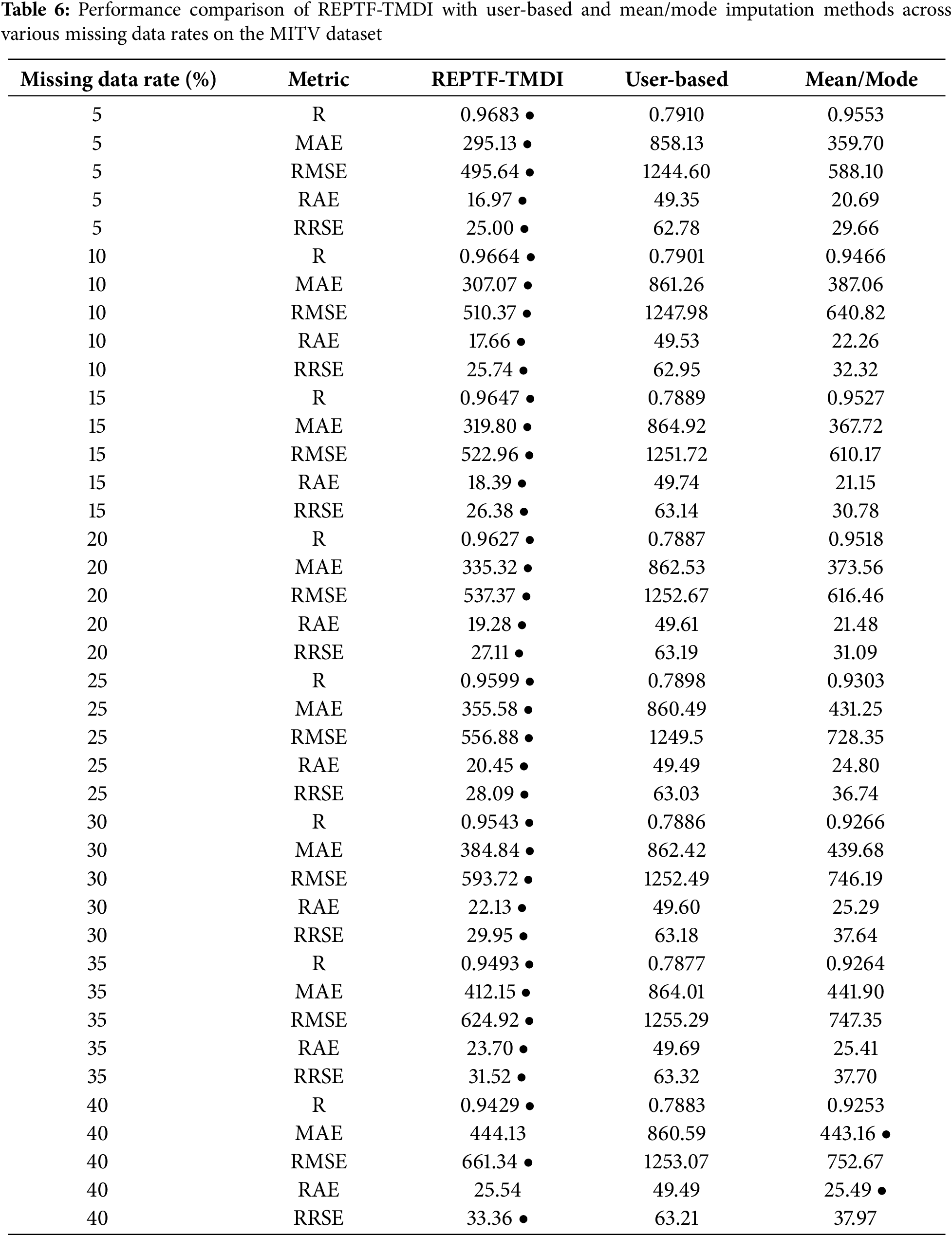
To benchmark TMDI’s efficacy, we compared it with two widely used imputation strategies in WEKA, including the user-based method, which replaces all missing values with a user-specified constant via the “ReplaceMissingWithUserConstant” filter, and the mean/mode method, which fills missing numeric and nominal values using means and modes of training data through the “ReplaceMissingValues” filter. For each missing rate, we applied these baseline imputation methods, followed by REPTree Forest for regression. As clearly illustrated in Table 6, the REPTF-TMDI method outperformed both existing approaches, with the (●) symbol marking its superior productivity. For example, at the lowest missing rate (5%), REPTF-TMDI achieved R = 0.9683, MAE = 295.13, RMSE = 495.64, RAE = 16.97, and RRSE = 25.00, far exceeding the user-based method (R = 0.7910) and mean/mode (R = 0.9553). Even at a high missing rate of 35%, REPTF-TMDI maintained R = 0.9493 and MAE = 412.15, compared to R = 0.7877 and MAE = 864.01 for the user-based method. Notably, REPTF-TMDI preserved strong predictive capabilities up to 40% missingness, showing only a moderate rise in various metrics. In short, the REPTF-TMDI method outperformed conventional imputation techniques by achieving an average 11.76% improvement in terms of R.
We also tested the REPTree Forest model alone (without any missing value imputation) on the original, complete MITV dataset. This serves as the output upper bound, achieving R = 0.9695, MAE = 289.26, RMSE = 486.27, RAE = 16.64, and RRSE = 24.53. Compared to this benchmark, our REPTF-TMDI model, even under substantial missing-ness (e.g., 25%–30%), shows only minor degradation, underlining the robustness of TMDI in reconstructing lost information and preserving regression accuracy.
The empirical results validate the resilience of REPTF-TMDI under varying degrees of missing data. The model not only maintained high precision close to the upper bound of the complete-data scenario but also considerably outperformed traditional imputation strategies. These findings confirm its suitability for real-world traffic prediction applications where data incompleteness is a predominant issue.
Two statistical tests were employed to assess the significance of the correlation coefficient (R) results given in Table 6. The Friedman Aligned Ranks Test [52] yielded a p-value of 0.00078, while the Quade Test [53] produced an even smaller p-value of 0.00002. Since both p-values are well below the α = 0.05 significance threshold, the null hypotheses (H0), which assume no difference between the groups, are rejected for both tests. These findings indicate statistically significant differences among the compared models. According to confidence intervals, a p-value less than 0.01 is considered “highly significant”, indicating very strong evidence against the null hypothesis and confirming that the difference between REPTF-TMDI and other models is statistically meaningful.
5.3 Actual vs. Predicted Values
To further demonstrate the accuracy of the proposed REPTF-TMDI method, we present visual comparisons between actual and predicted traffic volume values under various temporal conditions. These sample visualizations serve as qualitative support for the quantitative metrics reported in the previous subsection. Fig. 9 displays actual and predicted daily traffic volumes for the entire month of September 2018. The close alignment of the two plots indicates that REPTF-TMDI captures the temporal dynamics and daily traffic fluctuations effectively. Despite the natural variability in traffic patterns across days, the model consistently follows the actual values, confirming its stability over a long time span.
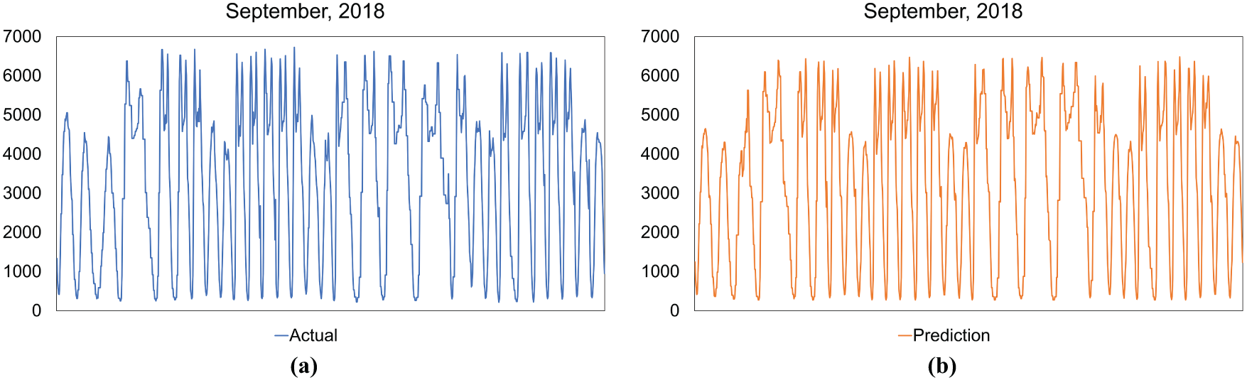
Figure 9: Comparison of actual (a) and predicted (b) hourly traffic volumes for September 2018 using REPTF-TMDI
To explore results under different traffic conditions, Fig. 10 shows two representative daily profiles, one from a weekday (Fig. 10a) and one from a weekend (Fig. 10b). These examples demonstrate the method’s ability to adapt to different traffic patterns—characterized by sharper morning and evening peaks on weekdays, and a more gradual curve on weekends. These plots demonstrate the flexibility of REPTF-TMDI in correctly capturing the distinct traffic conditions observed across different day types. In both cases, the actual traffic volumes are closely tracked, with minimal deviation during high-variance hours.
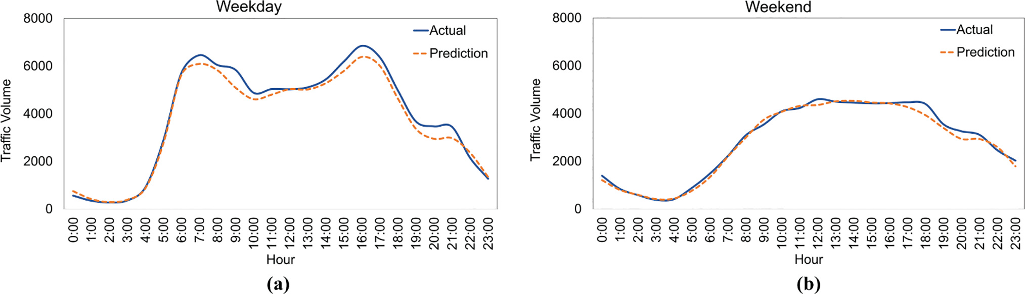
Figure 10: Sample comparisons of actual and predicted traffic volumes on (a) a typical weekday and (b) a weekend day using REPTF-TMDI
Finally, Fig. 11 displays a scatter plot comparing actual and predicted values for the 2017–2018 period of the dataset. The dense diagonal alignment of points depicts a strong linear correlation between actual and predicted traffic volumes. The spread around the diagonal remains narrow even for higher traffic volumes, further validating the method’s performance across the full range of data. These visual analyses provide compelling evidence of REPTF-TMDI’s capability, even under varying temporal conditions and traffic behaviors.
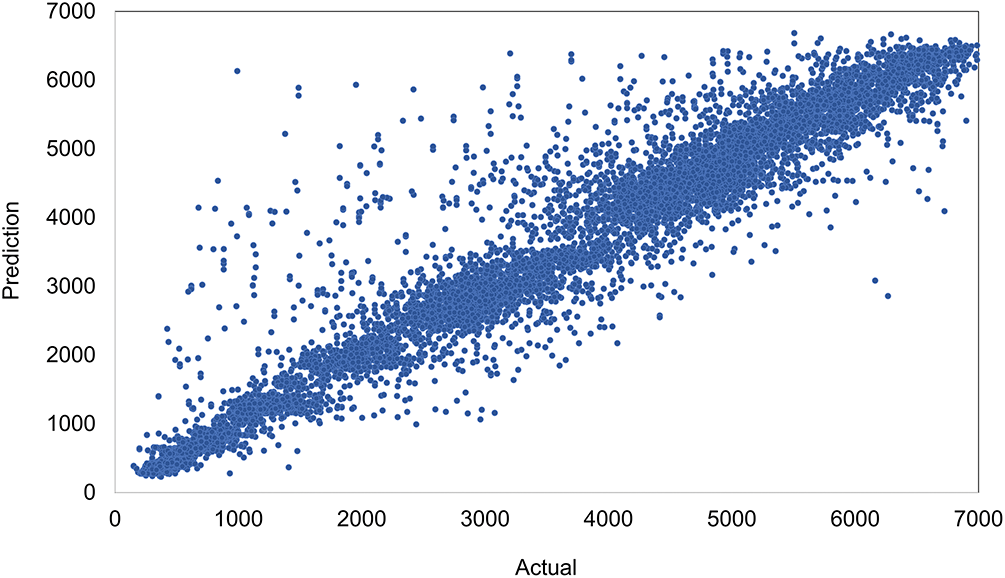
Figure 11: Scatter plot of actual and predicted traffic volumes across the 2017–2018 period using REPTF-TMDI
To illustrate how the REPTree Forest operates within the proposed REPTF-TMDI method, Fig. 12 provides a representative decision tree. This tree exemplifies how the model utilizes both temporal and weather-related features to predict traffic volume. Internal nodes denote decision points based on attributes such as hour, weekday, day, month, holiday, temperature, cloud coverage, weather main, and weather description, while the leaf nodes contain the predicted traffic volume for each path of conditions. This analysis was conducted over the MITV dataset, which spans hourly traffic and weather data from 2012 to 2018, to predict traffic volume under varying contextual conditions. The structure proficiently captures recurring temporal patterns that influence traffic behavior. For instance, one branch indicates that at 5:00 AM on Sundays, the predicted traffic volume is approximately 524.31 vehicles, whereas another path shows that on Tuesday afternoons at 4:00 PM when it is not a holiday, traffic volume peaks at around 6412.1 vehicles—suggesting a weekday rush hour effect. Other segments of the tree reveal more granular patterns, such as the combination of 2:00 AM on Mondays during the 30th of the month, with “clouds_all” as the primary weather condition, resulting in a predicted volume of 260 vehicles. Beyond temporal variables, the tree also incorporates detailed weather conditions, showing their impact on traffic flow. For example, on Wednesdays at 4:00 PM, if the weather is described as a “proximity thunderstorm”, the model forecasts a volume of 5530 vehicles, which increases to 5846.5 in the presence of “mist”. The tree also handles numerical thresholds for continuous features, such as predicting different volumes based on temperature (e.g., temp < 278.46) and cloud density (clouds_all ≥ 45.5), allowing the model to account for more subtle environmental effects. This illustrative tree emphasizes the interpretability and predictive power of the REPTF-TMDI method. It clearly demonstrates how the model integrates multiple dimensions of temporal and environmental information to capture intricate traffic flow dynamics. As part of the broader framework, this decision structure showcases the value of ensemble learning combined with time-based missing data imputation in producing meticulous, explainable, and robust traffic predictions.
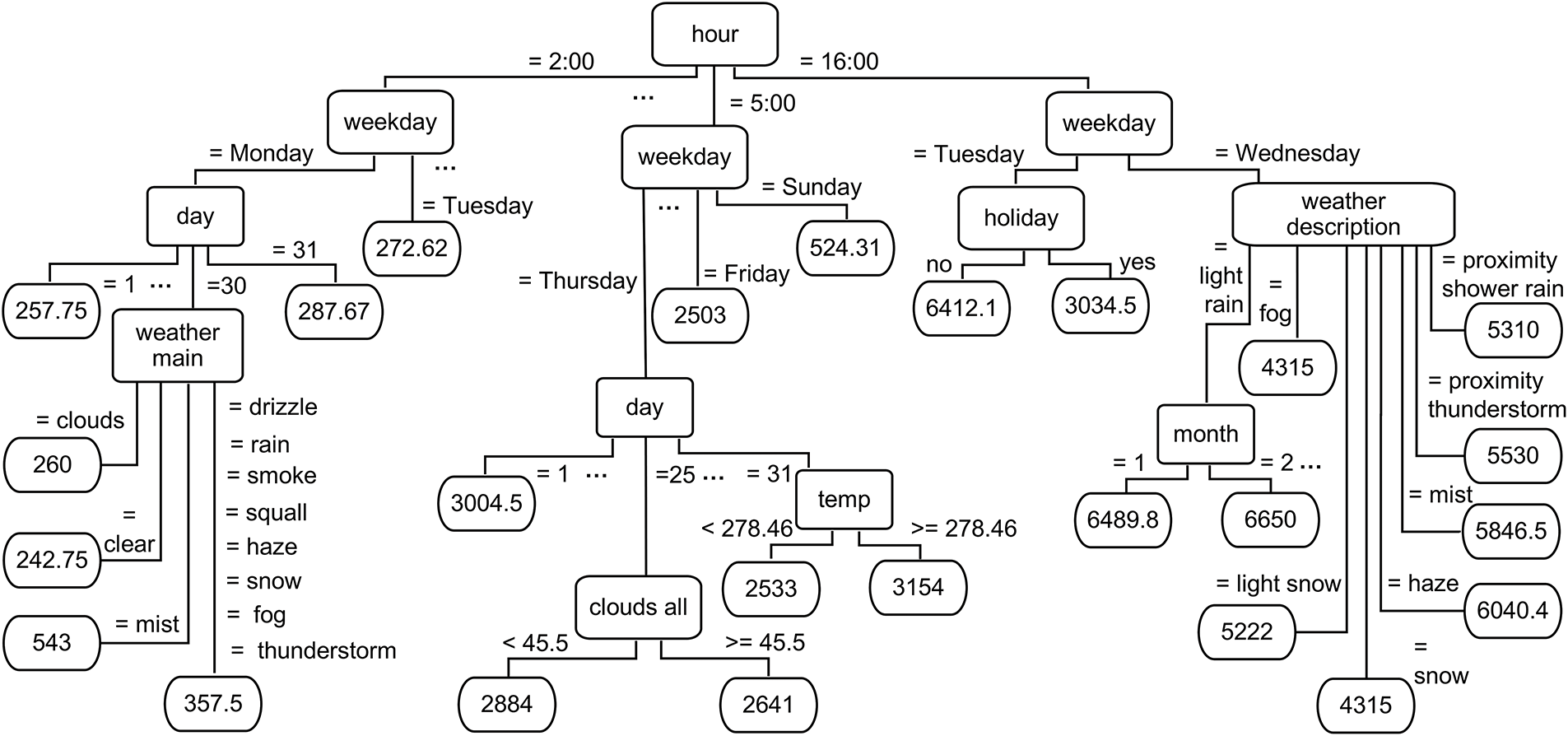
Figure 12: Sample REPTree showing how features guide traffic volume prediction in the MITV dataset
6.1 Comparison with Recent Studies
To evaluate the success of the proposed REPTree Forest, a comprehensive comparison was conducted against several state-of-the-art studies to predict traffic volume over the same MITV dataset. These studies represent a variety of regression paradigms, including tree-based models, imputation-driven techniques, deep neural networks, and ensemble approaches [54–58]. Further studies integrating deep learning, data reduction, or model optimization strategies were also taken into account [59–63]. Finally, studies exploring various regression strategies and domain-specific forecasting applications were included [64–67]. The results, summarized in Table 7, demonstrate that REPTree Forest consistently outperformed all compared methods across the three primary evaluation metrics, including MAE, R, and RMSE. In terms of error metrics, REPTree Forest attained the lowest values—MAE of 289.26 and RMSE of 486.27—among all evaluated methods. Compared to state-of-the-art methods, the proposed model achieved an average improvement of 68.62% in RMSE and 70.52% in MAE. Specifically, our model achieved an R score of 0.9695, significantly surpassing competitive baselines such as TPOT Regressor [67] (R2 = 0.9250) and LuPTS ReLU RF [64] (R2 = 0.9100), reflecting exceptional predictive accuracy. These significant margins prove the success of our model in reducing prediction errors while substantially increasing the goodness-of-fit and ensuring more reliable predictions for sustainable urban mobility.
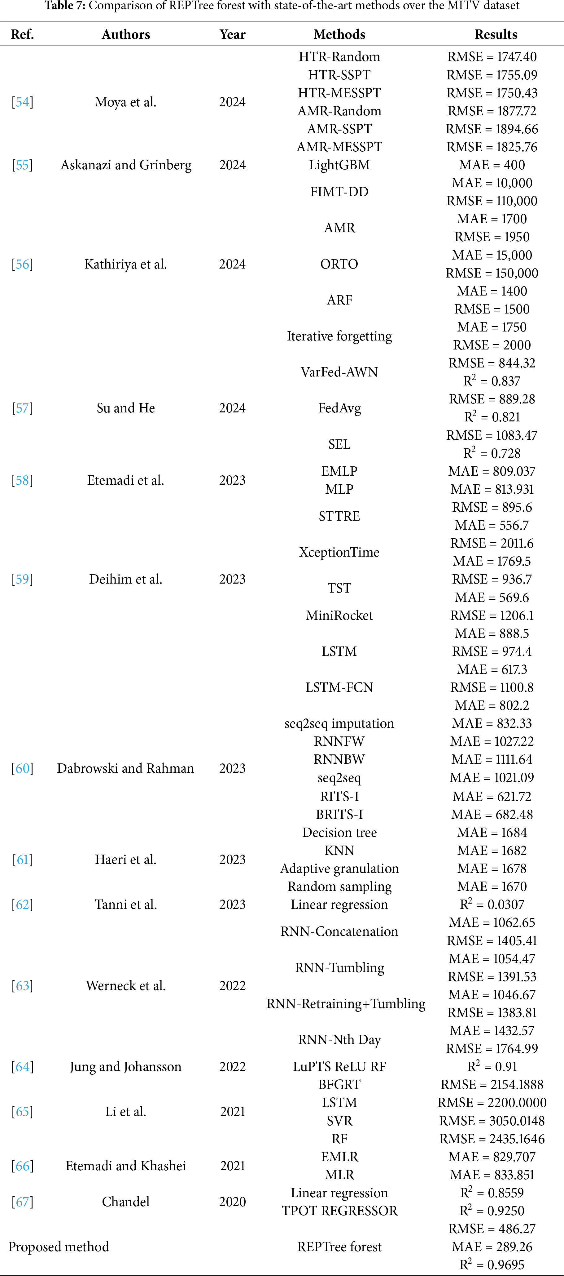
Notably, compared to recent federated and deep learning approaches like VarFed-AWN [57] (RMSE = 844.32) and STTRE [59] (RMSE = 895.6), our method reveals a 42%–45% reduction in RMSE. Even advanced adaptive models such as ARF and FIMT-DD [56], which are designed for online learning and drift adaptation, reported meaningfully higher error rates (e.g., ARF: MAE = 1400, RMSE = 1500), suggesting that conventional model drift mechanisms may be less competent when confronted with substantial missing data. Furthermore, deep learning models such as LSTM, LSTM-FCN, and time series transformers [59] exhibited larger MAE and RMSE values, underlining the inherent difficulty of tuning such models in noisy or incomplete time-series environments. Our approach also outperformed imputation-based architectures like RITS-I (MAE = 621.72) and BRITS-I (MAE = 682.48) [60]. Overall, the substantial enhancements across all key metrics validate the methodological innovations in the proposed model and affirm its suitability for real-world traffic flow prediction tasks, especially in the context of sustainable transportation systems, where missing data is a prevalent challenge.
6.2 Comparison with Alternative Methods
In addition to the comparisons mentioned above, to show the effectiveness of the proposed method, we conducted a comparative evaluation with four widely used algorithms: random forest, k-nearest neighbors (KNN), decision stump, and random tree. All models were executed under the same experimental conditions using the MITV dataset to guarantee a consistent evaluation. As shown in Table 8, the proposed method outperformed the other models in all performance metrics. Particularly, it attained the highest R score (R = 0.9695), indicating a strong agreement between the predicted and actual traffic flow values. Furthermore, it recorded the lowest error values, including MAE at 289.26, RMSE at 486.27, RAE at 16.64, and RRSE at 24.53. These results confirm the model’s robustness and precision.
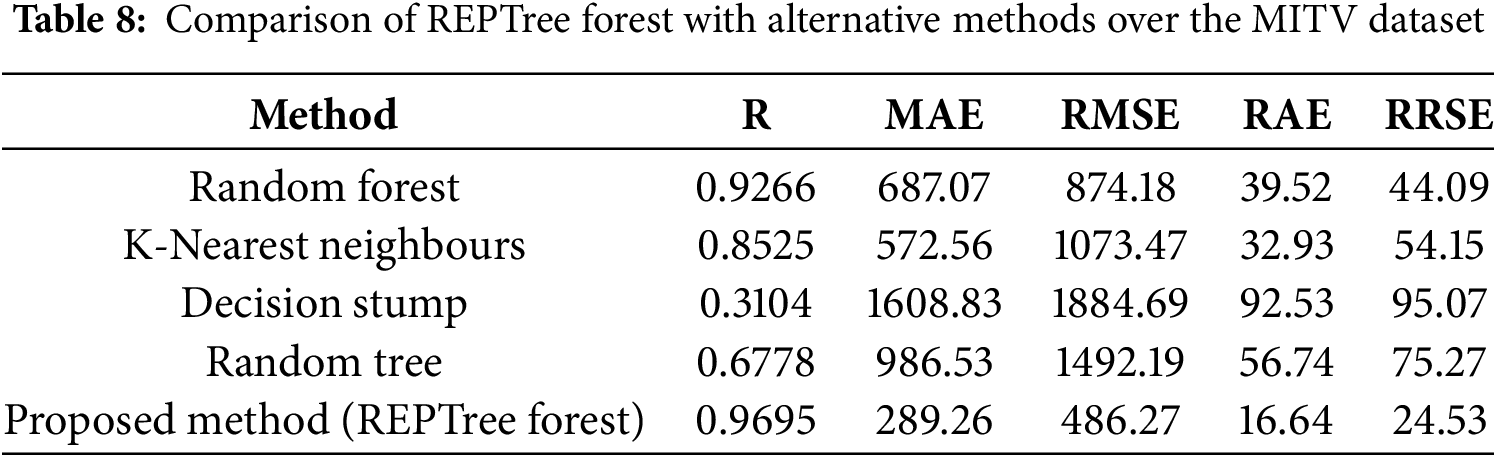
Among the alternatives, random forest displayed a relatively high R score with 0.9266; however, it revealed substantially higher error rates with MAE = 687.07 and RMSE = 874.18, when compared to our proposed method. The KNN algorithm showed moderate performance (R = 0.8525), but with elevated RMSE (1073.47), indicating reduced reliability under data sparsity. The decision stump algorithm performed the weakest, with a very low R score (R = 0.3104) and the highest RMSE (1884.69), revealing its inadequacy for modeling complex patterns in the data. Random tree performed better than decision stump (R = 0.6778) but still lacked the predictive accuracy and consistency demonstrated by the proposed model. These results showcase that the proposed method offers superior prediction accuracy and generalization ability in the presence of missing data, making it greatly suitable for traffic flow prediction tasks.
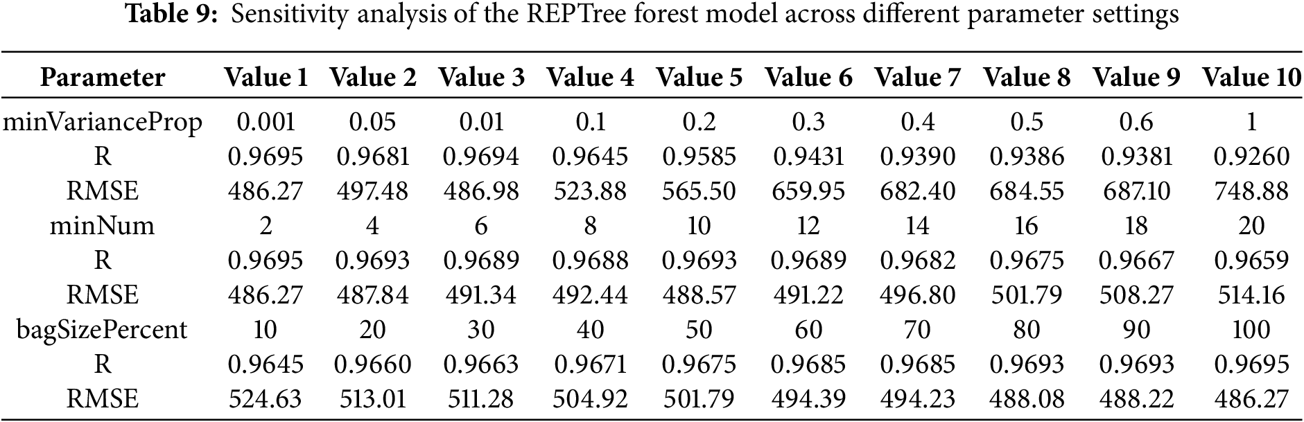
To further evaluate the model’s performance, a sensitivity analysis was performed using different values for the parameters of the REPTree Forest, as shown in Table 9. The minimum variance proportion (minVarianceProp) required for a node to split, was tested across values from 0.001 to 1. As this parameter increased, R declined while RMSE rose sharply, indicating that excessive variance requirements led to underfitting and overly shallow trees. The minimum number of instances per leaf (minNum) was varied from 2 to 20. Smaller values allowed for more flexible and detailed splits, whereas larger values limited the tree’s ability to capture patterns, generally reducing accuracy. Lastly, the bag size percentage (bagSizePercent), which determines the proportion of training data used per iteration, was evaluated from 10% to 100%. Higher values consistently improved model robustness, while smaller subsets introduced greater variance in predictions. These results confirm that the REPTree Forest achieved its best performance when allowed to grow deeper trees and when trained on larger samples.
6.4 Survey of the Generalizability
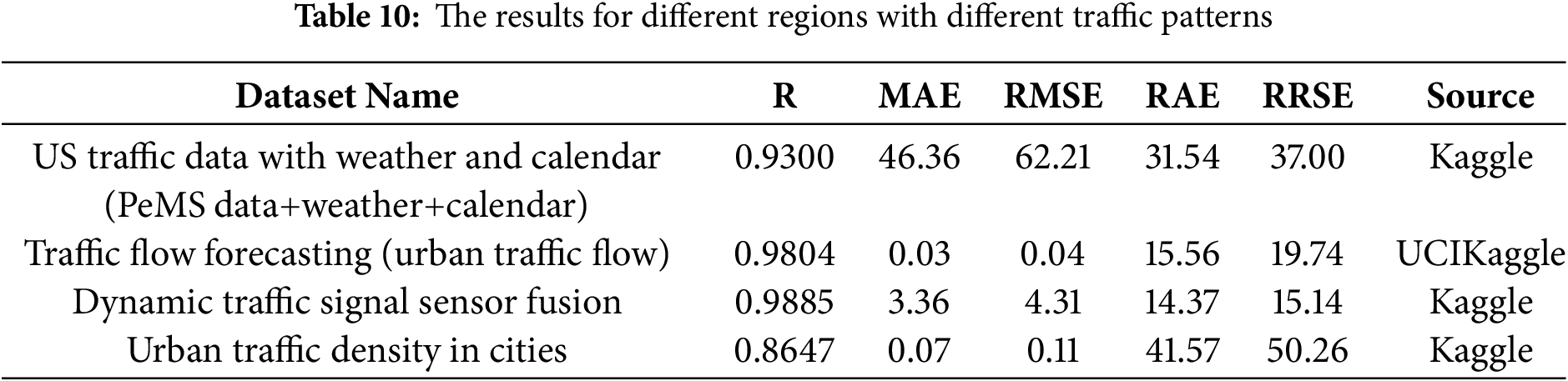
To address concerns regarding the generalizability of the approach beyond the MITV dataset, the evaluation was extended to include four supplementary traffic datasets from different geographic regions. These datasets represent urban environments such as Los Angeles and the Northern Virginia/Washington D.C. capital region, capturing diverse traffic dynamics and regional weather conditions. The proposed model consistently demonstrated strong predictive performance across these datasets, with R values ranging from 0.86 to 0.98 and RMSE values as low as 0.04. A detailed summary of key metrics, namely MAE, RAE, and RRSE, is presented in Table 10 to provide further validation of the model’s outperformance. The diversity of dataset sources, from Kaggle to UCI public repositories, has reinforced the claim of cross-regional applicability. Although these datasets exhibit various scales and temporal structures, high accuracy was still maintained. Through this cross-dataset validation, the REPTF-TMDI model’s adaptability to varying urban traffic contexts has been confirmed. Overall, the results substantiate the generalizability of REPTF-TMDI beyond the original MITV setting.
To further support the applicability of the model, datasets containing a richer set of contextual features beyond the original MITV attributes were also explored. These additional variables included environmental factors (e.g., dew point, humidity, pressure, wind speed, and direction), road characteristics (e.g., location, direction, number of lanes), and vehicle-specific information (e.g., type of vehicle such as ambulance, bus, truck, or emergency services). In some datasets, radar-based traffic indicators—such as average vehicle speed and traffic signal duration classes—were also available. The model delivered strong performance across these feature-enriched datasets, indicating promising potential for real-world scenarios.
To address concerns regarding the use of artificially generated missing data, the REPTF-TMDI method was also applied to the US traffic data with weather and calendar information, which contains naturally occurring real-world missing values. The proposed method maintained high performance on this dataset, achieving an R value of 0.93 along with low error metrics (MAE = 46.36, RMSE = 62.21), thereby confirming its effectiveness under authentic missingness conditions. These results indicate that the model can manage not only synthetically masked inputs but also naturally incomplete data, further reinforcing the practical credibility of REPTF-TMDI in traffic forecasting.
7 Conclusions and Future Works
This study introduces the novel REPTF-TMDI method, which combines the strengths of reduced error pruning tree forest (REPTree Forest) and time-based missing data imputation (TMDI) to address the challenges of traffic flow prediction with missing data. The major contributions of this work include the presentation of the REPTree Forest as an ensemble learning model for improving predictive accuracy, the proposal of the TMDI method tailored for time-related traffic datasets, and the introduction of the hybrid REPTF-TMDI method, which is the first of its kind in the literature. The method is evaluated using the metro interstate traffic volume (MITV) dataset, covering 48,204 hourly records from 2012 to 2018, and various missing data rates (5% to 40%) are simulated. In addition to the MITV dataset, four supplementary datasets from diverse regions and contexts were also employed to assess the model’s performance under various traffic patterns. The consistently strong results obtained across all datasets confirm the robustness and generalizability of the proposed approach.
When compared to conventional imputation techniques, such as mean/mode and user-based imputation, the REPTF-TMDI method demonstrated notable outperformance, with an average 11.76% improvement in R. Furthermore, when compared with 14 state-of-the-art studies, REPTree Forest showed a 68.62% improvement in RMSE and a 70.52% improvement in MAE. Additionally, the integration of temporal and environmental feature importance analysis using mutual information provided valuable perceptions of the key factors influencing traffic flow prediction. Features such as hour of the day (1.413), temperature (0.401), and weekday (0.257) were identified as the most influential, while features like holiday (0.008) and snow_1h (0.004) exhibited minimal impact.
Despite the comprehensive analysis and promising results, the study presents several limitations that warrant further reflection. One concern lies in the reliance on differences between artificially generated and real data gaps, which may not fully capture the real-world missing data scenarios. Among the five datasets used in the evaluation, only one contains naturally occurring missing data, while the remaining four are based on synthetically introduced gaps. Expanding the analysis to include a broader range of real-world missing data cases would further enhance the value of the work. Additionally, although the proposed method demonstrated strong performance across several regions, assessing its generalizability to a wider range of geographical contexts and varying traffic conditions would further strengthen its contribution to the field.
Building on the strong performance of the REPTF-TMDI method, future research could focus on integrating it into real-time scenarios, enabling dynamic forecasting and decision-making. This could significantly improve urban mobility by providing more responsive traffic flow predictions in real-time environments. Additionally, future research could explore incorporating additional feature data, such as vehicle type data, to investigate their impact on traffic flow prediction. Furthermore, implementing the REPTF-TMDI method in mobile applications or cloud-based platforms could prove valuable, principally within the context of smart cities and large-scale transportation infrastructure. Such developments could supplementary reveal its versatility in tackling various missing data challenges across traffic concerns, contributing to broader sustainability goals by advancing eco-friendly urban transportation and promoting responsible urban development.
Acknowledgement: Not applicable.
Funding Statement: The authors received no specific funding for this study.
Author Contributions: The authors confirm contribution to the paper as follows: Conceptualization, Bita Ghasemkhani, Yunus Dogan and Goksu Tuysuzoglu; methodology, Bita Ghasemkhani, Yunus Dogan and Goksu Tuysuzoglu; software, Goksu Tuysuzoglu; validation, Goksu Tuysuzoglu and Elife Ozturk Kiyak; formal analysis, Bita Ghasemkhani; investigation, Bita Ghasemkhani, Yunus Dogan and Kokten Ulas Birant; resources, Goksu Tuysuzoglu, Elife Ozturk Kiyak, Semih Utku and Kokten Ulas Birant; data curation, Semih Utku; writing—original draft preparation, Bita Ghasemkhani; writing—review and editing, Goksu Tuysuzoglu, Yunus Dogan, Elife Ozturk Kiyak, Semih Utku, Kokten Ulas Birant and Derya Birant; visualization, Yunus Dogan, Goksu Tuysuzoglu and Elife Ozturk Kiyak; supervision, Derya Birant; project administration, Derya Birant; funding acquisition, Goksu Tuysuzoglu, Yunus Dogan, Elife Ozturk Kiyak, Semih Utku, Kokten Ulas Birant and Derya Birant. All authors reviewed the results and approved the final version of the manuscript.
Availability of Data and Materials: The metro interstate traffic volume (MITV) dataset that supports the findings of this study is openly available in the UCI Machine Learning Repository [50] at https://doi.org/10.24432/C5X60B and https://archive.ics.uci.edu/dataset/492/metro+interstate+traffic+volume (accessed on 22 April 2025). Furthermore, four supplementary datasets used for evaluating the generalizability of the proposed method are publicly accessible as follows:
• The US traffic data with weather and calendar (PeMS data+weather+calendar) dataset is available on Kaggle [68] at https://www.kaggle.com/datasets/maryamshoaei/us-traffic-data-with-weather-and-calendar-dataset (accessed on 24 July 2025).
• The traffic flow forecasting (Urban Traffic Flow) dataset is available from both UCI and Kaggle [69] at https://ar-chive.ics.uci.edu/dataset/608/traffic+flow+forecasting or https://www.kaggle.com/datasets/jvthunder/urban-traffic-flow-csv (accessed on 24 July 2025).
• The dynamic traffic signal sensor fusion dataset is hosted on Kaggle [70] at https://www.kaggle.com/datasets/zoya77/dynamic-traffic-signal-sensor-fusion-dataset (accessed on 24 July 2025).
• The urban traffic density in cities dataset is available on Kaggle [71] at https://www.kaggle.com/datasets/tanishqdublish/urban-traffic-density-in-cities (accessed on 24 July 2025).
Ethics Approval: Not applicable.
Conflicts of Interest: The authors declare no conflicts of interest to report regarding the present study.
Abbreviations
| AE | Absolute error |
| AMR | Adaptive model rules |
| ANN | Artificial neural network |
| ARF | Adaptive random forests |
| ARIMA | Autoregressive integrated moving average |
| ATR | Automatic traffic recorder |
| AWN | Aggregation weight neural networks |
| Bagging | Bootstrap aggregating |
| BFGRT | Boosted fuzzy granular regression trees |
| BGRU | Bidirectional gated recurrent unit |
| BILSTM | Bidirectional long short-term memory |
| BRITS-I | Bidirectional recurrent imputation for time series-improved version |
| CL | Centralized learning |
| CNN | Convolutional neural networks |
| DT | Decision tree |
| EC | Equilibrium coefficient |
| ELM | Extreme learning machine |
| EMLP | Etemadi multi-layer perceptron |
| EMLR | Etemadi multiple linear regression |
| EN | ElasticNet |
| ENN | Elman neural network |
| EV | Explained variance |
| EWM | Entropy weight method |
| FCM | Fuzzy c-means clustering algorithm |
| FedAvg | Federated averaging |
| FIMT-DD | Fast incremental model trees with drift detection |
| FL | Federated learning |
| GA | Genetic algorithm |
| GB | Gradient boosting |
| GBR | Gradient boosting regressor |
| GRU | Gated recurrent units |
| HTR | Hoeffding tree regressor |
| KNN | K-nearest neighbors |
| LightGBM | Light gradient boosting machine |
| LR | Logistic regression |
| LS-SVM | Least-squares support vector machines |
| LSTM | Long short-term memory |
| LSTM-FCN | Long short-term memory-fully convolutional network |
| LuPTS ReLU RF | Learning using privileged time series-rectified linear activation unit-random Fourier |
| MAE | Mean absolute error |
| MAPE | Mean absolute percentage error |
| MDI | Missing data imputation |
| MESSPT | Micro-evolutionary single-pass self-hyper-parameter tuning |
| MiniRocket | Minimally random convolutional kernel transform |
| MITV | Metro interstate traffic volume |
| ML | Machine learning |
| MLP | Multi-layer perceptron |
| MLPR | Multi-layer perceptron regression |
| MLR | Multiple linear regression |
| MSE | Mean squared error |
| NAR | Nonlinear autoregressive neural networks |
| NB | Naive Bayes |
| NN | Neural networks |
| ORTO | Online regression trees with options |
| POA | The pelican optimization algorithm |
| RAE | Relative absolute error |
| REPTF-TMDI | Reduced error pruning tree forest with time-based missing data imputation |
| REPtree | Reduced error pruning tree |
| REPTree Forest | Reduced error pruning tree forest |
| ResNet | Residual convolutional neural network |
| RF | Random forest |
| RFR | Random forest regression |
| RITS-I | Recurrent imputation for time series-improved version |
| RMSE | Root mean square error |
| RNN | Recurrent neural network |
| RNNBW | Recurrent neural network backward decoder |
| RNNFW | Recurrent neural network forward decoder |
| RRSE | Root relative squared error |
| SEL | Stacking-based ensemble learning |
| seq2seq | Sequence-to-sequence |
| SGR | Stochastic gradient regressor |
| SMAPE | Symmetric mean absolute percentage error |
| SSPT | Single-pass self-hyper-parameter tuning |
| STTRE | Spatio-temporal transformer with relative embedding |
| SVM | Support vector machine |
| SVR | Support vector regression |
| TFP | Traffic flow prediction |
| TMDI | Time-based missing data imputation |
| TPOT | Tree-based pipeline optimization tool |
| TST | Time series transformer |
| VAR | Vector autoregressive model |
| XGBoost | Extreme gradient boosting |
References
1. Medina-Salgado B, Sánchez-DelaCruz E, Pozos-Parra P, Sierra JE. Urban traffic flow prediction techniques: a review. Sustain Comput Inform Syst. 2022;35(7):100739. doi:10.1016/j.suscom.2022.100739. [Google Scholar] [CrossRef]
2. Liu R, Shin S-Y. A review of traffic flow prediction methods in intelligent transportation system construction. Appl Sci. 2025;15(7):3866. doi:10.3390/app15073866. [Google Scholar] [CrossRef]
3. Bae B, Kim H, Lim H, Liu Y, Han LD, Freeze PB. Missing data imputation for traffic flow speed using spatio-temporal cokriging. Transp Res Part C Emerg Technol. 2018;88:124–39. doi:10.1016/j.trc.2018.01.015. [Google Scholar] [CrossRef]
4. Emmanuel T, Maupong T, Mpoeleng D, Semong T, Mphago B, Tabona O. A survey on missing data in machine learning. J Big Data. 2021;8(1):140. doi:10.1186/s40537-021-00516-9. [Google Scholar] [PubMed] [CrossRef]
5. Huang L, Li Z, Luo R, Su R. Missing traffic data imputation with a linear generative model based on probabilistic principal component analysis. Sensors. 2023;23(1):204. doi:10.3390/s23010204. [Google Scholar] [PubMed] [CrossRef]
6. Frank E. REPTree: fast decision tree learner [Internet]. WEKA Documentation. [cited 2025 Apr 22]. Available from: https://weka.sourceforge.io/doc.dev/weka/classifiers/trees/REPTree.html. [Google Scholar]
7. Breiman L. Bagging predictors. Mach Learn. 1996;24(2):123–40. doi:10.1007/BF00058655. [Google Scholar] [CrossRef]
8. Guo C, Zhu J, Wang X. MVHS-LSTM: the comprehensive traffic flow prediction based on improved LSTM via multiple variables heuristic selection. Appl Sci. 2024;14(7):2959. doi:10.3390/app14072959. [Google Scholar] [CrossRef]
9. Rasulmukhamedov M, Tashmetov T, Tashmetov K. Forecasting traffic flow using machine learning algorithms. Eng Proc. 2024;70(1):14. doi:10.3390/engproc2024070014. [Google Scholar] [CrossRef]
10. Sharma D, Roul RK. Intelligent traffic congestion classification framework. SN Comput Sci. 2024;6(1):49. doi:10.1007/s42979-024-03564-z. [Google Scholar] [CrossRef]
11. Berlotti M, Di Grande S, Cavalieri S. Proposal of a machine learning approach for traffic flow prediction. Sensors. 2024;24(7):2348. doi:10.3390/s24072348. [Google Scholar] [PubMed] [CrossRef]
12. Abduljabbar R, Dia H, Liyanage S. Machine learning models for traffic prediction on arterial roads using traffic features and weather information. Appl Sci. 2024;14(23):11047. doi:10.3390/app142311047. [Google Scholar] [CrossRef]
13. Rui Y, Gong Y, Zhao Y, Luo K, Lu W. Predicting traffic flow parameters for sustainable highway management: an attention-based EMD-BiLSTM approach. Sustainability. 2024;16(1):190. doi:10.3390/su16010190. [Google Scholar] [CrossRef]
14. Tao X, Cheng L, Zhang R, Chan WK, Chao H, Qin J. Towards green innovation in smart cities: leveraging traffic flow prediction with machine learning algorithms for sustainable transportation systems. Sustainability. 2023;16(1):251. doi:10.3390/su16010251. [Google Scholar] [CrossRef]
15. Fu F, Wang D, Sun M, Xie R, Cai Z. Urban traffic flow prediction based on bayesian deep learning considering optimal aggregation time interval. Sustainability. 2024;16(5):1818. doi:10.3390/su16051818. [Google Scholar] [CrossRef]
16. Wang JD, Susanto CON. Traffic flow prediction with heterogeneous spatiotemporal data based on a hybrid deep learning model using attention-mechanism. Comput Model Eng Sci. 2024;140(2):1711–28. doi:10.32604/cmes.2024.048955. [Google Scholar] [CrossRef]
17. Zhuang W, Cao Y. Short-term traffic flow prediction based on a k-nearest neighbor and bidirectional long short-term memory model. Appl Sci. 2023;13(4):2681. doi:10.3390/app13042681. [Google Scholar] [CrossRef]
18. An J, Zhao J, Liu Q, Qian X, Chen J. Self-constructed deep fuzzy neural network for traffic flow prediction. Electronics. 2023;12(8):1885. doi:10.3390/electronics12081885. [Google Scholar] [CrossRef]
19. Wang Y, Jia R, Dai F, Ye Y. Traffic flow prediction method based on seasonal characteristics and SARIMA-NAR model. Appl Sci. 2022;12(4):2190. doi:10.3390/app12042190. [Google Scholar] [CrossRef]
20. Zhuang W, Cao Y. Short-term traffic flow prediction based on CNN-BiLSTM with multicomponent information. Appl Sci. 2022;12(17):8714. doi:10.3390/app12178714. [Google Scholar] [CrossRef]
21. Mohammed GP, Alasmari N, Alsolai H, Alotaibi SS, Alotaibi N, Mohsen H. Autonomous short-term traffic flow prediction using Pelican optimization with hybrid deep belief network in smart cities. Appl Sci. 2022;12(21):10828. doi:10.3390/app122110828. [Google Scholar] [CrossRef]
22. Qu W, Li J, Song W, Li X, Zhao Y, Dong H, et al. Entropy-weight-method-based integrated models for short-term intersection traffic flow prediction. Entropy. 2022;24(7):849. doi:10.3390/e24070849. [Google Scholar] [PubMed] [CrossRef]
23. Zhou Q, Chen N, Lin S. FASTNN: a deep learning approach for traffic flow prediction considering spatiotemporal features. Sensors. 2022;22(18):6921. doi:10.3390/s22186921. [Google Scholar] [PubMed] [CrossRef]
24. Shi R, Du L. Multi-section traffic flow prediction based on MLR-LSTM neural network. Sensors. 2022;22(19):7517. doi:10.3390/s22197517. [Google Scholar] [PubMed] [CrossRef]
25. Khan NU, Shah MA, Maple C, Ahmed E, Asghar N. Traffic flow prediction: an intelligent scheme for forecasting traffic flow using air pollution data in smart cities with bagging ensemble. Sustainability. 2022;14(7):4164. doi:10.3390/su14074164. [Google Scholar] [CrossRef]
26. Li M, Li M, Liu B, Liu J, Liu Z, Luo D. Spatio-temporal traffic flow prediction based on coordinated attention. Sustainability. 2022;14(12):7394. doi:10.3390/su14127394. [Google Scholar] [CrossRef]
27. Navarro-Espinoza A, López-Bonilla OR, García-Guerrero EE, Tlelo-Cuautle E, López-Mancilla D, Hernández-Mejía C, et al. Traffic flow prediction for smart traffic lights using machine learning algorithms. Technologies. 2022;10(1):5. doi:10.3390/technologies10010005. [Google Scholar] [CrossRef]
28. Olayode IO, Tartibu LK, Okwu MO, Severino A. Comparative traffic flow prediction of a heuristic ANN model and a hybrid ANN-PSO model in the traffic flow modelling of vehicles at a four-way signalized road intersection. Sustainability. 2021;13(19):10704. doi:10.3390/su131910704. [Google Scholar] [CrossRef]
29. Vélez-Serrano D, Álvaro-Meca A, Sebastián-Huerta F, Vélez-Serrano J. Spatio-temporal traffic flow prediction in Madrid: an application of residual convolutional neural networks. Mathematics. 2021;9(9):1068. doi:10.3390/math9091068. [Google Scholar] [CrossRef]
30. Wang X, Zeng R, Zou F, Huang F, Jin B. A highly efficient framework for outlier detection in urban traffic flow. IET Intell Transp Syst. 2021;15(12):1494–507. doi:10.1049/itr2.12109. [Google Scholar] [CrossRef]
31. Chen X, Lu J, Zhao J, Qu Z, Yang Y, Xian J. Traffic flow prediction at varied time scales via ensemble empirical mode decomposition and artificial neural network. Sustainability. 2020;12(9):3678. doi:10.3390/su12093678. [Google Scholar] [CrossRef]
32. Qu W, Li J, Yang L, Li D, Liu S, Zhao Q, et al. Short-term intersection traffic flow forecasting. Sustainability. 2020;12(19):8158. doi:10.3390/su12198158. [Google Scholar] [CrossRef]
33. Wang Z, Chu R, Zhang M, Wang X, Luan S. An improved hybrid highway traffic flow prediction model based on machine learning. Sustainability. 2020;12(20):8298. doi:10.3390/su12208298. [Google Scholar] [CrossRef]
34. Zhang SQ, Lin KP. Short-term traffic flow forecasting based on data-driven model. Mathematics. 2020;8(2):152. doi:10.3390/math8020152. [Google Scholar] [CrossRef]
35. Chetouane A, Mabrouk S, Jemili I, Mosbah M. Vision-based vehicle detection for road traffic congestion classification. Concurr Comput Pract Exp. 2020;34(7):e5983. doi:10.1002/cpe.5983. [Google Scholar] [CrossRef]
36. Shafaie V, Movahedi Rad M. Dem-driven investigation and AutoML-enhanced prediction of macroscopic behavior in cementitious composites with variable frictional parameters. Mater Des. 2025;254:114069. doi:10.1016/j.matdes.2025.114069. [Google Scholar] [CrossRef]
37. Lu S, Wang J, Jing G, Qiang W, Rad MM. Rail defect classification with deep learning method. Acta Polytech Hung. 2022;19(6):225–41. doi:10.12700/APH.19.6.2022.6.16. [Google Scholar] [CrossRef]
38. Sun T, Zhu S, Hao R, Sun B, Xie J. Traffic missing data imputation: a selective overview of temporal theories and algorithms. Mathematics. 2022;10(14):2544. doi:10.3390/math10142544. [Google Scholar] [CrossRef]
39. Belachsen I, Broday DM. Imputation of missing PM2.5 observations in a network of air quality monitoring stations by a new kNN method. Atmos. 2022;13(11):1934. doi:10.3390/atmos13111934. [Google Scholar] [CrossRef]
40. Haron NH, Mahmood R, Amin NM, Ahmad A, Jantan SR. An artificial intelligence approach to monitor and predict student academic performance. J Adv Res Appl Sci Eng Technol. 2025;44(1):105–19. doi:10.37934/araset.44.1.105119. [Google Scholar] [CrossRef]
41. El-Hasnony IM, Mostafa RR, Elhoseny M, Barakat SI. Leveraging mist and fog for big data analytics in IoT environment. Trans Emerg Telecommun Technol. 2021;32(7):e4057. doi:10.1002/ett.4057. [Google Scholar] [CrossRef]
42. Belouch M, Hadaj SE, Idhammad M. A two-stage classifier approach using RepTree algorithm for network intrusion detection. Int J Adv Comput Sci Appl. 2017;8(6):389–94. doi:10.14569/IJACSA.2017.080651. [Google Scholar] [CrossRef]
43. Alhashmi A, Kanoun MB, Goumri-Said S. Machine learning for halide perovskite materials ABX3 (B = Pb, X = I, Br, Cl) assessment of structural properties and band gap engineering for solar energy. Materials. 2023;16(7):2657. doi:10.3390/ma16072657. [Google Scholar] [PubMed] [CrossRef]
44. Li S, Bhattarai R, Cooke RA, Verma S, Huang X, Markus M, et al. Relative performance of different data mining techniques for nitrate concentration and load estimation in different type of watersheds. Environ Pollut. 2020;263(6):114618. doi:10.1016/j.envpol.2020.114618. [Google Scholar] [PubMed] [CrossRef]
45. Huang Y, Lu Y, Taubmann O, Lauritsch G, Maier A. Traditional machine learning for limited angle tomography. Int J Comput Assist Radiol Surg. 2019;14(1):11–9. doi:10.1007/s11548-018-1851-2. [Google Scholar] [PubMed] [CrossRef]
46. Elbeltagi A, Srivastava A, Al-Saeedi AH, Raza A, Abd-Elaty I, El-Rawy M. Forecasting long-series daily reference evapotranspiration based on best subset regression and machine learning in Egypt. Water. 2023;15(6):1149. doi:10.3390/w15061149. [Google Scholar] [CrossRef]
47. Kumar ARS, Goyal MK, Ojha CSP, Singh RD, Swamee PK. Application of artificial neural network, fuzzy logic and decision tree algorithms for modelling of streamflow at Kasol in India. Water Sci Technol. 2013;68(12):2521–6. doi:10.2166/wst.2013.491. [Google Scholar] [PubMed] [CrossRef]
48. Alabdulwahab S, Moon B. Feature selection methods simultaneously improve the detection accuracy and model building time of machine learning classifiers. Symmetry. 2020;12(9):1424. doi:10.3390/sym12091424. [Google Scholar] [CrossRef]
49. Morshedi M, Noll J. Estimating PQoS of video streaming on Wi-Fi networks using machine learning. Sensors. 2021;21(2):621. doi:10.3390/s21020621. [Google Scholar] [PubMed] [CrossRef]
50. Hogue J. Metro interstate traffic volume. UCI Mach Learn Repos. 2019. doi:10.24432/C5X60B. [Google Scholar] [CrossRef]
51. Frank E, Hall MA, Witten IH. The WEKA workbench; online appendix for data mining: practical machine learning tools and techniques. 4th Ed. Burlington, MA, USA: Morgan Kaufmann; 2016. [Google Scholar]
52. Eisinga R, Heskes T, Pelzer B, te Grotenhuis M. Exact p-values for pairwise comparison of Friedman rank sums, with application to comparing classifiers. BMC Bioinformatics. 2017;18(1):68. doi:10.1186/s12859-017-1486-2. [Google Scholar] [PubMed] [CrossRef]
53. Quade D. Using weighted rankings in the analysis of complete blocks with additive block effects. J Am Stat Assoc. 1979;74(367):680–3. doi:10.1080/01621459.1979.10481670. [Google Scholar] [CrossRef]
54. Moya AR, Veloso B, Gama J, Soares C. Improving hyper-parameter self-tuning for data streams by adapting an evolutionary approach. Data Min Knowl Discov. 2024;38(3):1289–315. doi:10.1007/s10618-023-00997-7. [Google Scholar] [CrossRef]
55. Askanazi E, Grinberg I. Machine learning regions of reliability based on sampling distance evaluation with feature decorrelation for tabular time datasets. Preprint. 2024;60(8):3770. doi:10.21203/rs.3.rs-4535559/v1. [Google Scholar] [CrossRef]
56. Kathiriya N, Haeri H, Chen C, Jerath K. Iterative forgetting: online data stream regression using database-inspired adaptive granulation. arXiv:2403.09588. 2024. [Google Scholar]
57. Su Y, He L. VarFed: developing distributed learning frameworks for streaming data. In: Proceedings of the 2024 4th International Conference on Computer Communication and Artificial Intelligence (CCAI); 2024 May 24–26; Xi’an, China. p. 142–47. doi:10.1109/CCAI61966.2024.10603008. [Google Scholar] [CrossRef]
58. Etemadi S, Khashei M, Tamizi S. Reliability-based multi-layer perceptrons for classification and forecasting. Inf Sci. 2023;651(7):119716. doi:10.1016/j.ins.2023.119716. [Google Scholar] [CrossRef]
59. Deihim A, Alonso E, Apostolopoulou D. STTRE: a spatio-temporal transformer with relative embeddings for multi-variate time series forecasting. Neural Netw. 2023;168(9):549–59. doi:10.1016/j.neunet.2023.09.039. [Google Scholar] [PubMed] [CrossRef]
60. Dabrowski JJ, Rahman A. Sequence-to-sequence imputation of missing sensor data. In: Muñoz A, Chawla S, editors. AI 2019: Advances in Artificial Intelligence: Proceedings of the Australasian Joint Conference on Artificial Intelligence; 2019 Dec 2–5; Adelaide, Australia. p. 265–76. doi:10.1007/978-3-030-35288-2_22. [Google Scholar] [CrossRef]
61. Haeri H, Kathiriya N, Chen C, Jerath K. Adaptive granulation: data reduction at the database level. In: Proceedings of the 15th International Joint Conference on Knowledge Discovery, Knowledge Engineering and Knowledge Management—Volume 3: KMIS; 2023 Nov 13–15; Rome, Italy. p. 29–39. doi:10.5220/0012190700003598. [Google Scholar] [CrossRef]
62. Tanni KF, Akter Y, Jamal MK, Akter S, Patwary MJA. Discovering hidden knowledge and optimizing the model by analyzing linear regression assumptions. In: Proceedings of the 26th International Conference on Computer and Information Technology (ICCIT); 2023 Dec 13–15; Cox’s Bazar, Bangladesh. p. 1–6. doi:10.1109/ICCIT60459.2023.10441559. [Google Scholar] [CrossRef]
63. Werneck RO, Prates R, Moura R, Gonçalves MM, Castro M, Soriano-Vargas A, et al. Data-driven deep-learning forecasting for oil production and pressure. J Pet Sci Eng. 2022;210(1):109937. doi:10.1016/j.petrol.2021.109937. [Google Scholar] [CrossRef]
64. Jung B, Johansson FD. Efficient learning of nonlinear prediction models with time-series privileged information. arXiv:2209.07067. 2023. [Google Scholar]
65. Li W, Luo Y, Tang C, Zhang K, Ma X. Boosted fuzzy granular regression trees. Math Probl Eng. 2021;2021(1):9958427. doi:10.1155/2021/9958427. [Google Scholar] [CrossRef]
66. Etemadi S, Khashei M. Etemadi multiple linear regression. Measurement. 2021;186(7):110080. doi:10.1016/j.measurement.2021.110080. [Google Scholar] [CrossRef]
67. Chandel A. An accurate estimation of interstate traffic of metro city using linear regression model of machine learning. Preprint. 2020. doi:10.2139/ssrn.3598310. [Google Scholar] [CrossRef]
68. Shoaei M. US traffic data with weather and calendar (PeMS data+weather+calendar). Kaggle. 2023 [Internet]. [cited 2025 Aug 11]. Available from: https://www.kaggle.com/datasets/maryamshoaei/us-traffic-data-with-weather-and-calendar-dataset. [Google Scholar]
69. Varatharajan J. Traffic flow forecasting (urban traffic flow). UCI Mach Learn Repos. 2022. doi:10.24432/C57897. [Google Scholar] [CrossRef]
70. Zoya77. Dynamic traffic signal sensor fusion. Kaggle. 2022 [Internet]. [cited 2025 Aug 11]. Available from: https://www.kaggle.com/datasets/zoya77/dynamic-traffic-signal-sensor-fusion-dataset. [Google Scholar]
71. Dublish T. Urban traffic density in cities. Kaggle. 2021 [Internet]. [cited 2025 Aug 11]. Available from: https://www.kaggle.com/datasets/tanishqdublish/urban-traffic-density-in-cities. [Google Scholar]
Cite This Article
 Copyright © 2025 The Author(s). Published by Tech Science Press.
This work is licensed under a Creative Commons Attribution 4.0 International License , which permits unrestricted use, distribution, and reproduction in any medium, provided the original work is properly cited.
 Downloads
 Citation Tools