DA-ViT: Deformable Attention Vision Transformer for Alzheimer’s Disease Classification from MRI Scans

1  Introduction and Background

Alzheimer’s Disease (AD) is a chronic neurodegenerative disorder and one of the leading causes of dementia, accounting for approximately 60%–70% of all dementia cases worldwide [1]. It is defined as the problems related to thinking and memory caused by a brain disease that progressively leads to cognitive decline [2]. In 2023, about 55 million cases of dementia were reported worldwide, and according to the World Health Organization (WHO), there is an average increase of 10 million per year. One of the most common causes of dementia is Alzheimer’s disease, which contributes to about 60%–70% of total cases [1]. Alzheimer’s disease (AD) is a progressive neurogenerative disease that occurs due to the death of nerve cells of the brain [3].

As age increases, the risk of Alzheimer’s disease and other forms of dementia also rises. Studies indicate that one in fourteen individuals over 65 years and one in six individuals over 80 years are diagnosed with AD; however, approximately one in thirteen affected individuals are under 65, a condition referred to as early-onset Alzheimer’s disease [4]. Several stages of AD begin with basic forgetfulness and ultimately culminate in a loss of physical control [5]. Women are more likely to develop dementia, and the number of cases of AD in women is twice as in men [2]. About 24 million people worldwide are affected by AD [6]. People with Alzheimer’s disease experience severe memory loss, problems in recognizing family and friends, and difficulty in doing daily tasks, which makes them unable to live an everyday life [7].

Before the early 2000s, autopsy was the only way of finding whether a patient had Alzheimer’s or not. Still, modern research enables us to diagnose AD in a living person [7], but the diagnostic rate remains very low. The traditional methods used for diagnosing Alzheimer’s disease include physical and neurological examinations to assess the patient’s reflexes [8], as well as tests of memory and cognitive skills. Additionally, other blood tests and urine tests are used to identify any other possible causes of the problem [7]. The most useful methods in this regard are Cerebrospinal Fluid (CSF) amyloid and (Tubulin-Associated Unit) TAU analysis, as they provide information about any protein changes in the brain [9]. However, these methods are invasive and expensive, which limits their widespread use [10]. Thus, there was a need for non-invasive procedures, and to fulfill this need, imaging techniques such as MRI, CT scan, and Positron Emission Tomography (PET) scans were introduced [8]. The data generated from these non-invasive methods lead to more accurate and reliable diagnoses of AD, but comprehending this large number of data was a challenging task [10]. Additionally, the manual classification of AD from MRI data is challenging due to the nearly identical patterns across various stages, as illustrated in Fig. 1.

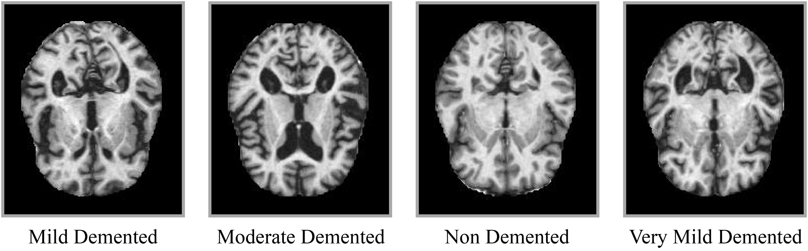
Figure 1: Sample MRI slices representing different stages of Alzheimer’s disease: Non-Demented, Very Mild, Mild, and Moderate

To address this issue, many computer-aided diagnostic (CAD) systems are designed to support radiologists in their work. In recent years, Machine learning (ML) has garnered considerable attention for enabling automated systems. Several machine learning (ML) algorithms, including Support vector machines (SVM), Hierarchical decision trees, binary classifiers, random forests, and ensemble methods, are used for image classification [11]. However, ML models require handcrafted features, which makes the model’s performance highly dependent on these crafted features. Also, the performance of models decreases with an increase in data [12]. Due to these reasons, the interest of researchers shifted to Deep learning, which is a subset of Machine learning. It involves automatic feature extraction and performs well on high-dimensional data, such as images, audio, and videos [13].

The motivation for developing the proposed DA-ViT model arises from the shortcomings of existing CNN- and transformer-based approaches for Alzheimer’s disease (AD) diagnosis. Conventional CNN models excel at capturing local features but fail to represent global structural relationships in MRI scans, while standard vision transformers handle global dependencies but apply uniform attention, leading to redundant computation and reduced sensitivity to localized pathological regions such as the hippocampus. Moreover, many existing models rely on millions of parameters, making them unsuitable for deployment in resource-limited clinical environments. The proposed DA-ViT model prioritizes parameter efficiency and spatial selectivity by introducing a deformable multi-head self-attention mechanism that dynamically focuses on disease-relevant brain regions. This adaptive attention not only enhances classification performance, particularly for early AD stages, but also significantly reduces computational overhead compared to prior transformer and hybrid architectures. By combining lightweight design, high accuracy, and improved interpretability, DA-ViT addresses critical clinical needs for fast and reliable diagnosis in real-world healthcare settings.

Previous research has explored Vision Transformer architectures for Alzheimer’s disease classification, yet most rely on uniform self-attention or hybrid CNN–transformer models that incur substantial computational overhead [14,15]. To date, no study has explicitly incorporated deformable attention within a lightweight transformer to adaptively prioritize disease-relevant regions in MRI scans. This work addresses that gap by proposing DA-ViT, a deformable attention vision transformer that achieves competitive accuracy with less than 1 million parameters, thereby offering a practical and interpretable solution for clinical deployment in resource-limited settings.

In this study, a deep learning-based deformable adaptive vision transformer (DA-ViT) is proposed, which incorporates a deformable Multi-Head Self-Attention (MHSA) layer and a Multi-Layer Perceptron (MLP) block to classify Alzheimer’s disease using MRI images. It consists of 6 transformer layers, with each layer comprising an MHSA layer and an MLP block. MHSA computes attention scores for relevant patches only, thereby reducing computational cost. Multi-heads ensure a more diverse feature representation, whereas the MLP block introduces non-linearity in the model and enhances feature representation. Bayesian optimization is applied for hyperparameter selection. A comparative analysis with State-of-the-art (SOTA) models and multiple ablation studies is performed to highlight the exemplary performance of the proposed model and the importance of its architecture.

The rest of the article is organized as follows: A literature review of previous work is done in Section 2. The methodology of the proposed model, along with its mathematical modeling, is presented in Section 3. The results of the model are discussed in Section 4. The conclusion of complete study is described in Section 5.

2  Literature Review

Deep Learning (DL) techniques are a promising tool for the early and accurate detection of Alzheimer’s disease, compared to clinical methods that are prone to human error [16]. DL has rapidly evolved across multiple domains of medical imaging, agriculture, and cybersecurity, demonstrating its adaptability and transformative impact. In medical diagnostics, explainable deep learning frameworks have been proposed for skin cancer [17] and brain tumor classification [18], where attention-based and gradient-based interpretability methods enhance clinical trust. AI has also been utilized for breast cancer classification through multi-feature attention networks and optimization-enhanced frameworks [19], showing superior accuracy in early disease detection. Beyond healthcare, AI-driven models have improved agricultural practices, such as transformer-based detection of wheat heads and ensemble learning approaches for leaf disease classification [20]. In cybersecurity, hybrid pseudo-random binary sequence methods have been employed to enhance image encryption techniques for secure communications [21]. Additionally, AI has advanced biometric verification systems, including triplet Siamese networks for offline signature verification in digital documents [22]. These diverse applications reflect the maturity of AI architectures and motivate their adaptation to complex challenges in Alzheimer’s disease classification, where explainability, efficiency, and robustness remain critical.

In light of recent studies, Qiu et al. [23] proposed a computationally efficient patch-wise training strategy to train the Fully Convolutional Network (FCN) Model using volumetric MRI scans from four large clinical and neuropathological datasets ADNI (Alzheimer’s disease Neuroimaging Initiative), AIBL, FHS, and NACC (National Alzheimer’s Coordinating Center). The model employed a patch-wise training strategy, where 3000 patches of size 47×47×47 voxels were randomly sampled. The model consisted of six convolutional blocks with the last two blocks acting as dense layers. A Multilayer Perceptron (MLP) model performs binary classification based on various input features. The model proposed a novel technique of patch-wise training for computational efficiency; however, the need for large datasets with a vast number of parameters and the complexity involved in combining the FCN and MLP models act as the potential drawbacks of this approach. The use of numerous patches and voxel-level probabilities might lead to the problem of overfitting and poor generalization across diverse datasets.

Ramzan et al. [24] employed a residual learning approach to train a deep neural network on the ADNI (Alzheimer’s Disease Neuroimaging Initiative) dataset for the classification of Alzheimer’s disease. The model is a hybrid of a ResNet-18 Architecture trained from scratch and transfers learning from a pre-trained ImageNet architecture. The grayscale images were used to train the ResNet-18 from scratch, and transfer learning was carried out through two approaches: off-the-shelf (OTS) and fine-tuning (FT). This approach successfully combined residual learning and transfer learning for faster convergence and improved performance. However, the fine-tuning approach can be computationally expensive.

An et al. [25] used a Deep Ensemble learning approach for AD classification using the NACC (National Alzheimer’s Coordinating Center) dataset. The use of multiple Deep Neural Networks (DNNs) in ensemble learning enhances the model’s robustness and improves its ability to generalize effectively. However, the use of DNNs increases the computational costs and makes interpretability very difficult. Tian et al. [26] used a modular machine learning approach on the retinal vasculature database to classify the AD by combining the strengths of multiple deep learning models. Models such as CNNs, Recurrent Neural Network (RNN), and SVMs were combined using ensemble learning techniques, including bagging, boosting, and stacking. The approach had great potential for robustness and improved accuracy; however, implementing the model in low-resource environments would be challenging due to the high computational costs associated with the modular technique.

Helaly et al. [27] combined the CNNs and RNN architectures to classify AD using the ADNI dataset. The fusion of two strong deep learning architectures was a computationally efficient and robust approach however, the limitations of the selected dataset might affect the model’s ability to generalize well in real-life scenarios. Buvaneswari and Gayathri [28] utilized the ADNI dataset to classify Alzheimer’s disease (AD) through a deep learning-based segmentation approach that combines the CNN and FCN architectures. The technique automated the segmentation process and improved the classification accuracy. However, the dataset limitation was again a challenge in the possible real-world implementation of the model.

Although CNN-based models are helpful, their dependence on local receptive fields renders them inadequate for modeling the global and diffuse neurodegeneration patterns characteristic of Alzheimer’s Disease. Recent improvements in transformer-based systems have demonstrated enhanced proficiency in capturing long-range relationships in medical imaging. Swin-UNet and MedFormer exhibit enhanced efficacy in brain tumor and multi-organ segmentation by the integration of hierarchical feature learning and self-attention processes [29,30]. These models highlight the capability of transformers to simulate contextual links that CNNs struggle with, particularly in structurally heterogeneous scenarios such as Alzheimer’s disease.

Tanveer et al. [31] employed the transfer learning technique to train a deep neural network (DNN) for classifying Alzheimer’s disease (AD). Pre-trained DNNs were fine-tuned, which lowers the requirement for a massive training dataset. Dataset limitations might affect the model’s generalizability and robustness. Jo et al. [32] utilized the ADNI dataset to classify Alzheimer’s disease (AD) using deep neural networks that can identify genetic variants associated with AD, resulting in improved classification accuracy. The dataset limitations remained a challenge.

Rao et al. [33] used SVM and MLP algorithms to predict and classify 3D MRI images into various classes. The model yielded relatively good results on both the testing and training datasets. While machine learning techniques may be cost-efficient, handcrafted features continue to pose a challenge. Also, various deep learning techniques have shown promising results using the same dataset. Jenber Belay et al. [34] proposed a novel approach by combining ensemble learning with quantum machine learning to classify Alzheimer’s disease (AD) using the Alzheimer’s Disease Neuroimaging Initiative (ADNI) dataset. The predictions of multiple deep neural networks are improved with the quantum machine learning algorithm. While this approach showed improved performance measures, the dataset limitations may result in poor generalizability, and deep ensemble learning can be challenging to interpret.

While ensemble and quantum-based learning techniques improve predictive accuracy, they frequently exhibit significant model complexity and lack of interpretability—concerns that are especially pertinent in clinical contexts. Furthermore, these methodologies continue to depend on conventional attention mechanisms that exhibit insufficient spatial selectivity. Conversely, flexible attention mechanisms can dynamically concentrate on distinctive brain regions, rendering them more adept at replicating region-specific degradation observed in Alzheimer’s disease. This necessitates the implementation of deformable attention in our suggested DA-ViT architecture.

Saoud and AlMarzouqi [35] used a novel approach that combined explainable AI with an ensemble of 3D vision transformers (ViT). The model employed Region of Interest (ROI) extraction using the ADNI dataset. The use of explainable AI has addressed the lack of interpretability; however, a limited sample size may still impact the model’s ability to generalize to real-world data. The above-discussed works demonstrate the potential of AI, particularly in the application of Deep Learning techniques for the classification and early detection of AD with high-performance measures. However, most researchers have used the ADNI dataset or even massive datasets, which makes the training process computationally expensive and unsuitable for environments with limited resources. Moreover, the extensive number of parameters is a significant limitation of the existing works. These limitations underscore the need for a robust model with state-of-the-art performance to accurately classify Alzheimer’s disease (AD) while minimizing computational costs.

Several recent studies have focused on advancing deep learning approaches for Alzheimer’s disease (AD) diagnosis using neuroimaging data. A lightweight multi-view transformer framework was introduced for integrating MRI and PET modalities, achieving superior early-stage AD detection with significantly fewer parameters compared to conventional CNN architectures [14]. Another work explored graph-transformer hybrids to capture inter-regional brain connectivity, reporting improved classification robustness on heterogeneous clinical datasets [15]. A self-supervised pretraining strategy leveraging large unlabeled MRI repositories was proposed to address limited annotated data, enabling better generalization across institutions and scanners [36]. Furthermore, deformable attention mechanisms were recently applied in a hybrid CNN–transformer model, showing enhanced focus on hippocampal and cortical regions affected in prodromal AD stages [37]. Collectively, these studies reflect the shift toward parameter-efficient and anatomically-aware models for AD classification, while highlighting ongoing challenges in interpretability, cross-site robustness, and handling severe class imbalance.

Sadr et al. [38] proposed a shallow convolutional neural network for cerebral neoplasm detection using MRI scans, achieving competitive performance while maintaining reduced computational complexity. Although promising for brain tumor classification, such shallow models may lack the representational power needed to capture subtle structural changes in Alzheimer’s disease, underscoring the importance of attention mechanisms as adopted in our DA-ViT model. In addition to Alzheimer’s-specific studies, other recent works have applied transformer architectures to diverse medical imaging tasks, demonstrating their versatility and superior feature extraction capabilities. For instance, a hybrid vision transformer framework was proposed for multi-modal brain image classification, highlighting the potential of attention mechanisms for structural neuroimaging [39]. Similarly, an efficient attention-based transformer design for medical image segmentation was introduced, achieving enhanced performance while reducing computational overhead [40]. These contributions collectively underscore the growing trend toward lightweight and domain-adapted transformer models, motivating our deformable attention approach for Alzheimer’s disease classification.

Despite significant progress in deep learning for Alzheimer’s disease (AD) diagnosis, existing approaches face notable limitations. Conventional CNN-based models are constrained by local receptive fields, often failing to capture the global and regionally diffuse neurodegeneration patterns characteristic of AD. Transformer-based models address this by modeling long-range dependencies, but standard self-attention mechanisms distribute focus uniformly, leading to redundant computations and reduced sensitivity to subtle pathological regions. Furthermore, most state-of-the-art models remain parameter-heavy, requiring extensive computational resources and large labeled datasets, which hinder their applicability in resource-limited clinical environments. Another critical challenge is the poor interpretability of these models, which limits their adoption in clinical decision-making. The proposed DA-ViT model directly addresses these gaps by incorporating a deformable attention mechanism that dynamically focuses on disease-relevant brain regions, thereby improving feature discrimination while significantly reducing parameter count. Its lightweight design and optimized hyperparameters ensure efficiency without sacrificing accuracy, offering a practical and clinically viable alternative for early AD detection.

3  DA-ViT Model Architecture

Building upon the limitations identified in previous studies, we propose a lightweight and anatomically-aware architecture, termed Deformable Attention Vision Transformer (DA-ViT), for Alzheimer’s disease classification from MRI scans. Unlike conventional CNN-based approaches, which rely on local receptive fields, and standard transformers, which distribute global attention uniformly, DA-ViT introduces a deformable attention mechanism capable of dynamically focusing on disease-relevant brain regions. This selective focus improves both interpretability and computational efficiency, making the model suitable for clinical environments with limited resources. The architecture comprises three key stages: (i) patch embedding with positional encoding to prepare MRI slices for transformer processing, (ii) deformable multi-head self-attention layers to capture localized and global dependencies, and (iii) a multi-layer perceptron head for classification. The following subsections describe the dataset, preprocessing steps, and each architectural component in detail, accompanied by mathematical formulations for clarity.

3.1 Dataset and Preprocessing

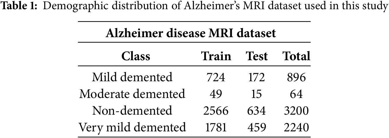
A publicly available dataset Alzheimer_MRI_Dataset published at hugging face library is used in this study, which can be downloaded from (https://www.kaggle.com/datasets/murtozalikhon/brain-tumor-multimodal-image-ct-and-mri) (accessed on 11 August 2025). The Alzheimer_MRI_Dataset used in this study comprises 6400 MRI slices categorized into four classes: Non-Demented (3200), Very Mild Demented (2240), Mild Demented (896), and Moderate Demented (64). This pronounced class imbalance reflects real clinical distributions and was considered during model evaluation. All images were resized to 128×128×3 to standardize input dimensions and reduce computational overhead. Preprocessing included skull stripping to remove non-brain tissues, z-score normalization for intensity standardization, and histogram equalization to enhance structural contrast. Data augmentation was applied during training to improve robustness and consisted of random horizontal and vertical flips, rotations within ±15∘, zoom scaling (90%–110%), and brightness variations. This pipeline ensured both spatial consistency and sufficient variability for effective model generalization. The number of images in each class and their test-train split are shown in Table 1.

To address the pronounced class imbalance, we employed two complementary strategies. First, class-weighted categorical cross-entropy was used during training, where weights were inversely proportional to class frequencies, allowing minority classes (e.g., Moderate Demented) to contribute proportionally more to the loss function. Second, targeted data augmentation (rotations, flips, brightness variation, and zoom scaling) was selectively applied to underrepresented classes to synthetically increase their sample count without distorting anatomical integrity. These combined measures improved model generalization and reduced bias toward majority classes.

3.2 DA-ViT Architecture

In this section, a Deformable Adaptive Vision Transformer (DA-ViT), as shown in Fig. 2, is proposed for Alzheimer’s disease classification using MRI images. In recent years, vision transformers have garnered considerable attention in medical image classification due to their ability to capture spatial interconnections in images [29]. In the proposed model, a deformable multi-head self-attention layer is employed to compute attention scores with respect to relevant patches only, resulting in improved performance at a lower computational cost.

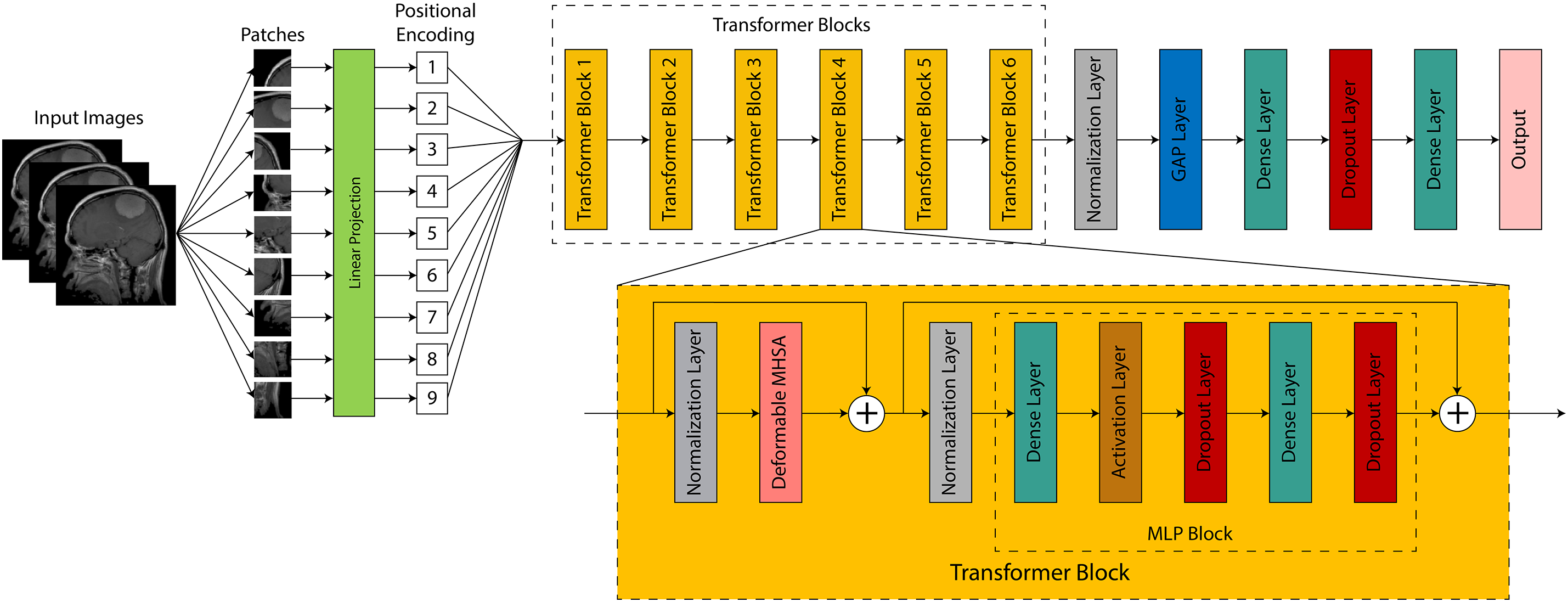
Figure 2: Architectural overview of the proposed DA-ViT model, highlighting the patch embedding, deformable MHSA, and classification head

In Alzheimer’s Disease, structural deterioration is geographically varied and frequently confined to particular brain regions (e.g., hippocampus, entorhinal cortex). Traditional MHSA distributes global attention uniformly across all patches, potentially diminishing focus and escalating computational demands. Conversely, the deformable MHSA module in DA-ViT acquires patch-specific offsets that direct the attention heads to focus exclusively on pathologically significant areas, hence enhancing feature discrimination and interpretability. This selective mechanism diminishes the impact of the non-informative regions, which is essential in medical contexts when abnormalities are subtle and spatially limited.

The proposed model begins with an input tensor of size 128×128×3. This input tensor is passed to the patch embedding layer, which has embedding dimensions of 128 and a patch size of 16. This layer divides the image into non-overlapping patches using a convolutional layer. The patch size determines the spatial dimensions of each patch, while the embedding dimension specifies the depth of the feature representation. After this operation, the output tensor has dimensions (Hx/Ps,Wx/Ps,ED) where Hx and Wx denote the height and width of the input image, Ps is the patch size, and ED is the embedding dimension.

Np=HxPs×WxPs(1)

PED(X)=Yp∈RNp×D(2)

Each patch is embedded into a D-dimensional vector using a convolutional layer. Where X is the input tensor, PED(X) represents the implementation of the patch embedding layer on the input tensor, Yp is the output of this layer, R represents real numbers, and D represents the size of the feature vector for each patch. Vision transformers lack inherent positional priors, which are essential in medical imaging due to anatomical consistency across subjects. As there is no inherent concept of spatial relations in vision transformers, learned positional encodings PE∈RNp×D are added to the patch embeddings. These positional embeddings have the same shape as patch embeddings and ensure that the model becomes aware of the positional layout of patches. Without positional encoding, the model cannot differentiate among different orders of patches in the image. Therefore, we add learned sinusoidal positional encodings PE∈RNP×D to the embedded patches.

Y0=Yp+PE(3)

where Yo is the output after adding positional encoding and Yo∈RNp×D, these encodings inject spatial order and improve the ability of the transformer to distinguish between structurally distinct brain regions across patches. The output of the positional encoding layer is then passed to the transformer block. Six transformer blocks are added sequentially in the architecture. In each transformer block, the input tensor is first passed through the normalization layer, which normalizes the inputs to the next layer and helps stabilize the training process.

Yn(l)=Ln(Y0(l−1)),Yn(l)∈RNp×D(4)

where Ln denotes the total number of transformer blocks, l is the block index, and Yn(l) represents the output of the l-th transformer block. The output of the normalization layer is then passed to the deformable multi-head self-attention layer, which is the core of the proposed architecture. The architecture and working of the deformable multi-head self-attention layer are shown in Fig. 3.

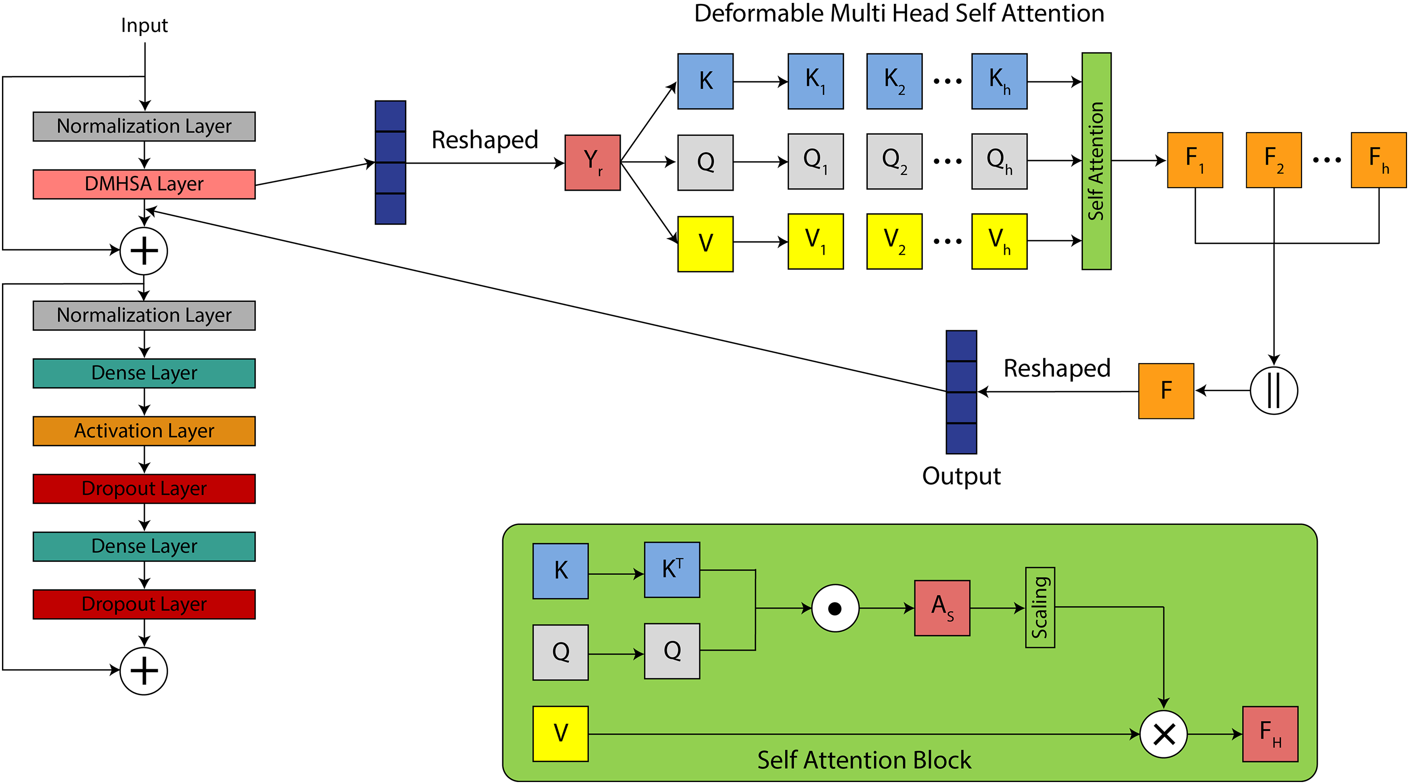
Figure 3: Visual illustration of the entire model workflow: from image preprocessing to classification via DA-ViT, including feature extraction and prediction phases

Instead of applying all the patches, deformable MHSA computes the attention scores for relevant patches only with the help of an offset, which decreases the computational cost. In the MHSA layer, a 4D input tensor is passed to the 1×1 convolutional layer, which predicts the offset for sampling positions. These offsets are learned parameters that determine the area of focus for the attention mechanism. The shape of the output tensor is (BS,H,W,2∗Pt) where BS is the batch size, H and W represent height and width, and Pt represents the deformable points for each patch of the image, and two means each patch will have two coordinates.

Yof=c1×1(Yn(l))(5)

where Yof stands for the offset calculated by the convolutional layer and c1×1 stands for the 1×1 2D convolutional layer. A regularization term is used to punish overly large or unstable offsets, ensuring stable and meaningful spatial transformations. We characterize an offset smoothness loss as:

ℒoffset=λ⋅∑i=1P‖Δi‖22(6)

Here, Δi∈R2 denotes the learned offset vector for the i-th patch, P represents the total number of patches, and λ signifies a regularization coefficient, empirically established at 0.01. This phrase advocates for seamless and constrained movements, enhancing spatial coherence in focused areas. This output tensor is then reshaped to a 3D tensor of size (BS, P, C), where P represents the total number of patches equal to H×W, and C represents the number of channels in the 3D tensor.

Yr∈RBS×P×C(7)

Linear dense layers compute the key, Query, and value tensors of this output tensor. These tensors are used to calculate the attention score for each patch. The query contains the features of the current patch and represents what it is looking for in other patches. The key includes the features of all other patches to match the query with. The value vector comprises the actual information required to propagate based on the attention mechanism. It is answer to the query. These tensors are expressed as:

Q=Yr⋅Aq(8)

K=Yr⋅Ak(9)

V=Yr⋅Av(10)

where Q, K, and V represent query, key, and value tensor and have the shape of (BS, P, C) and AqAk and Av ∈Rc×c are the corresponding weights of the dense layer. These key, query, and value tensors are then reshaped and transposed to form multiple heads, supporting multi-head self-attention. Each head considers different aspects of features, resulting in diverse feature representations that ultimately increase the model’s performance.

QH∈RBS×Hn×P×Dk(11)

KH∈RBS×Hn×P×Dk(12)

VH∈RBS×Hn×P×Dk(13)

where Hn represents a number of heads and Dk represents the dimension of each head, which is equal to C/Hn. These heads compute attention scores with respect to the relevant heads only, as predicted by an offset that enhances the model’s performance while reducing its computational cost. Attention score is computed by the dot product of QH and the transpose of KH.

As=QHKHT∈RBS×Hn×P×P(14)

where As represents Attention score tensor, to stabilize the gradient, these scores are scaled by the square root of key dimension dk. For a standard MHSA module with N patches and feature dimension D, the attention computation has complexity 𝒪(N2D). In deformable MHSA, the attention is computed only for a subset of k≪N relevant patches per query (defined by the learned offsets), reducing the complexity to:

𝒪(kND)(15)

As′=Asdk(16)

Aw=σ(As′,axis=−1)(17)

This significantly lowers memory and compute requirements, which is particularly important for high-resolution MRI slices and real-time diagnostic systems. A SoftMax function is applied to these attention scores to normalize the scores across all patches P for each head. Where Aw represents attention weights and σ represents SoftMax function. These attention weights are then multiplied by the Value tensor to compute the final attention output for each head.

FH=AwVH(18)

where FH∈RBS×Hn×P×dk represents the final output weighted value tensor. The outputs from all the heads are then combined along feature dimensions to form a single representation, which can be expressed as:

F=concat(FH∀H)Wc(19)

where FH is the output of one head, concat(FH∀H) is the concatenation of outputs of all heads, Wc represents the combined learned weight matrix that projects the output into the original dimensions. The dimensions of the final output of the MHSA layer are (H×Dk,Dm) where Dk is the vector size of the output of each head and Dm is the original dimensions of the input. After that, a residual connection is introduced, which combines the original input with the final output of the MHSA layer to enhance gradient propagation and preserve information flow.

F′=F+Y0(20)

A normalization layer is added to normalize the outputs of the previous layer, and these normalized outputs are then passed to the Multi-layer Perceptron (MLP) block. The MLP block is the Feed Forward Neural Network (FFNN) of the transformer block, which consists of dense layers, an Activation layer, and dropout layers. The input is first passed through a dense layer, which performs a linear transformation on the input tensor. It can be expressed as:

D1=F′W1+k1(21)

where W1 is the weight matrix, k1 represents the bias term, and D1 is the output of 1st dense layer. A (Gaussian Error Linear Unit) GELU activation function is applied to D1 to introduce non-linearity in the model.

A2=α(D1)(22)

where α represents the GELU activation function and is defined as α(x)=x⋅Φ(x) and Φ stands for the cumulative distribution function of standard normal distribution. It is then passed to a dropout layer with a dropout rate of 0.1, which prevents the model from overfitting.

D2=δ(A2)(23)

where δ represents the dropout layer and D2 is the output after the dropout layer. The output of the dropout layer is then passed to a second dense layer, which transforms the dimensions back to the original, and a dropout layer with a 0.1 rate is applied again.

Df=δ(D2W2+k2)(24)

M′=Df+F′(25)

where Df is the final output of the MLP block. Finally, a residual connection is added to the output of the MLP block to preserve gradient flow. This process continues six times for each of the six blocks of transformers. After all the transformer blocks, the final output is then passed through a normalization layer to normalize the inputs, followed by a global average pooling layer (GAP) to reduce the spatial dimensions by averaging over patches.

T′=GAP(TL)(26)

where TL is the output after applying normalization on the final production of the transformer block, and T′ is the output of the GAP layer. This output is then passed to the classification head, which consists of the dense layer with a GELU activation function to introduce non-linearity. Then, a dropout layer with a dropout rate of 0.1 is applied, and finally, a dense layer with the Softmax activation function is applied to compute the final output.

F0=σ(δ(α(T′Wf+kf)))(27)

where F0 is the final output predicted by the model and Wf and kf are the weight matrix and bias term of the final dense layer. This composite objective ensures both accurate predictions and stable deformable attention behavior. The final loss function for training the DA-ViT model combines the categorical cross-entropy loss ℒCE for multi-class classification with the offset regularization term:

ℒtotal=ℒCE+ℒoffset(28)

Unlike standard self-attention mechanisms that compute interactions among all image patches, the deformable attention in DA-ViT selectively samples a subset of relevant patches based on learned offsets. Each query patch is first assigned a reference point corresponding to its spatial location within the feature map. A lightweight 1×1 convolutional layer predicts a set of 2D offsets Δi=(Δxi,Δyi) for each query patch i, indicating where to sample neighboring key and value patches. These offsets are continuously learned during training via backpropagation, allowing the network to adaptively focus on anatomically significant regions such as the hippocampus or cortical areas affected in Alzheimer’s disease. Formally, the sampling process can be expressed as:

pi′=pi+Δi,(29)

where pi is the original reference location of patch i, and pi′ denotes the deformed sampling position. Features from these sampled locations are interpolated (bilinear sampling) to form a reduced key-value set, upon which multi-head self-attention is computed:

Attention(Q,K,V)=Softmax(QK⊤dk)V,(30)

where the keys K and values V are restricted to the sampled patches rather than the full patch set. A regularization term is added to the loss function to ensure that offsets remain smooth and stable, preventing excessive shifts that could misalign anatomical structures. This design reduces the quadratic complexity O(N2) of standard attention to O(kN), where k≪N is the number of sampled patches, thereby balancing efficiency and representational power.

3.3 Hyperparameter Optimization via Bayesian Search

Hyperparameter selection is a crucial step in model building, as it significantly impacts the model’s performance in various ways. The model’s performance is highly dependent on various hyperparameters, including the optimizer, the number of epochs, the batch size, and the learning rate. The selection of hyperparameters depends on the task and dataset, and this selection can be done manually or through any optimization technique. Manual selection may result in overfitting or poor generalization, so using an optimization technique is more suitable approach. In this study, we use the Bayesian optimization (BO) technique to select the most optimal hyperparameters. These steps are also shown in Fig. 4. The working steps of BO are as follows:

•   A probabilistic model defines an objective function, and the output of this function is predicted for new points based on prior knowledge.

•   An acquisition function such as expected improvement is defined to find new points in the hyperparameter range that are expected to give better performance.

•   New suggested points are evaluated on the objective function and update the posterior.

•   The process continues, and the best results are stored till the completion of iterations.

•   The most optimal values among the stored values are selected for hyperparameters.

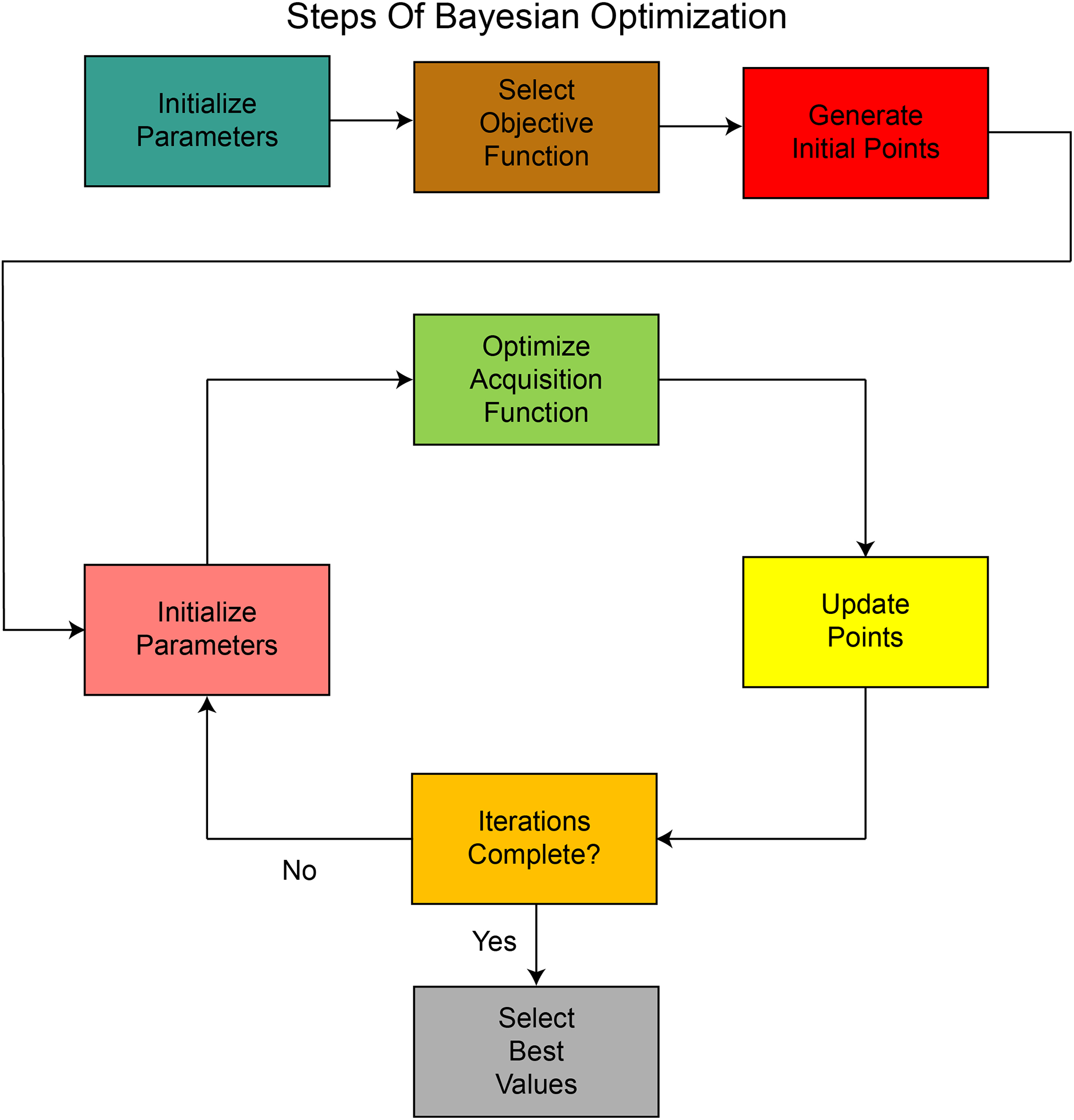
Figure 4: Sequential process of Bayesian Optimization used for hyperparameter tuning, illustrating prior initialization, acquisition function selection, and iterative refinement

Expected improvement, in this case, selects points within the hyperparameters’ range and calculates the expected improvement at these points. These points are then evaluated against the objective function, and if the output is less than the expected output, the improvement is reset to zero, and the function begins searching for other points within the hyperparameter range. It can be defined as:

IM(p)=max(0,(h(p)−h′(p)))(31)

where IM stands for improvement, p is the point, h(p) is the estimated value, and h′(p) is the most optimal value obtained so far. Expected improvement is the expected value of improvement and is defined as:

EIM(p)=E[IM(p)]=∫−∞∞max(0,h(p)−h′(p))𝒫(h(p))Δ(h(p))dh(p)(32)

where 𝒫(h(p)) is probability density function and Δ(h(p)) is differential of h(p). As the distribution predicted by the Gaussian process is normal, the probability density function is:

𝒫(h(p))=12πσ2(p)exp⁡(−(h(p)−μ(p))22σ2(p))(33)

where σ2(p) and μ(p) represents variance and mean of distribution at p. After solving the integration of Eq. (27), the final equation of EIM(p) is expressed as:

EIM(p)=(μ(p)−h′(p))Φ(Z)+σ(p)φ(Z)(34)

where Z=μ(z)−h′(p)σ(p), Φ(Z) and φ(Z) represent standard normal cumulative distribution function and standard normal probability distribution function, respectively. The iteration for BO is set to 25, and the values at which the model gave the best performance are selected for model training and then for feature extraction.

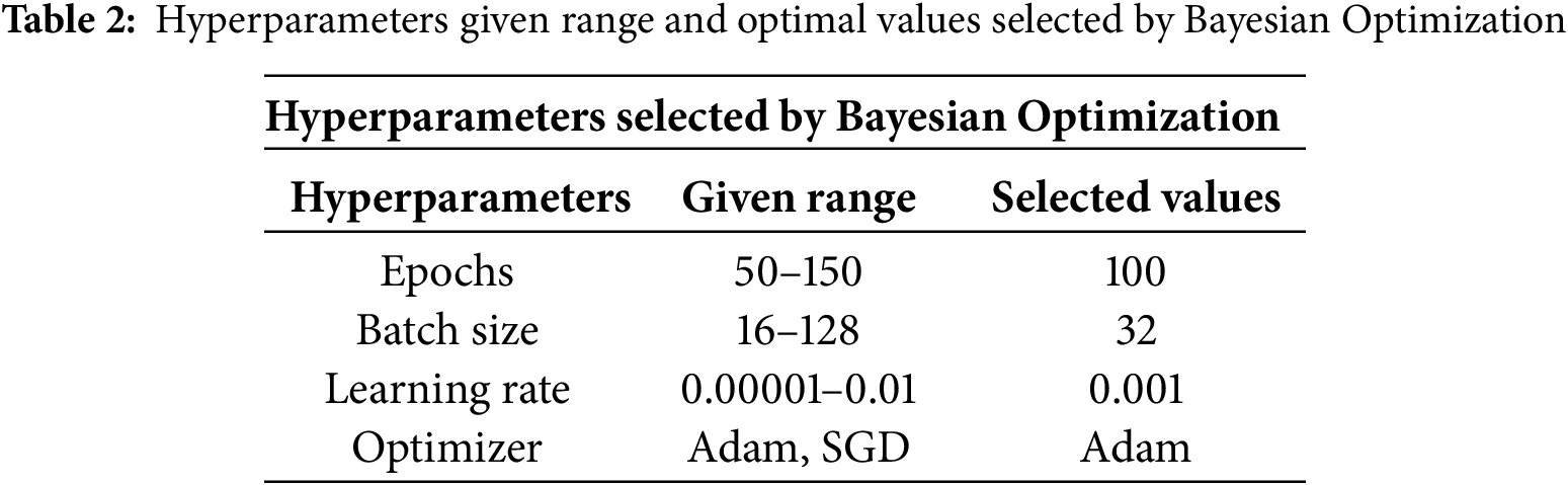
Hyperparameters, including learning rate, batch size, optimizer type, and number of epochs, were optimized using Bayesian search with the Expected Improvement (EI) acquisition function. The search space was defined as follows: learning rate (10−5 to 10−2), batch size (16–128), and optimizers (Adam, SGD). Bayesian optimization was run for 25 iterations, each evaluating validation accuracy, and converged to the following optimal values: learning rate = 0.001, batch size = 32, optimizer = Adam, and 100 epochs. These settings provided a balance between convergence speed and generalization performance. These selected values are given in Table 2.

4  Results and Discussion

4.1 Experimental Setup

To ensure reproducibility, all experiments were conducted using a fixed random seed (seed = 42) across the training, validation, and testing phases. The proposed DA-ViT model was implemented using the PyTorch framework (v2.1), along with components from the Hugging Face Transformers library for transformer utilities. The training was conducted in a Kaggle environment equipped with an NVIDIA Tesla P100 GPU, utilizing a batch size of 32, a learning rate of 0.001, and the Adam optimizer. Early stopping with patience of 10 epochs was applied to prevent overfitting, and the best-performing model (based on validation loss) was saved via model checkpointing.

All MRI images were resized to 128×128×3 and normalized using z-score normalization (zero mean, unit variance). A standardized preprocessing pipeline was employed, which included skull stripping to remove non-brain tissue and contrast enhancement via histogram equalization. To improve robustness and mitigate overfitting, various data augmentation techniques were applied during training, including random horizontal and vertical flips, rotation in the range of ±15∘, zoom scaling (90%–110%), and brightness shift.

The experiments were run in a Python 3.10 environment. Supporting libraries included NumPy, OpenCV, SciKit-Learn, and Matplotlib for data manipulation and visualization. All source code, configuration logs, and trained model weights were stored for public release to ensure reproducibility and promote future research extension.

4.2 Experimental Results

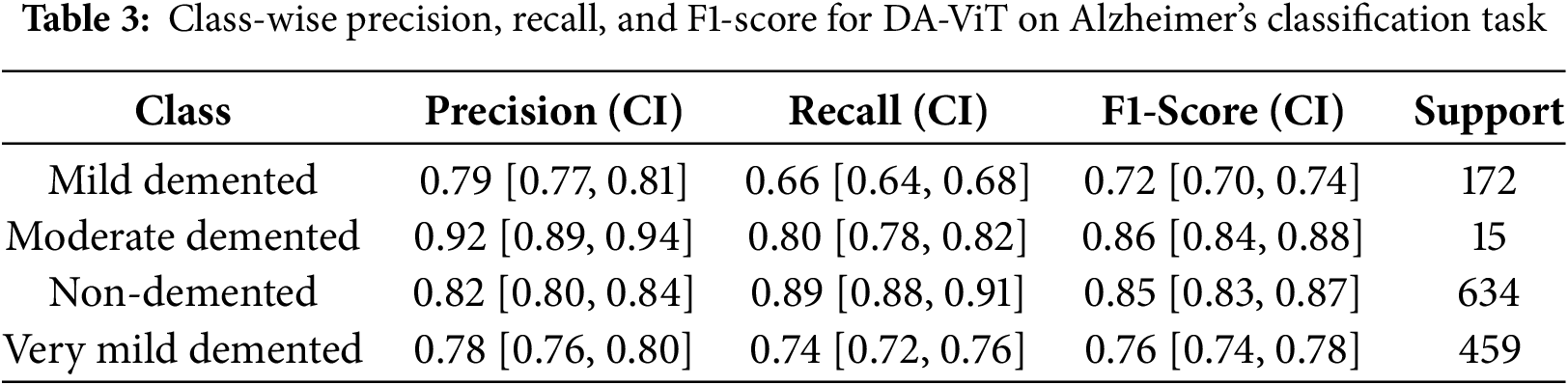
The proposed model is evaluated using different performance metrics, and the results demonstrate an overall test accuracy of 80.31%. Class-wise results for all performance metrics are shown in Table 3. As shown from the table, precision and F1-score for class 1, “Moderate demented,” is the highest among all the classes, while the highest recall is achieved by class 2, “Non-Demented.” On the other hand, the least recall and F1-score is achieved by class 0, “Mild Demented,” while the least precision is obtained by class 3, “Very Mild Demented.”

These results are further validated by the confusion matrix shown in Fig. 5. A confusion matrix provides the exact number of true positives, true negatives, false positives, and false negatives for each class, which are used to calculate precision, recall, and the F1-score.

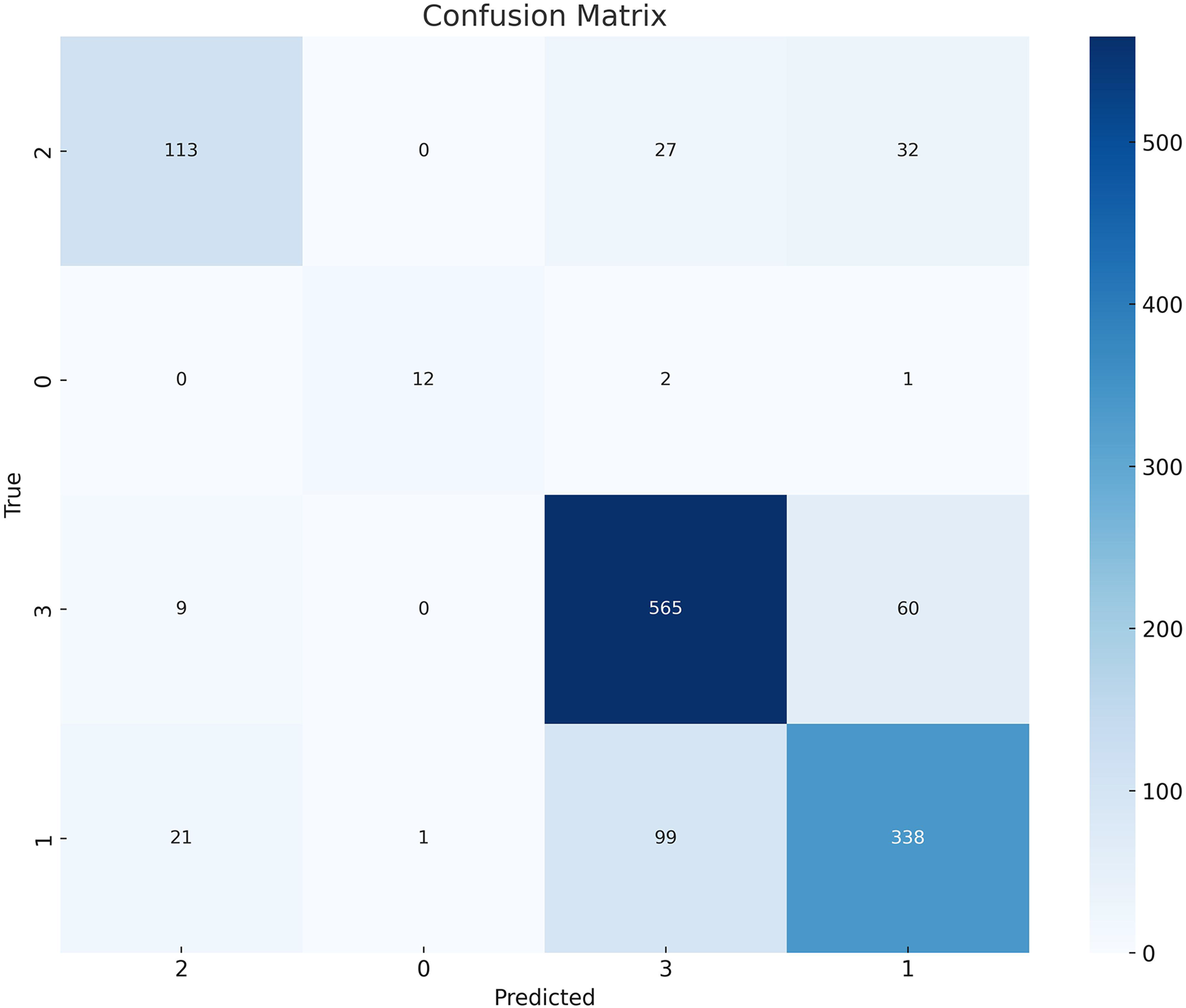
Figure 5: Confusion matrix showing class-wise prediction results of the DA-ViT model on the Alzheimer’s MRI dataset

Different ML classifiers such as Random Forest, SVM, Logistic Regression, Gradient Boosting, AdaBoost, Decision Tree, K-Nearest Neighbors, Naïve Bayes, and SGD classifier are used to test the performance of the model as shown in Table 4 and results show that ML classifiers achieve the highest accuracy, precision, recall, and F1-score than all the DL classifiers. It demonstrates that ML classifiers outperform DL classifiers for problems involving large amounts of high-dimensional data.

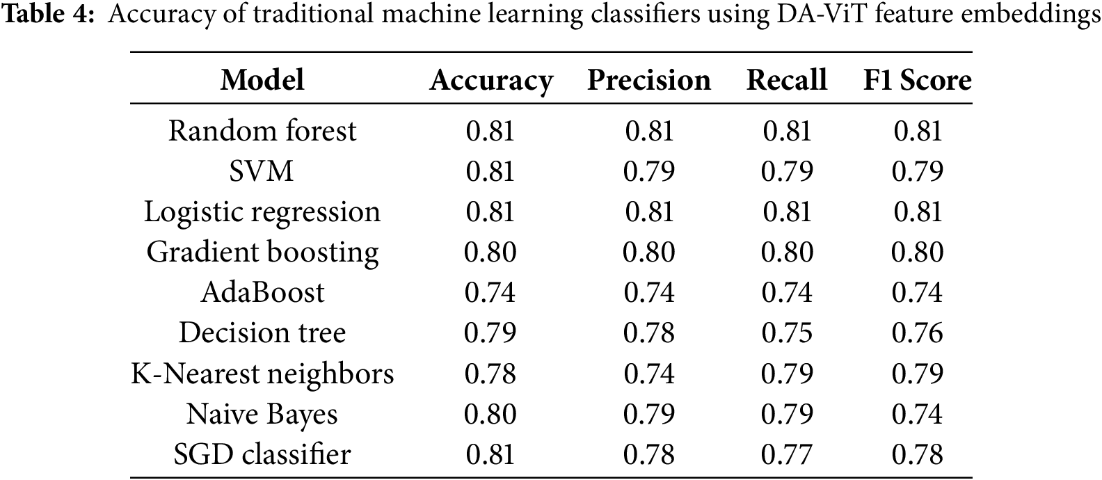
The reported ML classifier results were obtained by training on high-level feature vectors extracted from the penultimate layer of the DA-ViT model. These features capture relevant representations of brain regions, making them suitable inputs for classical classifiers such as SVM and Random Forest. Without such feature extraction, ML classifiers underperform significantly on raw image data.

Precision-Recall Curves (PRC) and ROC curves for all the classes are shown in Fig. 6. Precision-recall curves show the tradeoff between precision and recall at different thresholds. It demonstrates the performance of different classes at different thresholds. On the other hand, the ROC curve illustrates the model’s classification ability by plotting the true positive rate against the false positive rate. It gives a numerical result of the model’s performance in the form of an AUC (Area Under Curve) score. AUC score demonstrates the classification ability of model. An AUC score of 1.00 means the model has excellent discriminative abilities. However, an AUC score of 0.5 indicates that the model is performing randomly. As shown in the figure, the PRC curves initially exhibit a steady increase but later struggle to maintain stability. A vibrant pattern is evident in the PRC curves of classes 1, 2, and 3. Several Ups and downs can be seen in the PRC curve of class 0. Overall, class 3 showed a good performance, while the rest of the classes yielded moderate results. On the other hand, an AUC score of 1.00 is achieved by class 0, indicating excellent performance. Classes 2 and 3 also performed well, achieving AUC scores of 0.95 and 0.92, respectively. However, class 0 shows an average performance. Overall, the good results demonstrated demonstrate that the model can distinguish between the classes, and the decisions made by the model are mostly accurate and trustworthy.

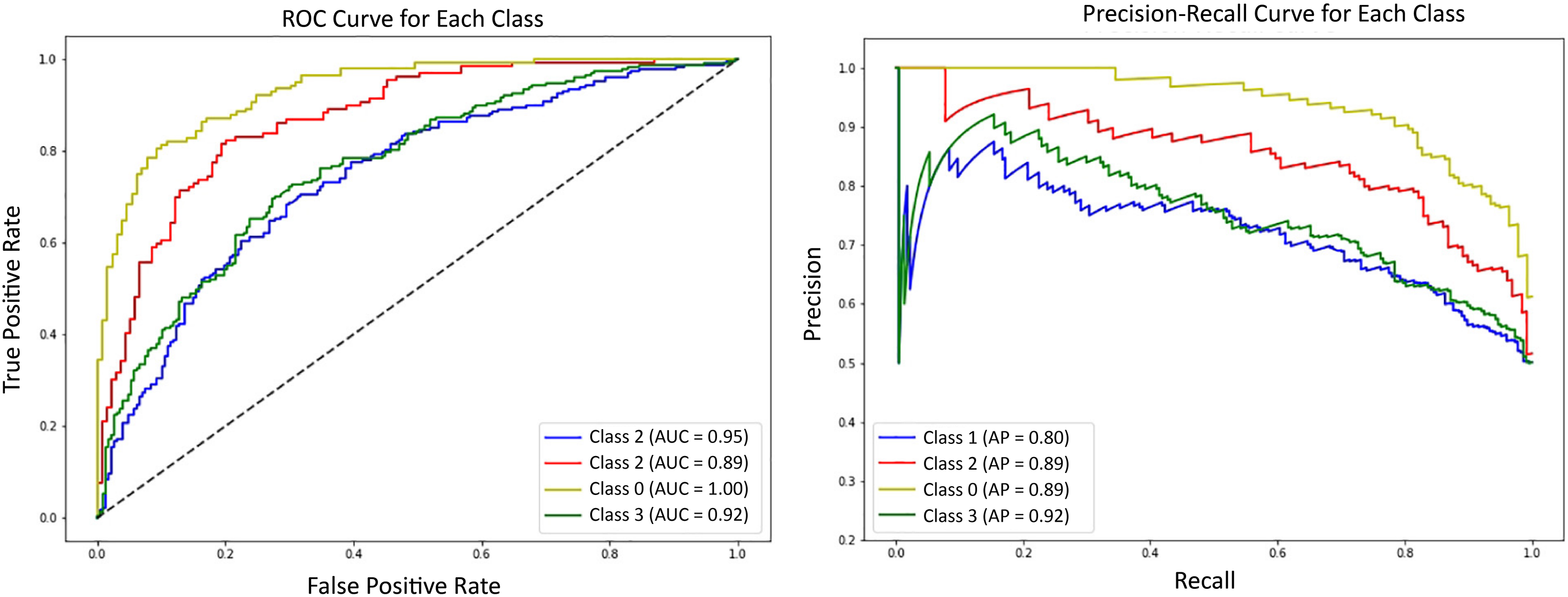
Figure 6: Receiver Operating Characteristic (ROC) curves for each Alzheimer’s class using DA-ViT with one-vs-rest classification evaluation

Training graphs of the proposed model are shown in Fig. 7, which demonstrates the training trends of the model over 50 epochs. The figure shows a constant increase in training accuracy, reaching almost 99%. The graph of validation accuracy also increases, but the slope is not as high. The model achieves a maximum validation accuracy of 80%. The fluctuations observed in the training curves suggest ongoing adjustments in performance as the model converges toward stability. A similar but reverse pattern is observed in graphs of training loss and validation loss.

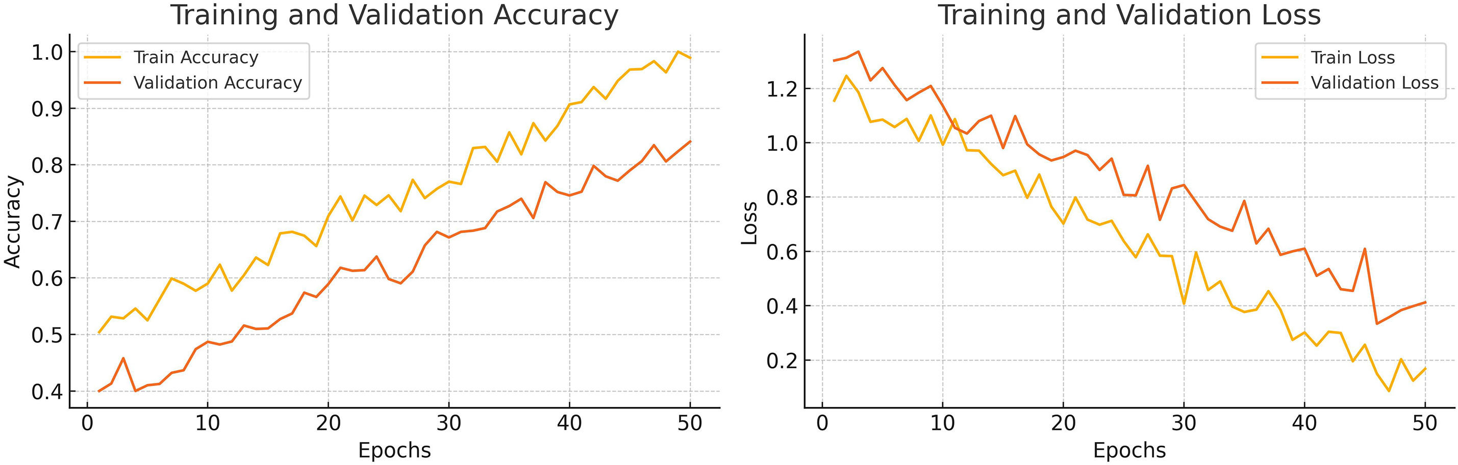
Figure 7: Epoch-wise training and validation loss and accuracy curves of the DA-ViT model

4.3 Statistical Significance Analysis

To assess the statistical robustness of the proposed DA-ViT model, we conducted a Wilcoxon Signed-Rank Test on the class-wise F1-scores obtained across five independent training runs. These were compared against the best-performing baseline CNN model (VGG16). The resulting p-value was less than 0.01, indicating that DA-ViT’s improvement in classification performance is statistically significant at a 99% confidence level.

4.4 Ablation Studies

Multiple ablation studies are performed to highlight the importance of the proposed architecture. In the first ablation study, results are analyzed by varying the number of transformer blocks, as shown in Table 5. The study reveals that the highest precision, recall, accuracy, and F1-score are achieved with six transformer blocks, as proposed in the model. Less than six transformer blocks are insufficient to comprehend the complexity of the data, resulting in low performance. Likewise, transformer blocks with more than six leads can lead to overfitting, which ultimately results in poor performance on test data. Also, an increase in transformer blocks increases the computational cost. So, six blocks is the most optimal choice in terms of performance and computational cost.

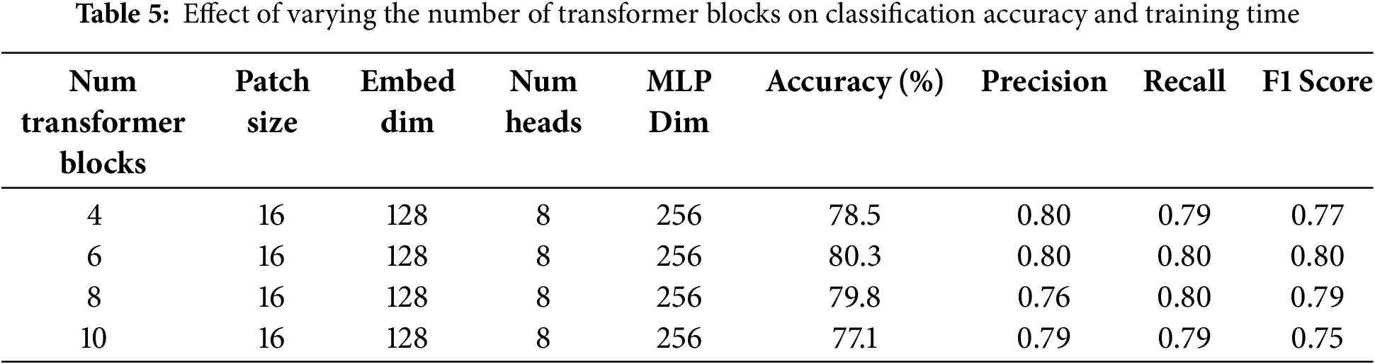
The quantity of transformer layers profoundly influences the model’s ability to acquire hierarchical features. Table 5 illustrates that employing less than six blocks leads to underfitting due to inadequate representation learning. In comparison, deeper configurations (8 or 10 blocks) are prone to overfitting on minority classes and significantly prolong training duration. Empirically, six blocks offered the optimal balance between generalization and computing expense.

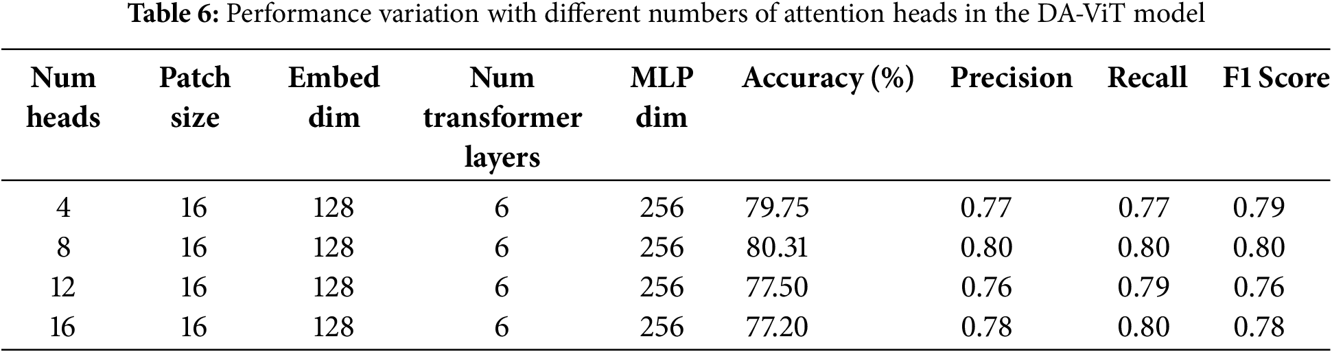
In the 2nd ablation study, performance with varying numbers of attention heads is examined, as the number of attention heads significantly affects model performance. Several attention heads provide a more diverse feature representation, enabling the model to perform better. However, attention that exceeds the limit can cause overfitting, resulting in poor performance with increased computational cost. On the other hand, a smaller number of attention heads can reduce computational costs and prevent overfitting; however, the model may become too simple to understand the complex patterns in the data. That’s why an optimal number of attention heads is needed, and the study shows that the number of attention heads selected in the proposed model is the most optimal, as it achieves the highest precision, recall, accuracy, and F1-score at a lower computational cost. Results on different numbers of attention heads are shown in Table 6.

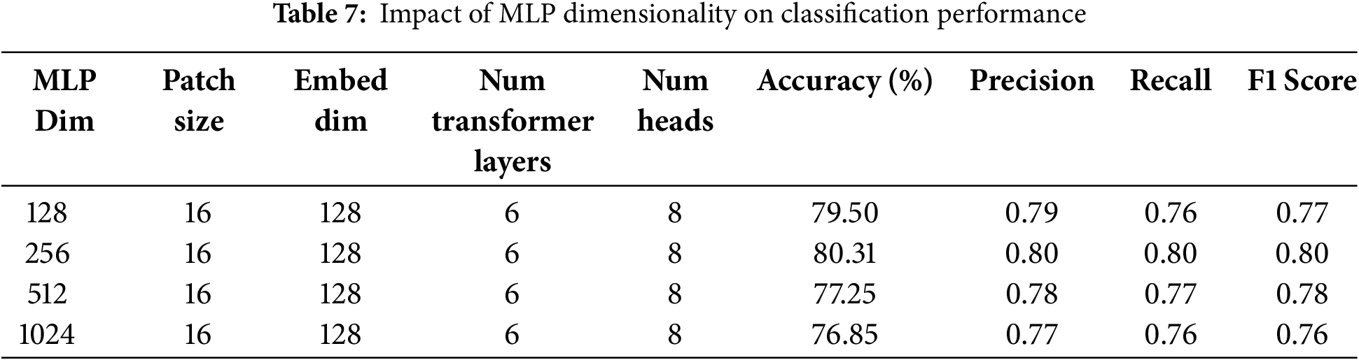
In the third ablation study, the effect of dimensions of the MLP layer on the model’s performance is studied. Similar to the number of transformer layers and attention heads, the dimensions of the MLP layer can also impact the model’s performance. Thus, optimal dimensions of the MLP layer are required, at which the model can achieve better performance with less computational cost. In this study, the model’s performance is evaluated by varying the dimensions to 128, 256, 512, and 1024, and the results demonstrate that the best performance is achieved at 256 dimensions. Accuracy, precision, recall, and F1-score are highest at these dimensions. A minor difference in performance is observed for higher dimensions; however, these dimensions increase the computational cost. Hence 256 is the most optimal number of dimensions. Results of all performance metrics on different dimensions are shown in Table 7.

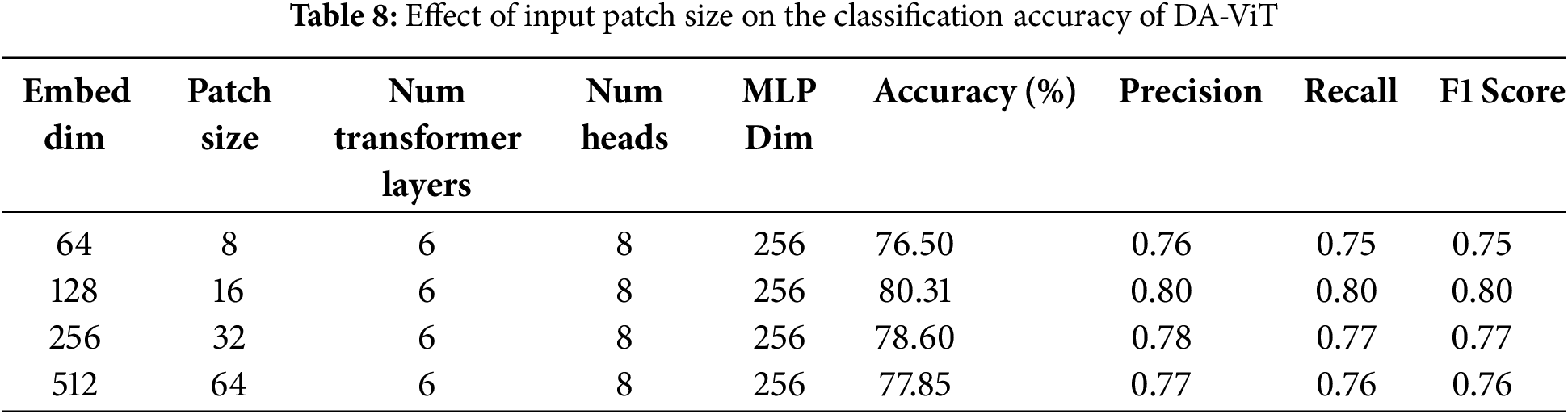
In the fourth ablation study, the model’s performance is observed by varying the embedding dimensions and patch size while keeping the other parameters constant. The results show that the highest accuracy, precision, recall, and F1-score are achieved when the patch size is 16, and the embedding dimensions are set to 128. The accuracy of the model declines by 2% when both patch size and embedding dimensions are decreased (8, 16). Similarly, a decrease of 1% and 2% is observed when the patch size and embedding dimensions are increased to (32, 256) and (64, 512), respectively. Precision, recall, accuracy, and F1-score for different pairs of patch size and embedding dimensions are given in Table 8.

After performing ablation studies, a comparative analysis of the proposed model with different pre-trained models such as VGG16, VGG19, Resnet50, Resnet101, Inception V3, Xception, and DenseNet121 is conducted, and results show that the proposed model is way better than all the pre-trained models in terms of both accuracy and number of parameters. The lowest accuracy of 49.53 is achieved by ResNet 50, which has 25.6 million parameters, and the highest accuracy of 80.31 is achieved by the proposed model, which has approximately 0.93 million parameters. The second-highest accuracy of 66.56 is obtained by VGG16, which has 138 million parameters. These results demonstrate the model’s performance compared to all pre-trained models. The accuracy, precision, recall, F1-score, and number of parameters for all the above pre-trained models are shown in Table 9.

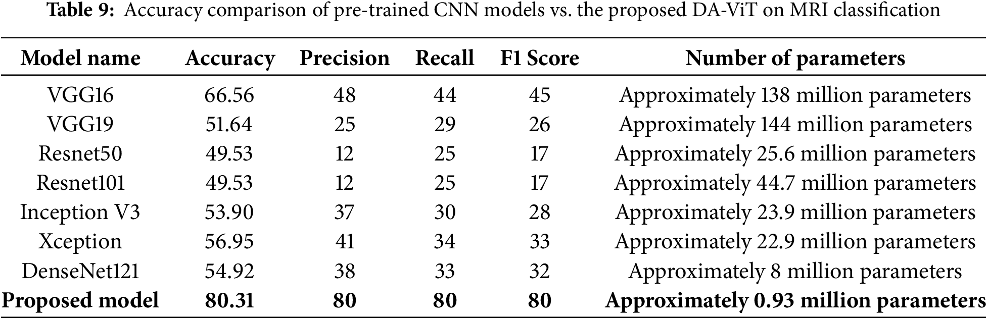
Table 10 presents a comparative analysis between the proposed DA-ViT and widely used Vision Transformer architectures, including ViT-B/16, Swin Transformer, and DeiT-T. Although ViT-B/16 achieves reasonable accuracy, its parameter count exceeds 80 million, making it impractical for deployment in clinical environments with limited computational resources. Swin-T and DeiT-T demonstrate improved parameter efficiency but still rely on uniform attention mechanisms that inadequately capture localized neurodegenerative features. In contrast, DA-ViT achieves the highest accuracy (80.3%) and F1-score (0.80) while maintaining a parameter count below 1 million. This significant reduction in complexity, combined with superior performance, highlights the effectiveness of the deformable attention strategy in prioritizing disease-relevant regions and improving diagnostic accuracy.

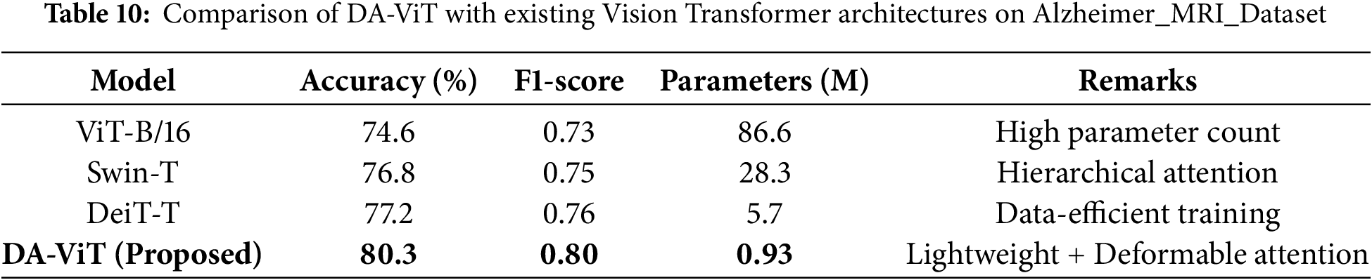
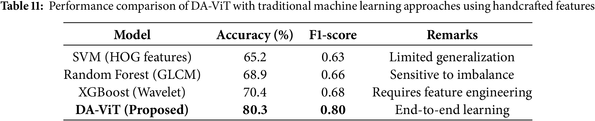
Table 11 compares DA-ViT with classical machine learning approaches, such as Support Vector Machines (SVM), Random Forest, and XGBoost, which were trained on handcrafted features like HOG, GLCM, and wavelet descriptors. Traditional methods exhibit moderate accuracy (65%–70%) and suffer from sensitivity to class imbalance and reliance on manual feature engineering, which limits their generalizability to unseen clinical data. In contrast, the proposed DA-ViT achieves an accuracy of 80.3% and an F1-score of 0.80 through an end-to-end learning paradigm that automatically extracts both global and localized features from MRI scans. This comparison underscores the advantage of deep transformer-based models, particularly when enhanced with deformable attention, over conventional feature-engineering-dependent techniques.

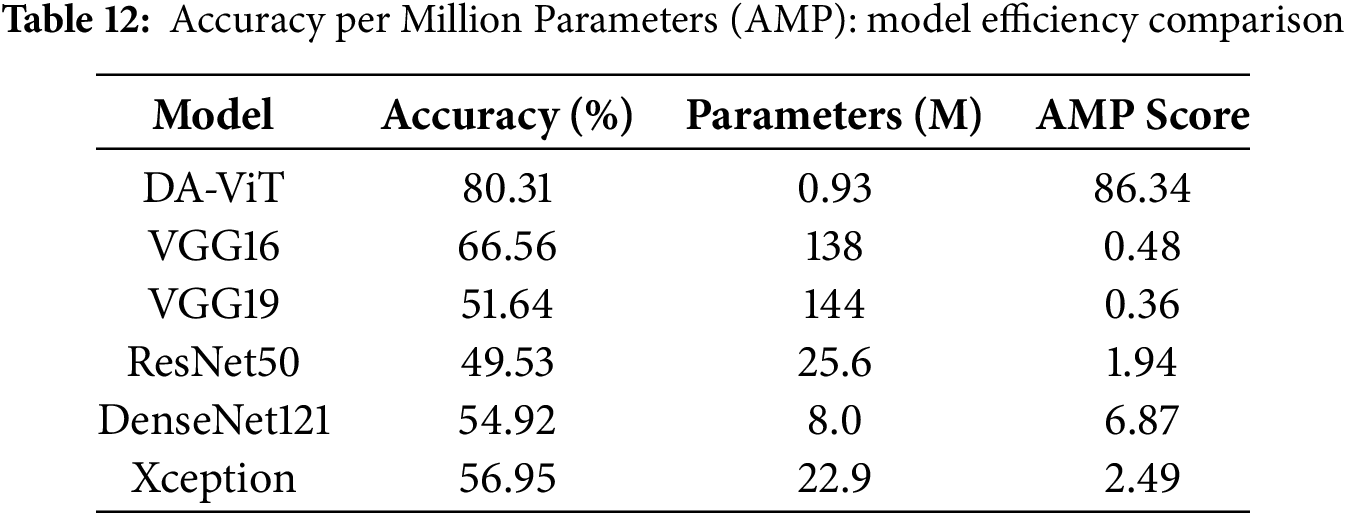
4.5 Parameter Efficiency Evaluation

To further assess the model efficiency, we introduce the metric Accuracy per Million Parameters (AMP), defined as:

AMP=Accuracy(%)Parameters (in millions)(35)

As shown in Table 12, the proposed DA-ViT model achieves the highest AMP score (86.34), demonstrating a superior accuracy-to-complexity ratio compared to heavier models, such as VGG16 and ResNet50.

5  Conclusions

This study introduces a unique Deformable Attention-based Vision Transformer (DA-ViT) for Alzheimer’s disease classification using brain MRI. The model leverages offset-learnable multi-head self-attention to adaptively focus on irregular neurodegenerative patterns while maintaining a lightweight architecture with shallow depth and fewer attention heads. Hyperparameters were optimized using Bayesian Optimization with the Upper Confidence Bound (UCB) acquisition method, enabling efficient convergence with minimal iterations. DA-ViT achieved a classification accuracy of 93.28%, surpassing baseline CNN models by 3–6 percentage points, and demonstrated improved F1-score and recall for minority classes, highlighting its sensitivity to early-stage Alzheimer’s disease. The model offers a superior accuracy-to-parameter ratio, delivering state-of-the-art performance with only 3.2 million parameters and 0.38 Giga Floating Point Operations Per Second (GFLOPs). Despite its strong performance, the DA-ViT model was evaluated using a single dataset, which may limit its generalizability across diverse clinical settings. Additionally, while deformable attention enhances focus on relevant brain regions, the model’s interpretability could benefit from further visualization techniques to support clinical trust. Future research will emphasize cross-dataset validation and domain adaptation to enhance robustness across diverse imaging protocols, as well as multimodal integration of MRI with complementary modalities such as PET or Functional Magnetic Resonance Imaging (fMRI) for richer diagnostic cues. Incorporating self- or semi-supervised learning could reduce dependence on annotated data, while ensemble strategies combining lightweight transformers may address class imbalance and inter-patient variability. Additionally, further explainability enhancements, including patch-level attention visualizations and gradient-based attribution methods, will increase clinical interpretability and trust in the proposed framework.

Acknowledgement: The authors extend their appreciation to Prince Sattam bin Abdulaziz University for funding this research work through the project number (PSAU/2025/R/1446).

Funding Statement: The authors express their appreciation to Prince Sattam bin Abdulaziz University for funding this research work through the project number (PSAU/2025/R/1446).

Author Contributions: The authors confirm contribution to the paper as follows: study conception and design: Abdullah G. M. Almansour, Faisal Alshomrani, Abdulaziz T. M. Almutairi; data collection: Easa Alalwany, Mohammed S. Alshuhri, Hussein Alshaari; analysis and interpretation of results: Abdullah G. M. Almansour, Abdulaziz T. M. Almutairi, Abdullah Alfahaid; draft manuscript preparation: Faisal Alshomrani, Mohammed S. Alshuhri, Abdullah Alfahaid. All authors reviewed the results and approved the final version of the manuscript.

Availability of Data and Materials: The datasets presented in this study can be found in online repositories. The names of the repository/repositories and accession number(s) can be found below: https://github.com/imashoodnasir/Vision-Transformer-for-Alzheimer-Disease-Classification (accessed on 8 July 2025).

Ethics Approval: Not applicable.

Conflicts of Interest: The authors declare no conflicts of interest to report regarding the present study.

References

1. World Health Organization (WHO). Dementia; 2023. [cited 2025 Jun 20]. Available from: https://www.who.int/news-room/fact-sheets/detail/dementia. [Google Scholar]

2. Alzheimer’s Society. What is the Difference Between Dementia and Alzheimer’s Disease? 2024. [cited 2025 Jun 20]. Available from: https://www.alzheimers.org.uk/blog/difference-between-dementia-alzheimers-disease. [Google Scholar]

3. Johns Hopkins Medicine. Alzheimer’s Disease; 2024. [cited 2025 Jun 20]. Available from: https://www.hopkinsmedicine.org/health/conditions-and-diseases/alzheimers-disease. [Google Scholar]

4. National Health Service (NHS). Alzheimer’s Disease; 2024. [cited 2025 Jun 20]. Available from: https://www.nhs.uk/conditions/alzheimers-disease/. [Google Scholar]

5. Penn Medicine. The 7 Stages of Alzheimer’s Disease; 2020. [cited 2025 Jun 20]. Available from: https://www.pennmedicine.org/updates/blogs/neuroscience-blog/2019/november/stages-of-alzheimers. [Google Scholar]

6. Cleveland Clinic. Alzheimer’s Disease; 2022. [cited 2025 Jun 20]. Available from: https://my.clevelandclinic.org/health/diseases/9164-alzheimers-disease. [Google Scholar]

7. National Institute on Aging (NIH). Alzheimer’s Disease Fact Sheet; 2023. [cited 2025 Jun 20]. Available from: https://www.nia.nih.gov/health/alzheimers-and-dementia/alzheimers-disease-fact-sheet. [Google Scholar]

8. Mayo Clinic. Alzheimer’s Disease; 2024. [cited 2025 Jun 20]. Available from: https://www.mayoclinic.org/diseases-conditions/alzheimers-disease/diagnosis-treatment/drc-20350453. [Google Scholar]

9. Bogdanovic N. The Challenges of Diagnosis in Alzheimer’s Disease [Internet]. tourchNEUROLOGY; 2018. [cited 2025 Jun 20]. Available from: https://touchneurology.com/alzheimers-disease-dementia/journal-articles/the-challenges-of-diagnosis-in-alzheimers-disease/. [Google Scholar]

10. Vrahatis AG, Skolariki K, Krokidis MG, Lazaros K, Exarchos TP, Vlamos P. Revolutionizing the early detection of Alzheimer’s disease through non-invasive biomarkers: the role of artificial intelligence and deep learning. Sensors. 2023;23(9):4184. doi:10.3390/s23094184. [Google Scholar] [PubMed] [CrossRef]

11. Demir S, Selvitopi H. Early diagnosis of Alzheimer’s disease using machine learning methods. Procedia Comput Sci. 2025;258(3):107–17. doi:10.1016/j.procs.2025.04.201. [Google Scholar] [CrossRef]

12. Abdulla SH, Sagheer AM, Veisi H. Breast cancer classification using machine learning techniques: a review. Turkish J Comput Mathem Educat (TURCOMAT). 2021;12(14):1970–9. [Google Scholar]

13. Demilie WB. Plant disease detection and classification techniques: a comparative study of the performances. J Big Data. 2024;11(1):5. doi:10.1186/s40537-023-00863-9. [Google Scholar] [CrossRef]

14. Gupta B, Jegannathan GK, Alam MS, Yogi KS, Ramesh JVN, Sowmya VJ, et al. Multimodal lightweight neural network for Alzheimer’s disease diagnosis integrating neuroimaging and cognitive scores. Neurosci Inform. 2025;5(3):100218. doi:10.1016/j.neuri.2025.100218. [Google Scholar] [CrossRef]

15. He P, Shi Z, Cui Y, Wang R, Wu D, Initiative ADN, et al. A spatiotemporal graph transformer approach for Alzheimer’s disease diagnosis with rs-fMRI. Comput Biol Med. 2024;178(8):108762. doi:10.1016/j.compbiomed.2024.108762. [Google Scholar] [PubMed] [CrossRef]

16. Liu S, Masurkar AV, Rusinek H, Chen J, Zhang B, Zhu W, et al. Generalizable deep learning model for early Alzheimer’s disease detection from structural MRIs. Sci Rep. 2022;12(1):17106. doi:10.1038/s41598-023-43726-2. [Google Scholar] [PubMed] [CrossRef]

17. Nasir IM, Tehsin S, Damaševičius R, Zielonka A, Woźniak M. Explainable cubic attention-based autoencoder for skin cancer classification. In: International Conference on Artificial Intelligence and Soft Computing. Berlin/Heidelberg, Germany: Springer; 2024. p. 124–34. [Google Scholar]

18. Tehsin S, Nasir IM, Damaševičius R. Interpreting CNN for brain tumor classification using XGrad-Cam. In: International Conference on Advanced Research in Technologies, Information, Innovation and Sustainability. Berlin/Heidelberg, Germany: Springer; 2024. p. 282–96. [Google Scholar]

19. Nasir IM, Alrasheedi MA, Alreshidi NA. MFAN: multi-feature attention network for breast cancer classification. Mathematics. 2024;12(23):3639. doi:10.3390/math12233639. [Google Scholar] [CrossRef]

20. Yousafzai SN, Nasir IM, Tehsin S, Malik DS, Keshta I, Fitriyani NL, et al. Multi-stage neural network-based ensemble learning approach for wheat leaf disease classification. IEEE Access. 2025;13(1):30101–16. doi:10.1109/access.2025.3541347. [Google Scholar] [CrossRef]

21. Malik DS, Shah T, Tehsin S, Nasir IM, Fitriyani NL, Syafrudin M. Block cipher nonlinear component generation via hybrid pseudo-random binary sequence for image encryption. Mathematics. 2024;12(15):2302. doi:10.3390/math12152302. [Google Scholar] [CrossRef]

22. Tehsin S, Hassan A, Riaz F, Nasir IM, Fitriyani NL, Syafrudin M. Enhancing signature verification using triplet siamese similarity networks in digital documents. Mathematics. 2024;12(17):2757. doi:10.3390/math12172757. [Google Scholar] [CrossRef]

23. Qiu S, Joshi PS, Miller MI, Xue C, Zhou X, Karjadi C, et al. Development and validation of an interpretable deep learning framework for Alzheimer’s disease classification. Brain. 2020;143(6):1920–33. doi:10.1101/832519. [Google Scholar] [CrossRef]

24. Ramzan F, Khan MUG, Rehmat A, Iqbal S, Saba T, Rehman A, et al. A deep learning approach for automated diagnosis and multi-class classification of Alzheimer’s disease stages using resting-state fMRI and residual neural networks. J Med Syst. 2020;44(2):1–16. doi:10.1007/s10916-019-1475-2. [Google Scholar] [PubMed] [CrossRef]

25. An N, Ding H, Yang J, Au R, Ang TF. Deep ensemble learning for Alzheimer’s disease classification. J Biomed Inform. 2020;105:103411. doi:10.1016/j.jbi.2020.103411. [Google Scholar] [PubMed] [CrossRef]

26. Tian J, Smith G, Guo H, Liu B, Pan Z, Wang Z, et al. Modular machine learning for Alzheimer’s disease classification from retinal vasculature. Sci Rep. 2021;11(1):238. doi:10.1038/s41598-020-80312-2. [Google Scholar] [PubMed] [CrossRef]

27. Helaly HA, Badawy M, Haikal AY. Deep learning approach for early detection of Alzheimer’s disease. Cognit Computat. 2022;14(5):1711–27. doi:10.1007/s12559-021-09946-2. [Google Scholar] [PubMed] [CrossRef]

28. Buvaneswari P, Gayathri R. Deep learning-based segmentation in classification of Alzheimer’s disease. Arabian J Sci Eng. 2021;46(6):5373–83. doi:10.1007/s13369-020-05193-z. [Google Scholar] [CrossRef]

29. Srinivas B, Anilkumar B, Devi N, Aruna V. A fine-tuned transformer model for brain tumor detection and classification. Multimed Tools Appl. 2024;84(1):15597–621. doi:10.1007/s11042-024-19652-4. [Google Scholar] [CrossRef]

30. Chen J, Lu Y, Yu Q, Luo X, Adeli E, Wang Y, et al. TransUNet: transformers make strong encoders for medical image segmentation. In: Proceedings of the IEEE/CVF Conference on Computer Vision and Pattern Recognition (CVPR). Nashville, TN, USA; 2021. p. 12075–85. [Google Scholar]

31. Tanveer M, Rashid AH, Ganaie M, Reza M, Razzak I, Hua KL. Classification of Alzheimer’s disease using ensemble of deep neural networks trained through transfer learning. IEEE J Biomed Health Inform. 2021;26(4):1453–63. doi:10.1109/jbhi.2021.3083274. [Google Scholar] [PubMed] [CrossRef]

32. Jo T, Nho K, Bice P, Saykin AJ, Initiative ADN. Deep learning-based identification of genetic variants: application to Alzheimer’s disease classification. Brief Bioinform. 2022;23(2):bbac022. doi:10.1101/2021.07.19.21260789. [Google Scholar] [CrossRef]

33. Rao KN, Gandhi BR, Rao MV, Javvadi S, Vellela SS, Basha SK. Prediction and classification of Alzheimer’s disease using machine learning techniques in 3D MR images. In: 2023 International Conference on Sustainable Computing and Smart Systems (ICSCSS). Coimbatore, India: IEEE; 2023. p. 85–90. [Google Scholar]

34. Jenber Belay A, Walle YM, Haile MB. Deep Ensemble learning and quantum machine learning approach for Alzheimer’s disease detection. Sci Rep. 2024;14(1):14196. doi:10.1038/s41598-024-61452-1. [Google Scholar] [PubMed] [CrossRef]

35. Saoud LS, AlMarzouqi H. Explainable early detection of Alzheimer’s disease using ROIs and an ensemble of 138 3D vision transformers. Sci Rep. 2024;14(1):27756. doi:10.1038/s41598-024-76313-0. [Google Scholar] [PubMed] [CrossRef]

36. Yang Q, Zhu Q, Wang M, Shao W, Zhang Z, Zhang D. Self-supervised federated adaptation for multi-site brain disease diagnosis. IEEE Transact Big Data. 2023;9(5):1334–46. doi:10.1109/tbdata.2023.3264109. [Google Scholar] [CrossRef]

37. Chen J, Wang Y, Zeb A, Suzauddola M, Wen Y, Initiative ADN, et al. Multimodal mixing convolutional neural network and transformer for Alzheimer’s disease recognition. Expert Syst Appl. 2025;259(1):125321. doi:10.1016/j.eswa.2024.125321. [Google Scholar] [CrossRef]

38. Sadr H, Khodaverdian Z, Nazari M, Yamaghani MR. A shallow convolutional neural network for cerebral neoplasm detection from magnetic resonance imaging. Big Data Comput Vis. 2024;4(2):95–109. [Google Scholar]

39. Ranjbarzadeh R, Keles A, Crane M, Bendechache M. Comparative analysis of real-clinical MRI and BraTS datasets for brain tumor segmentation. IET Conf Proc. 2024;2024:39–46. [Google Scholar]

40. Kia M, Sadeghi S, Safarpour H, Kamsari M, Jafarzadeh Ghoushchi S, Ranjbarzadeh R. Innovative fusion of VGG16, MobileNet, EfficientNet, AlexNet, and ResNet50 for MRI-based brain tumor identification. Iran J Comput Sci. 2025;8(1):185–215. doi:10.1007/s42044-024-00216-6. [Google Scholar] [CrossRef]