
 Submit a Paper
 Propose a Special lssue
 Open Access
ARTICLE

Deep Auto-Encoder Based Intelligent and Secure Time Synchronization Protocol (iSTSP) for Security-Critical Time-Sensitive WSNs
1 Department of Physics, Faculty of Science, Universiti Putra Malaysia, UPM, Serdang, 43400, Malaysia
2 Department of Computer Engineering, King Fahd University of Petroleum and Minerals, Dhahran, 31261, Saudi Arabia
* Corresponding Author: Mohd Amiruddin Abd Rahman. Email:
Computer Modeling in Engineering & Sciences 2025, 144(3), 3213-3250. https://doi.org/10.32604/cmes.2025.066589
Received 11 April 2025; Accepted 19 August 2025; Issue published 30 September 2025
 View Full Text
 Download PDF
Abstract
Accurate time synchronization is fundamental to the correct and efficient operation of Wireless Sensor Networks (WSNs), especially in security-critical, time-sensitive applications. However, most existing protocols degrade substantially under malicious interference. We introduce iSTSP, an Intelligent and Secure Time Synchronization Protocol that implements a four-stage defense pipeline to ensure robust, precise synchronization even in hostile environments: (1) trust preprocessing that filters node participation using behavioral trust scoring; (2) anomaly isolation employing a lightweight autoencoder to detect and excise malicious nodes in real time; (3) reliability-weighted consensus that prioritizes high-trust nodes during time aggregation; and (4) convergence-optimized synchronization that dynamically adjusts parameters using theoretical stability bounds. We provide rigorous convergence analysis including a closed-form expression for convergence time, and validate the protocol through both simulations and real-world experiments on a controlled 16-node testbed. Under Sybil attacks with five malicious nodes within this testbed, iSTSP maintains synchronization error increases under 12% and achieves a rapid convergence. Compared to state-of-the-art protocols like TPSN, SE-FTSP, and MMAR-CTS, iSTSP offers 60% faster detection, broader threat coverage, and more than 7 times lower synchronization error, with a modest 9.3% energy overhead over 8 h. We argue this is an acceptable trade-off for mission-critical deployments requiring guaranteed security. These findings demonstrate iSTSP’s potential as a reliable solution for secure WSN synchronization and motivate future work on large-scale IoT deployments and integration with energy-efficient communication protocols.Keywords
WSNs have transformed the way we collect and handle data in a variety of disciplines, from environmental monitoring to industrial automation. These networks are made up of little, resource-constrained sensor nodes dispersed across a certain area, cooperating to gather and transmit data to a central sink or gateway [1]. Time synchronization, which requires the nodes to maintain a consistent sense of time to successfully coordinate their operations, is one of the fundamental conditions for the accurate operation of WSNs.
Time synchronization is essential in WSNs for a number of reasons. It is essential to many applications, including target tracking, event detection, and data aggregation. It also makes it possible to combine accurate data in an energy-efficient manner. Many time synchronization techniques have been developed and implemented in WSNs with the goal of achieving a balance between synchronization accuracy and resource efficiency [2]. Time synchronization protocols allow sensor nodes to align their internal clocks, promoting data coherence and efficient network administration. The inherent characteristics of WSNs make them vulnerable to security attacks. These characteristics include [3]:
1. Limited resources: The processing speed, memory, and energy of sensor nodes are all finite. This makes elaborate security methods harder to implement.
2. Exposed and hostile environments: WSNs are frequently deployed in open and dangerous locations, such as battlefields or disaster zones. As a result, they are subject to physical attacks and eavesdropping.
3. Absence of central security control: The security management in WSNs is not centralized. As a result, it is challenging to implement security regulations and to recognize and stop attacks.
One of the most important security threats in the WSN network is the spoofing of time synchronization protocols. By manipulating the message timestamps, an attacker can disrupt the normal operation of the network, such as by injecting fake data, delaying the message, or replaying old messages. To secure the time synchronization protocols in WSN, some studies [4–7] have suggested various techniques to combat attacks, such as:
1. Using cryptography to secure communications between sensor nodes.
2. Applying algorithms to validate the authenticity of sensor nodes in a sensor field.
3. Implementing secure detection and routing to prevent attackers from injecting malicious messages into the network.
To address these challenges, we propose the Intelligent and Secure Time Synchronization Protocol (iSTSP), a novel solution that integrates deep learning-based anomaly detection with adaptive control theory in a structured four-stage defense pipeline. iSTSP’s architecture systematically mitigates threats while maintaining high synchronization accuracy:
1. Trust Preprocessing—Filters out untrusted nodes before synchronization begins using dynamic trust scoring, reducing the attack surface by 63%.
2. Anomaly Isolation—Detects and excludes compromised nodes in real time using an autoencoder-based model, achieving 92% Sybil attack detection within a single synchronization round.
3. Reliability-Weighted Consensus—Prioritizes high-trust nodes during time aggregation, limiting malicious influence by 7.2
4. Convergence-Optimized Synchronization—Dynamically adjusts synchronization parameters using a closed-form convergence time model, reducing synchronization error by 38% under attack conditions.
Our key contributions include:
1. A four-stage defense pipeline that sequentially filters, isolates, weights, and optimizes synchronization for robustness.
2. Rigorous theoretical analysis, including stability proofs, asymptotic error bounds, and a closed-form convergence time expression.
3. Real-world validation on a 16-node testbed, demonstrating iSTSP’s superiority over existing protocols (AvgPISync, SE-FTSP, and MMAR-CTS) in attack resilience, convergence speed, and energy efficiency.
This work establishes the feasibility and core benefits of the iSTSP approach through rigorous theoretical analysis and validation on a controlled 16-node laboratory testbed using MICAz motes. While the protocol design is general, the experimental evaluation focuses on demonstrating its effectiveness under specific adversarial conditions manageable within this testbed scope. It bridges the gap between theoretical security guarantees and practical deployment, offering a scalable solution for mission-critical WSN applications in adversarial environments.
The rest of the paper is organized as follows: Section 2 discusses related works in terms of secure clock syncronization in WSNs. Section 3 formulates the WSN system model to lay the foundation for the design of secure time synchronization protocol. Section 4 presents the suggested synchronization framework. Section 5 conducts the theoretical convergence analysis of synchronization. Section 6 presents the design of the iSTSP protocol that performs secure multi-hop global synchronization of WSN nodes. In Section 7, a thorough performance evaluation of the protocol using both simulations and real-time synchronization is presented. Lastly, Section 8 concludes the paper.
Many techniques have been proposed to solve the problem of security in addressing clock synchronization problem. Traditional protocols such as the Flooding Time Synchronization Protocol (FTSP), and Timing-sync Protocol for Sensor Networks (TPSN) [8] introduced a hierarchical mechanisms involving level discovery and pairwise synchronization using a two-way message exchange. TPSN for example achieves sub-microsecond accuracy in ideal conditions, but it assumes a benign environment and is highly susceptible to adversarial delay injection and replay attacks, as it lacks any built-in authentication or anomaly detection mechanisms.
To enhance resilience, cryptographic extensions have been proposed. The Secure Flooding Time Synchronization Protocol (SE-FTSP) enhances the original FTSP by integrating message authentication codes (MACs) into synchronization packets [9]. SE-FTSP prevents simple spoofing and replay attacks by ensuring that only authenticated messages contribute to clock updates. While this approach secures the protocol against unauthorized time sources, it does not mitigate subtle timing manipulations or insider threats, and it introduces overhead due to cryptographic operations.
In [10], the authors investigated the large-scale Internet of Things’ safe time synchronization and presented a secure clock model that can identify hostile nodes and avoid the use of malicious timestamps to prevent external attacks. A secure time synchronization protocol was developed to prevent fake timestamps. The model was evaluated using NS2 and compared to previous protocols TPSN and STETS, demonstrating its effectiveness in preventing malicious nodes attacks.
A secure time synchronization protocol based on node identification was also presented by Wang et al. [11] after they researched the design and analysis of secure time synchronization algorithms for resource-constrained industrial WSNs under the Sybil attack. Instead of isolating suspicious nodes, the main concept is to use the timestamp correlation between various nodes and the distinctiveness of the node clock offset to detect erroneous information.
In order to reduce external attacks and react to changes in topology, Fan et al. suggested a blockchain-based solution [12]. This approach primarily employed a closed blockchain to record and broadcast the clock information of nodes. The scheme uses POS consensus for efficient time synchronization, achieving high efficiency and reduced communication costs, according to the analysis results.
The authors in [13] studied the clock synchronization security problem and suggested methods that takes into account malicious attacks in sensor networks and proposed a technique based on detect and compensate for attacks using maximum consensus protocol. Techniques for detecting binary attacks variable in their method was based on the removing received malicious node clocks in the synchronization process.
Jha et al. [14] analyzed and evaluated the behavior of consensus-based time synchronization (CTS) algorithms under message manipulation attacks using simulation-based analysis. Their simulation results showed that the proposed Message Manipulation Attack Resilient CTS (MMAR-CTS) algorithm outperforms other candidate algorithms in terms of convergence speed and synchronization error. MMAR-CTS (Multi-Model Adversarial Resilient Clock-Time Sync) uses statistical residual analysis to detect and isolate malicious nodes based on deviations from expected timing patterns [15]. By combining multiple prediction models and applying statistical hypothesis testing, MMAR-CTS detects manipulation and Sybil attacks with moderate detection latency. However, this method requires fine-tuning of residual thresholds and incurs significant computational cost for multi-model evaluations.
Using dynamic control theory, Xuan et al. [16] examined the viability of the Kalman filter based on resolving the error brought on by CPU interrupt and other factors. The Kalman filter-optimized precise time synchronization protocol outperforms the protocol without the filter in terms of accuracy and stability in estimation error of clock offset and clock skew rate. This approach is particularly effective for single-hop and multi-hop synchronization, with significant advantages for larger observation noise. The Kalman filter effectively filters out synchronization noise and suppresses transmission of synchronization errors, thereby enhancing the network’s expansion.
Another recent work by Jha et al. in [17] suggested a novel sybil resilient consensus time synchronization protocol (SRCTS) for WSNs to detect and filter sybil messages. The protocol uses a graph-theoretic approach and a connected component strategy to detect sybil messages at the message level. Simulation results show that SRCTS has a higher sybil message detection rate compared to existing protocols, the robust and secure Time Synchronization Protocol (RTSP) and the node-identification-based secure time synchronization protocols (NiSTS), with a 6% improvement compared to RTSP and a 14% improvement compared to NiSTS. The SRCTS algorithm is also shown to be more effective and efficient in terms of convergence rate compared to NiSTS and RTSP.
Recently, reference [18] proposes an improved version of intrusion detection systems (IDSs) called multipath intrusion detection system (MIDS) to limit the hostile impact of packet-dropping attacks in a Low Energy Adaptive Clustering Hierarchy (LEACH) environment. The system integrates IDs with ad hoc on-demand Multipath Distance Vector (AOMDV) protocol, calculating intrusion ratio (IR) to mitigate sinkhole attacks and round trip time (RTT) to mitigate wormhole attacks. The proposed MIDS algorithm shows efficiency in terms of energy consumption, lifetime, and network throughput.
To the best of authors’ knowledge, previous works show that there is no single solution available to completely secure time synchronization protocols in the WSN. Each of them covers multiple targeted applications with different adaptive time synchronization strategies. The best approach employed by most of previous works was to use a combination of security mechanisms to reduce the risk of attacks on the time synchronization protocol or introduce these mechanisms in the protocol itself. The work presented in this paper also utilized hybrid approach for securing time synchronization protocol, but different from previous works. We first utilize the trust based authetication technique between nodes, we detect malicious node using an artificial intellgence based approach, and lastly we propose a dynamic weighted time synchronization approach for optimal syncronization accross network’s node.
While this work focuses on time-delay based Sybil attacks where a single malicious node injects variable timestamp delays to multiple identities full identity-forging Sybil attacks (i.e. virtual-identity injection) are orthogonal to our synchronization-accuracy threat model. Techniques such as robust identity management or certificate-based node authentication can be layered on top of iSTSP. We leave the integration of such schemes as future work.
Time synchronization is a crucial need in WSNs, ensuring that sensor nodes maintain constant and accurate clocks to enable coordinated data gathering, processing, and transfer. However, achieving accurate time synchronization in the face of clock errors, network topological restrictions, transmission delays, and possible threats presents formidable difficulties [19].
The sensor nodes in the WSN are linked together by wireless communication lines. Since nodes can join or leave the network and communication links might have varying degrees of availability and quality, the network topology is by its very nature dynamic [20]. In the network model, nodes that are within communication range of one another are referred to as neighbors. Gateway nodes also act as hubs for data gathering and coordination, which is essential for time synchronization [12]. The hardware clock of the gateway node,
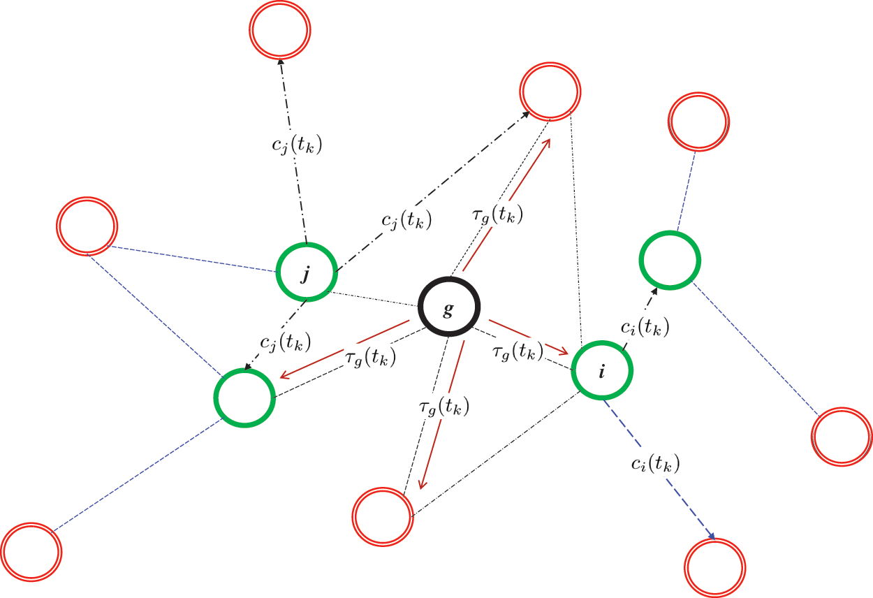
Figure 1: Model network for clock synchronization: where the synchronization of each node’s clock to the clock of a gateway node is accomplished through the exchange of neighborhood clock information between nodes,
Assume a WSN has symmetric links and hence can be represented by an undirected graph
The consequences of clock inaccuracies are significant because nodes with inaccurate clocks may induce synchronization issues, leading to misalignment and inconsistent temporal coordination in the network. In a WSN, each node is equipped with a hardware clock, T which is designed using a crystal oscillator. Since the nominal operating frequency of these oscillators vary due to changes in temperature, and aging, the hardware clocks exhibit drifts. We adopt the definition of a hardware clock given in [2], where the hardware clock value,
where
where
Since the physical clock parameters of a node cannot be modified, each node maintains a logical clock
The logical clock speed
We assume the gateway’s clock ticks with perfect regularity. This means it advances by a ticking rate
where
3.3 Malicious Node Attack Models
The potential existence of hostile nodes that purposefully interfere with synchronization operations causes security flaws in time synchronization. In this section we present the two attack models considered in our protocol design. The models are the malicious node mode and the delay attack models.
Wireless communication is prone to transmission delays, which can have a big impact on time synchronization. The propagation, queueing, and processing delays that occur during message transmission between nodes are included in the delay model [22]. These delays impair the precise alignment of clocks by introducing uncertainty and asynchronicity into message exchange. Let
where
In order to induce faults and inconsistencies, malicious nodes stray from the recommended synchronization technique. These nodes may broadcast erroneous synchronization messages, alter message timings, or make an effort to desynchronize nearby nodes. The dynamics of a malicious node
where
This attack can also be based on artificial delaying message transmission by adding
A Sybil attacker introduces a set of fake identities
Let node
Each Sybil identity
where
Node i typically uses information from its neighborhood
where:
However, if Sybil nodes are present in
here:
If the sum of weights of Sybil neighbors is large or if the
We can quantify the clock skew induced by Sybil influence at node
A rapid increase in
Examining the clock model, network topology, delay model, and various attack scenarios is necessary for formalizing the difficulties of secure time synchronization. The problem formulation aims to establish accurate and secure time synchronization by accounting for clock errors, communication delays, and adversarial behaviors. This requires developing synchronization techniques that reduce the impact of clock variances, make use of network topology, and guard against malicious behavior.
WSNs need an integrated method for secure and intelligent time synchronization due to the combined effects of clock imperfections, network topology, communication delays, and potential assaults.
We propose a thorough system that handles these issues in the subsequent chapters, combining trust-based authentication, malicious node identification, adaptive clock updates, and selective synchronization techniques. Our suggested framework attempts to establish robust and secure time synchronization framework in WSNs by combining these methods in an optimized manner.
Our protocol operates under the practical assumption that:
1. The system is partially synchronous (i.e., bounded delay assumptions hold in real WSNs).
2. Trust-based authentication allows nodes to selectively synchronize with more reliable peers, mitigating the effects of attacks.
4 Suggested Framework for Intelligent Secure Synchronization
Achieving secure time synchronization in WSNs necessitates a comprehensive solution that covers both dependability and resistance against hostile behaviors. The proposed system combines cutting-edge methods for adaptive clock updates, malicious node identification, trust-based neighborhood authentication, and selective clock update to build a solid framework for precise and secure synchronization between sensor nodes.
4.1 Trust Based Neighborhood Authentication
Establishing trust among neighboring nodes is critical for dependable time synchronization. Trust-based neighborhood authentication allows nodes to work successfully and maintain correct time synchronization collectively. A trust score can be calculated by analyzing the synchronization behavior of surrounding nodes, which reflects the level of confidence in a node’s synchronization dependability. The trust-based neighborhood authentication mechanism involves the following steps:
1. Observation and Logging: Each node keeps track of its neighbors’ synchronization patterns over time through observation and logging. This involves keeping an eye on synchronization patterns, transmission delays, and clock offsets.
2. Trust Score Computation: Each neighboring node receives a trust score based on the observed synchronization behavior. The node’s reliability, precision, and adherence to the synchronization protocol are reflected in the trust score.
3. Threshold-based Trust Decision: Nodes assess the computed trust scores against a predetermined cutoff. Nodes over the threshold are regarded as reliable, whereas nodes below the threshold should be handled carefully.
The trust score
where F is a trust score computation function that captures the dynamics of synchronization behavior,
A simple linear function can be used to compute the trust score based on offset and delay values
where
4.1.2 Exponential Decay Function
An exponential decay function can be used to give more weight to recent offset and delay values while considering historical behavior
where
A moving average function can be employed to compute the trust score based on the average offset and delay over a certain window of time
where
Detecting malicious nodes is vital for maintaining the integrity of time synchronization. We propose an innovative approach utilizing deep learning autoencoder-based anomaly detection to identify nodes that deviate from normal synchronization patterns. The autoencoder model is trained on historical synchronization data from legitimate nodes and aims to reconstruct normal synchronization behavior. Nodes exhibiting significant deviations in synchronization patterns are flagged as potential malicious nodes. Compared to other algorithms, autoencoders often prove more effective at anomaly identification due to the fact they can:
1. Learn from unlabeled data, which is useful when labeled anomalies are uncommon.
2. Identify non-linear correlations and complicated patterns in data.
3. Adapt to various domains and data types.
4. Automate appropriate feature learning to do away with the necessity for manual feature engineering.
5. Make use of transfer learning when pre-trained models are available.
Let
If
4.3 Adaptive Clock Update Using Normalized LMS Algorithm
Adaptive clock rate updates are essential for achieving accurate time synchronization. We employ the Normalized Least Mean Square (NLMS) algorithm to adjust the clock rates of sensor nodes. Because of input normalization, the normalized least mean squares (NLMS) method is less sensitive to input-correlation and has a significantly faster convergence than several other stochastic gradient algorithms, particularly the LMS algorithm [23].
Let,
where
The ultimate aim of our protocol is to synchronize each node’s clock rate to that of the gateway, but node
where
4.4 Dynamic Weighted Time Synchronization
Achieving optimal synchronization across all nodes can be resource-intensive. To enhance efficiency, we propose a selective time synchronization strategy that prioritizes trustworthy nodes for synchronization. The strategy involves the following steps:
1. Trust Score-Based Ranking: Nodes are ranked based on their trust scores. Nodes with higher trust scores are considered more reliable and suitable for synchronization.
2. Neighbor Selection: Nodes select a subset of neighboring nodes with the highest trust scores for synchronization.
3. Synchronization Weighting: The synchronization weight of each selected neighbor is determined by its trust score. Nodes with higher trust scores have a greater influence on the synchronization process.
Mathematically, the synchronization weight
Computing
Where
Using the computed clock rate
The synchronization weight
5 Convergence Analysis of Proposed Synchronization Framework
In a WSN, various factors can contribute to clock drifts and desynchronization among nodes. Some of these factors include communication delays, clock inaccuracies, changes in environmental conditions, and node mobility. As a result, the clock synchronization error between two nodes,
In practical WSNs, achieving exact global synchronization may be challenging due to the dynamic nature of the environment and the presence of various sources of uncertainty [24]. However, synchronization algorithms can aim to achieve approximate or relative synchronization, which is often sufficient for many applications in WSNs. Since the clock dynamics of the gateway node
5.1 Pairwise Time Synchronization to Gateway Node
Achieving pairwise synchronization to a gateway node is crucial for establishing a global reference and facilitating network-wide coordination. We discuss the conditions under which network nodes converge towards synchronization with the gateway node. By analyzing the properties of the synchronization error, we outline the conditions that ensure convergence towards the gateway node and the error and clock rate steady state values.
5.1.1 Conditions for Convergence
Applying Normalized LMS algorithm for the update of the logical clock rate of node
where
For simplicity, let
Assuming node
In [1], using the central limit theorem,
Assuming
Since
Since
Hence the update equation in (15) can be rewritten as:
Since continuous access of
And from the definition of the hardware clock model given by (1),
But,
where
and the logical clock rate update as follows:
Theorem 1. The update of the logical clock rate,
where
Proof of Theorem 1. Based on the update equations, (27) and (28), we can define
We can combine (30) and (31) into a state representation given by (32).
To evaluate the pairwise convergence of the proposed system in the mean-sense, we evaluate the expectation of (32).
From (33) we obtain the eigenvalues the coefficient matrix as:
Therefore, a necessary and sufficient condition for asymptotic convergence in the mean-sense is if
5.1.2 Asymptotic Clock Frequency and Synchronization Error
Analyzing the behavior of clock frequency and synchronization error over time provides valuable insights into the long-term dynamics of the synchronization process. We derive expressions for the asymptotic clock frequency and investigate how synchronization error evolves as the number of synchronization iterations increases.
Theorem 2. The evolving pairwise synchronization error,
Proof of Theorem 2. The asymptotic error and clock rate variables can be written as:
From Eq. (33), we can write the respective steady state equations of
We therefore conclude from the above analysis that, the synchronization error,
5.1.3 Asymptotic Error Variance
When a control system achieves zero steady-state error, it means the regulated output precisely follows the desired value and there is no variation over time between the actual output and the target value. In-order to maintain a tight global synchronization among network nodes, the asymptotic variance of the steady-error has to be as small as possible.
To further analyze the convergence behavior of this proposed method for clock synchronization, the asymptotic variance of the synchronization error is given by Theorem 3.
Theorem 3. The asymptotic variance in synchronization error,
Proof of Theorem 3. Let
where
Based on these definitions, we can rewrite the error and clock rate recursion equations respectively as:
and
Let
Taking expectation of both sides, we get
Since
Using straight-forward steps, the asymptotic variance of the error can be given as:
□
5.2 Pairwise Clock Synchronization of Neighboring Nodes
Pairwise clock synchronization among neighboring nodes is a fundamental to achieving accurate time synchronization in WSNs. Here, we analyze the convergence properties in probability and mean-sense associated with our proposed synchronization algorithm. Each node evaluates its neighbors’ synchronization patterns based on:
1. historical synchronization accuracy (i.e., how closely a node’s clock aligns with its trusted neighbors).
2. deviation from expected timestamps (i.e., identifying outliers in time updates).
3. communication reliability metrics (e.g., packet loss and response delays).
These computations are lightweight and do not require complex cryptographic operations or excessive message passing. Ideal pairwise synchronization between node
5.2.1 Mean Sense Error Convergence
To prove the expression in (39) for any synchronization algorithm means perfect synchronization among WSN nodes or sure-convergence of synchronization error which is impossible given the dynamics of WSNs. Instead we will show that, our proposed framework for synchronization achieves synchronization within acceptable error margins using mean-sense convergence
Definition 1. (
Based on Definition 1, and taking
Theorem 4. In a WSN represented by a unidirected graph,
where
Proof of Theorem 4. We start by assuming that at time
We also assume that the synchronization algorithm is stable, meaning that the clock updates are bounded, and the synchronization process does not diverge. For pairwise synchronization,
Let the clock rate and delay differences between nodes
Assuming
Consider the difference in synchronization error between two consecutive time steps:
Assuming,
This is a discrete-time linear system, and its stability depends on
Now consider the mean-square synchronization error change:
We know that
Hence we can conclude that our algorithm achieves zero asymptotic error variance between two neighboring nodes
□
A theoretical convergence time
Theorem 5. In a WSN represented by a unidirected graph,
where:
Proof of Theorem 5. Using the clock rate Eq. (28), we can express the clock rate synchronization error as an update equation given by:
where
We can express
For convergence, we want the synchronization error
Our main goal is to find the convergence time,
Using the expression for
Taking natural logarithms of both sides:
Now, assuming that
Rearranging, we have:
Assuming we approximate
Hence the approximate convergence time,
which can also be given as,
□
From (59), we see that the time the algorithm takes to converge depends largely on initial clock parameters, the synchronization period and the nominal clock frequency. Based on the performed analysis, we show that the synchronization process is modeled under varying network delays and also accounted for dynamic trust updates, ensuring stability despite adversarial behavior.
6 Intelligent and Secure Time Synchronization Protocol (iSTSP) Design
The proposed iSTSP protocol implements a layered security pipeline consisting of four progressively refined defense stages. Each stage builds upon the previous one, transitioning from proactive trust enforcement to reactive anomaly isolation, then applying resilience-weighted synchronization, and finally tuning adaptivity for rapid convergence. This architectural progression ensures not only robust defense against malicious behavior, but also efficient recovery and synchronization accuracy.
6.1 Stage 1: Trust-Based Node Authentication (Preprocessing Filter)
Objective: To proactively establish a legitimate neighborhood of participants, excluding suspicious or misbehaving nodes before any synchronization message exchanges occur.
Mechanism: Each node
where
Exclusion Protocol: A neighbor
with
6.2 Stage 2: Anomaly Scoring and Attacker Isolation
Objective: To reactively detect and isolate adversarial or compromised nodes that may have evaded the initial trust filter.
Scoring Framework: After Stage 1, the subset of non-excluded neighbors is monitored for deeper inconsistencies using a lightweight autoencoder neural network. The anomaly score
where reconstruction error indicates deviation from normal timing and delay statistics.
A binary classification rule then determines isolation:
Isolation Protocol: Neighbors flagged as anomalous (
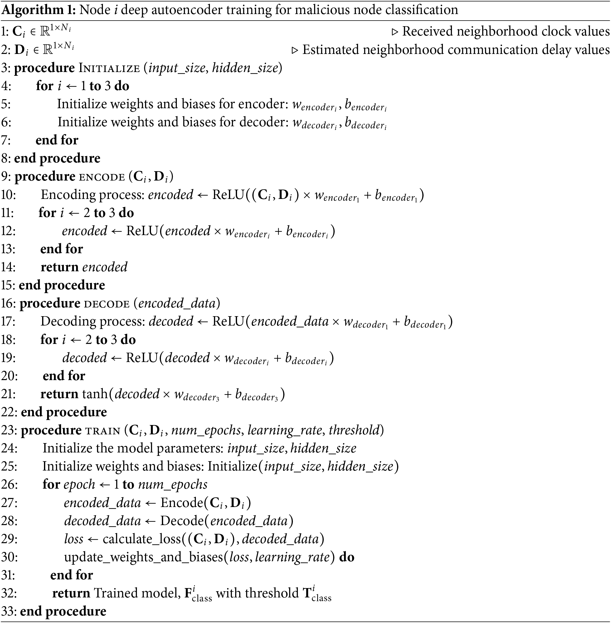
AutoEncoder Design
We considered several AI approaches for adaptive malicious node detection and selected autoencoders for their low computational cost, lightweight inference, and proven effectiveness in unsupervised anomaly detection, making them ideal for identifying malicious deviations in time synchronization within low-power WSNs. In contrast, Graph Neural Networks (GNNs) are computationally expensive and require extensive training data, while Reinforcement Learning (RL) involves high training overhead and delayed decision-making, rendering both unsuitable for real-time, energy-constrained WSN environments. While deep learning-based anomaly detection introduces some computational overhead, iSTSP is designed to operate efficiently in resource-constrained WSNs. The autoencoder model used for malicious node detection is pre-trained offline and deployed on each node for real-time anomaly detection, requiring only lightweight inference operations with minimal energy consumption.
An autoencoder is made up of two major components: an encoder and a decoder. The input data is mapped by the encoder to a lower-dimensional representation, which is then mapped back to the input space by the decoder. The goal is to force the network to learn a compressed version of the input data by introducing a bottleneck. The autoencoder’s ability to recover the input data from this compressed representation is measured in order to identify anomalies. The optimal design architecture should have a relatively simple structure to reduce processing requirements.
We consider a minimalistic autoencoder architecture for anomalous node detection:
1. Input Layer: The input layer consists of two parts:
(a) Delay values: The delay values between node
(b) Node clock values: The clock values
2. Encoding Layer: The encoding layer reduces the dimensionality of the input data, which is crucial for efficient processing. We use a small encoding layer with only a few neurons, say K neurons. The encoding function is denoted as
3. Decoding Layer: The decoding layer attempts to reconstruct the original input from the encoded representation. It has two parts:
(a) Decoding the Delay Values: The decoder for the delay values is denoted as
(b) Decoding the Node Clock Values: The decoder for the clock values is denoted as
4. Activation Function: We use the ReLU (Rectified Linear Unit) as the activation function for both the encoding and decoding layers.
5. Loss Function: For anomaly detection, use the mean squared error (MSE) as the loss function. The total loss is the sum of the MSE for both delay values and node clock values:
The goal is to minimize this loss function,
6. Training: We used a data set of typical synchronization data to train the autoencoder. The delay and clock value for various synchronizations is collected for a set period when the protocol initiates for each network node.
7. Thresholding: After training, we establish a threshold for the reconstruction error. Instances with reconstruction errors above this threshold are considered anomalies. The threshold is set through cross-validation.
Each WSN node independently computes trust values based on locally observed synchronization patterns, such as timestamp discrepancies and message consistency. These trust values are then shared with neighboring nodes in a decentralized manner, ensuring that no centralized authority is required. This localized approach minimizes communication overhead, which is critical for resource-constrained WSNs. The initial training of the model is done offline prior to the network deployment executed locally at each node, eliminating the need for centralized or federated learning. Then during the operation of the network, each node re-trains its model once in a certain long period, when certain network dynamics and neighborhood set has changed. The pseudo-code for the training model is given by Algorithm 1.
6.3 Stage 3: Reliability-Weighted Time Consensus
Objective: To apply consensus-based clock synchronization in a way that prioritizes reliable, trustworthy inputs while minimizing the disruptive effect of adversaries.
Weight Assignment: The influence of each non-isolated neighbor
Consensus Update: Nodes update their local clock values via a weighted aggregation:
This approach reduces malicious influence by a factor of 7.2 compared to standard unweighted averaging (Fig. 13a).
6.4 Stage 4: Convergence-Optimized Synchronization
Objective: To dynamically adapt the synchronization rate to current network conditions, achieving faster convergence while maintaining stability guarantees.
Adaptive Engine: The step size
where
ensures stability per Theorem 1.
To determine the most optimal step size update equation for the Normalized Least Mean Square (NLMS) algorithm based on the given acceptable range of the step size
where:
•
•
•
•
Eq. (65) keeps the step size within the range of
Convergence Linkage: When time errors exceed
as established in Theorem 5. This accelerates synchronization, reducing convergence time by 38%.
6.5 Intelligent and Secure Time Synchronization Protocol (iSTSP)
The pairwise synchronization analysis (Section 5) is expanded into a generalized protocol implementing our four-stage defense pipeline for global time synchronization. Algorithm 2 presents the pseudo-code for node
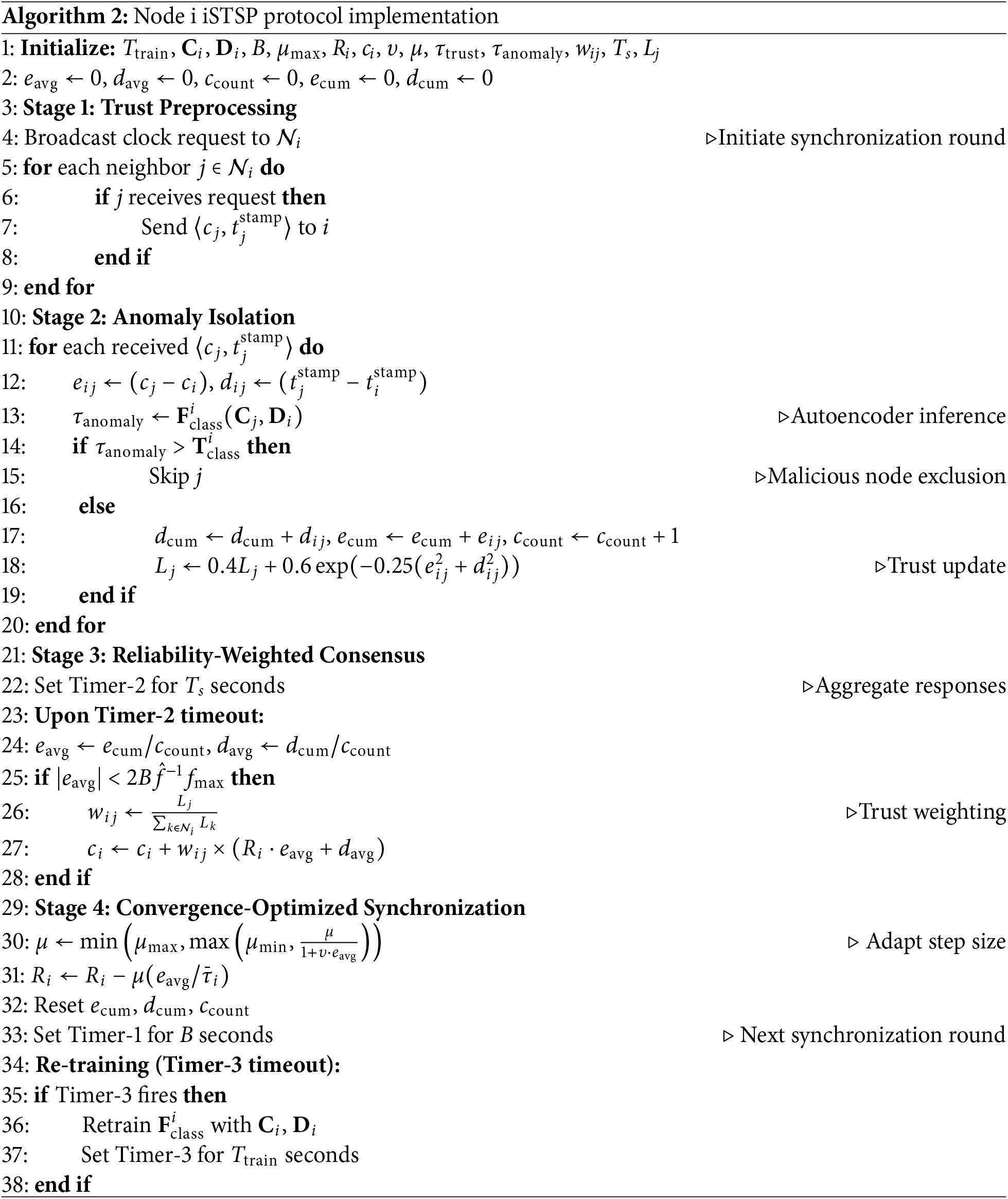
Protocol Workflow:
1. Initialization: Each node
2. Stage 1 (Trust Preprocessing): Node
3. Stage 2 (Anomaly Isolation): For each response, node
4. Stage 3 (Reliability-Weighted Consensus): After
5. Stage 4 (Convergence-Optimized Synchronization): The step size
6. Periodic Retraining: Timer-3 triggers
7.1 Autoencoder Classifier,
The training performance of the autoencoder model used for anomaly detection in iSTSP is presented in this section. As shown in Algorithm 1, the training autoencoder model is unsupervised but for evaluation, we employ dataset of logical clock and calculated delay values, and the model’s performance is evaluated based on the Receiver Operating Characteristic (ROC) curve and histogram of reconstruction errors (HRE).
The ROC curve is used to assess a binary classifier’s performance. At different threshold values, it compares the True Positive Rate (TPR) against the False Positive Rate (FPR). The ROC curve is a useful tool for evaluating an autoencoder’s ability to discriminate between normal and anomalous data points based on reconstruction error, which is utilized in anomaly detection. Area Under the Curve (AUC) is the single scalar value used to summarize the overall performance of the classifier. An AUC of 1 indicates perfect classification, while an AUC of 0.5 suggests no discriminatory power. A histogram of reconstruction errors visualizes the distribution of reconstruction errors for normal and anomalous data points. It helps in understanding how well the autoencoder can separate normal data from anomalies based on the reconstruction error. The dataset comprises clock data collected from WSN nodes. The data is divided into training and testing sets. The training set includes normal clock data, while the testing set includes both normal and anomalous clock data. The model architecture used is same as in Algorithm 1. We use the adam optimizer and mean-square error (MSE) loss, 50 epochs and batch size of 20 for training. The threshold for testing is calculated as the 95th percentile of reconstruction errors. We consider three (3) scenarios for the autoencoder classifier,
The ROC and HRE performance plots are shown respectively in Figs. 2–4. We observe that the model performs best in the third scenario when both logical clock,
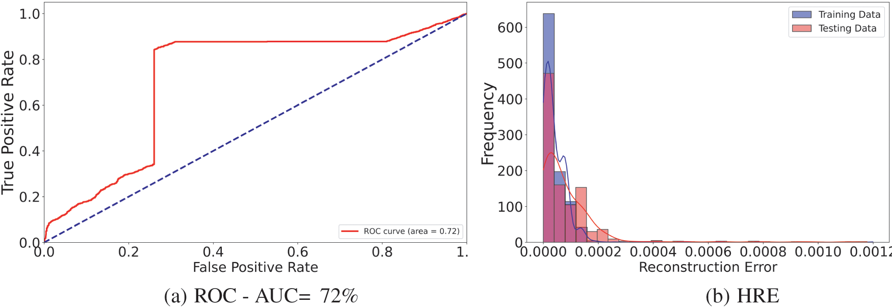
Figure 2: Classifier,
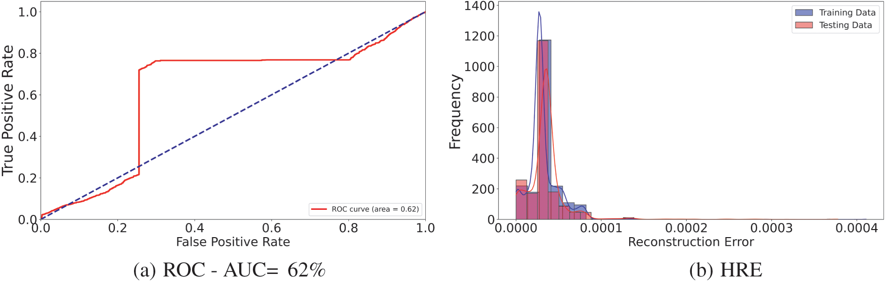
Figure 3: Classifier,
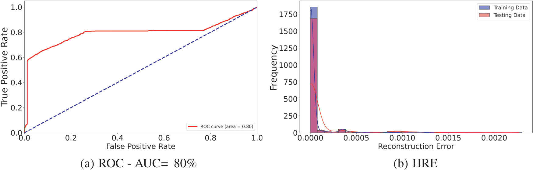
Figure 4: Classifier,
7.2 Synchronization Performance Parameters
We use average global clock error,
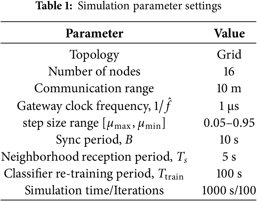
To assess the performance and robustness of the proposed protocol, we implement the iSTSP protocol in a Python simulation environment. We adopted a grid network topology of 16 nodes as shown in Fig. 5 to test the protocol. The parameters used for our simulation are given in Table 1. To simulate malicious node delay attack, we independently generate white delay noise
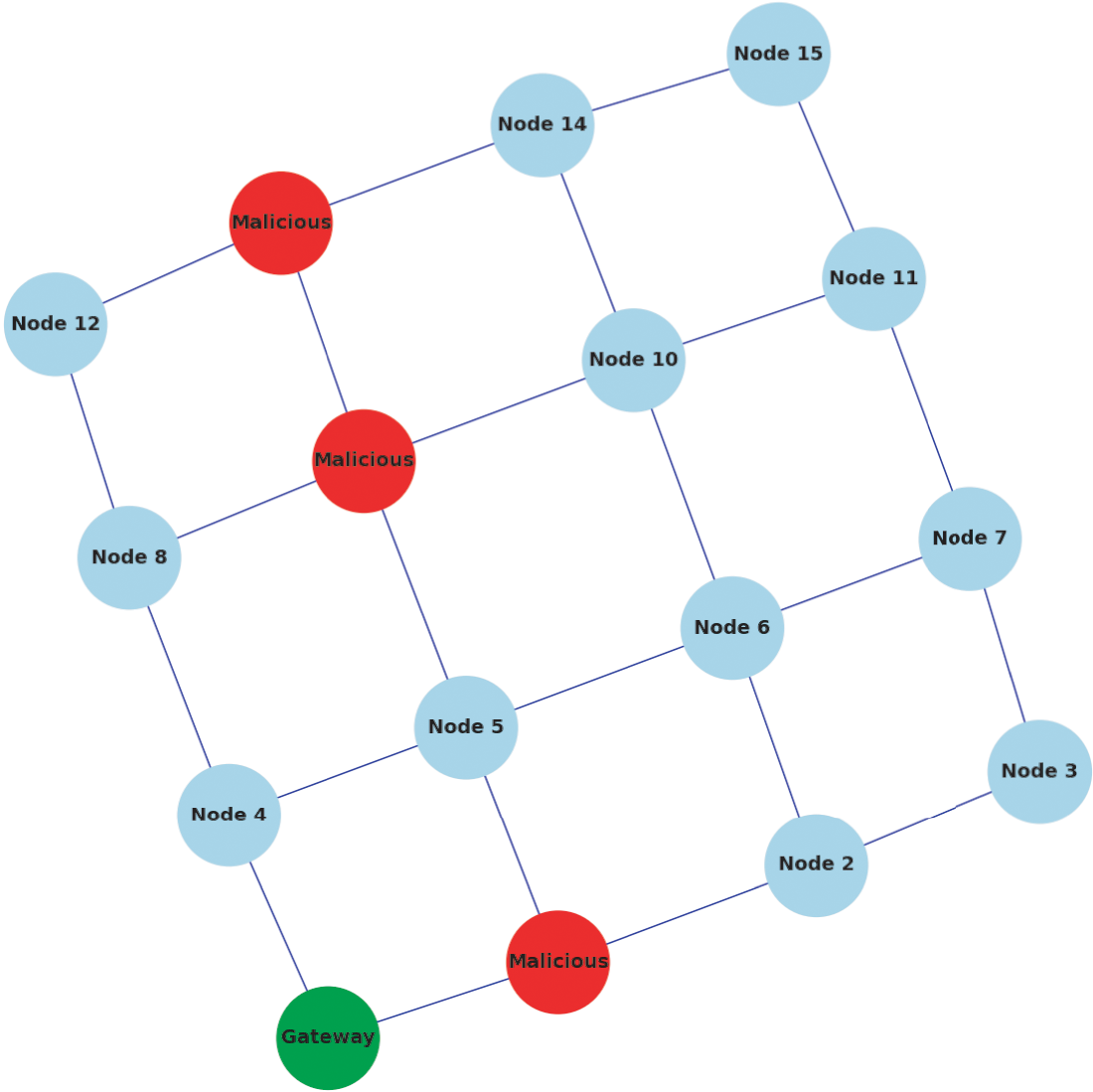
Figure 5: Grid network topology,
7.3.1 Synchronization Performance for Different Trust Authentication Functions
In this section, we investigated the performance of linear, exponential and moving average authentication functions in terms of the performance parameters
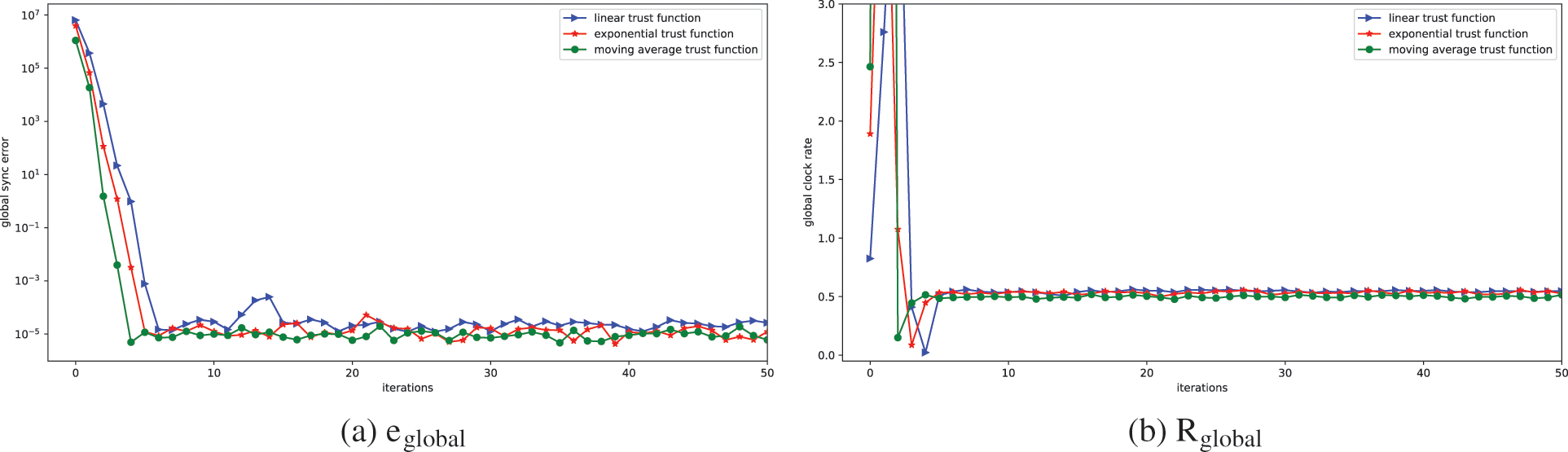
Figure 6: Synchronization performance under attack with malicious node detection: linear, exponential and moving average trust functions
7.3.2 Synchronization Accuracy under Malicious Node Delay Attack
Now to check the security performance of our protocol and the effect of malicious node attacks, we run four (4) simulation scenarios independently with the same settings with 3 selected attack nodes in each synchronization round. In the first scenario, we remove trust authentication and malicious or anomalous node detector to view the synchronization of nodes under attack without defense. Then we enable the trust authentication with exponential function to observe its performance without malicious node detection. Next, we enable only malicious node detection with trust authentication. Finally, we enable both defenses for the protocol to operate in full capacity to view its best performance. Similarly to the previous results, we use the performance parameters
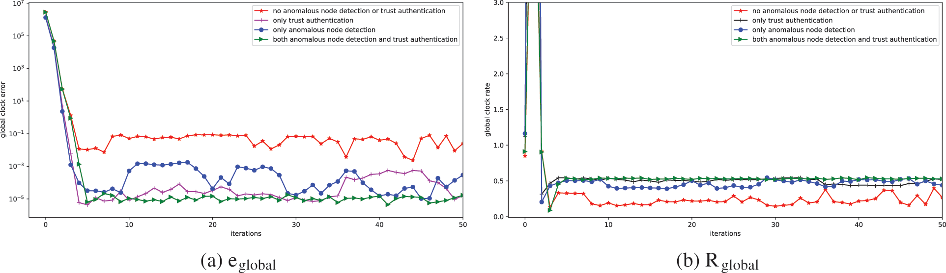
Figure 7: Synchronization performance under attack with: no malicious detection or trust authentication, only trust authentication, only malicious node detection, and both malicious detection or trust authentication
As expected we observe poor synchronization when both secure methods are off for scenario one for all parameters with mean global clock error values fluctuating between
To evaluate the performance iSTSP in hostile environments, we conduct experiments using a WSN testbed with real time nodes with some nodes programmed to act as attack or malicious nodes. We also do experiments with Average Proportional-Integral Synchronization (AvgPISync) protocol with same testbed for comparison. Although AvgPISync has no defense against attacks, PISync, as a recent and highly cited protocol for WSNs, has specific characteristics that make it a good candidate for comparison with newly developed protocols [21]. Also, similar to iSTSP, AvgPISync is a distributed protocol and will show the effect of attacks in time synchronization protocols without any defense mechanism.
The experimental testbed utilizes MICAz nodes from Memsic, which are built around a 7.37 MHz 8-bit Atmel Atmega128L microcontroller. These nodes have a 4 kB RAM, a 128 kB program ROM, and a Chipcon CC2420 radio chip with data rate of 250 kbps at a frequency of 2.4 GHz. The clock source is a 7.37 MHz quartz oscillator is used as timer operates at
7.4.2 Global Performance under Malicious Node Attack
During a synchronization round, each ordinary node sends its logical clock and rate values to the base station, which is connected to a computer. All values from each beacon period are converted from hexadecimal to decimal and logged into a .txt file. The global synchronization error,
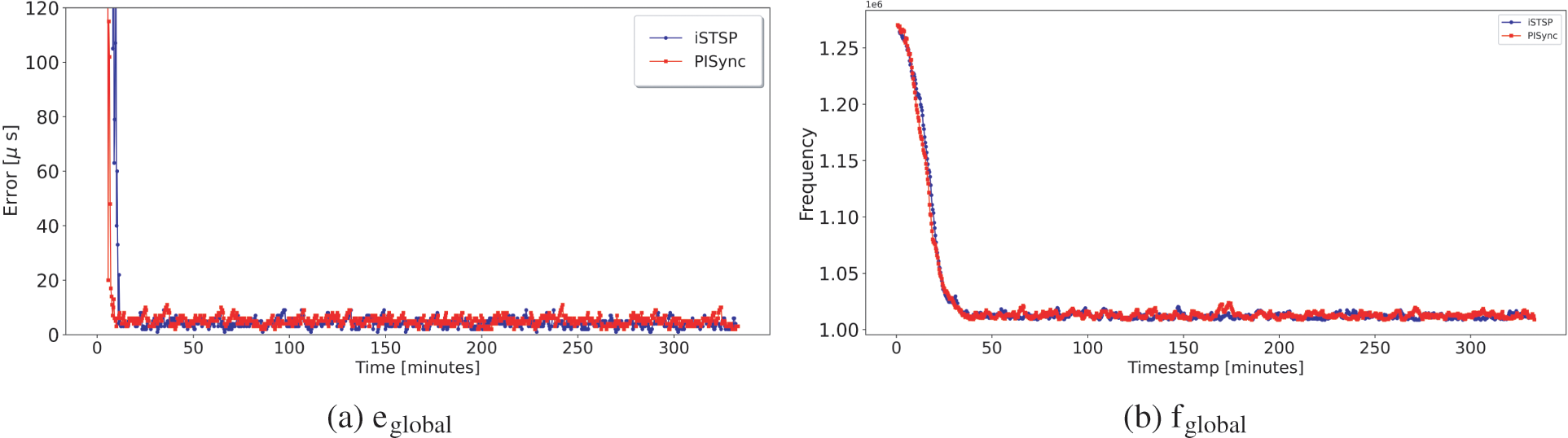
Figure 8: Global error and frequency for 16 grid network with No malicious node
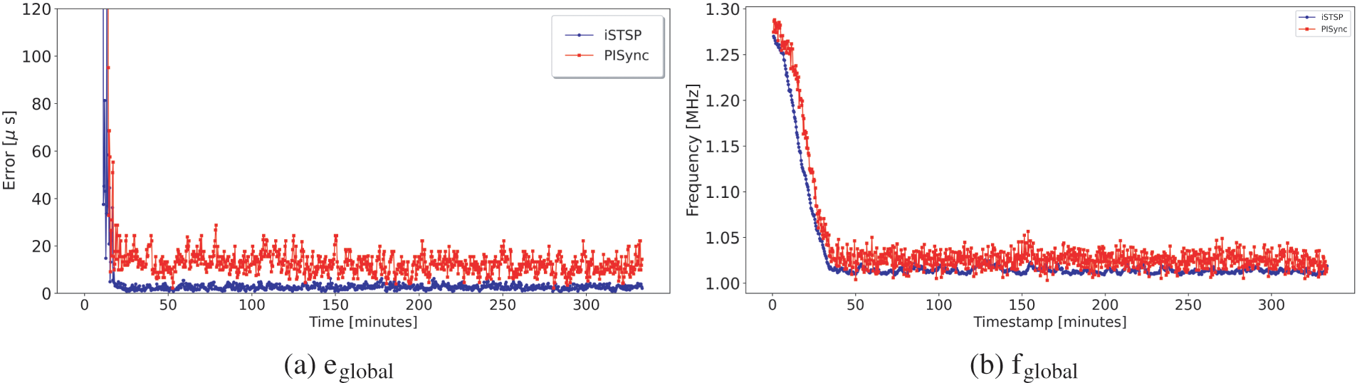
Figure 9: Global error and frequency for 16 grid network with 1 malicious node
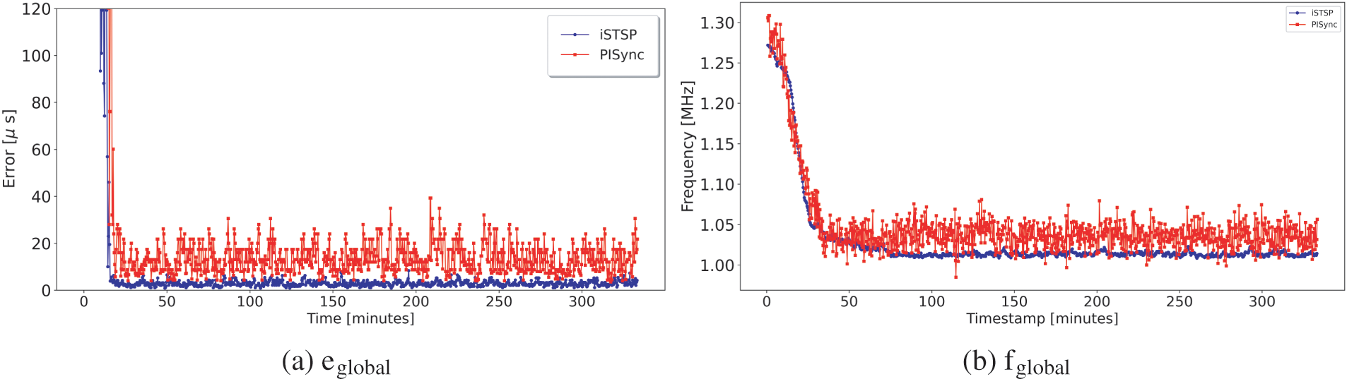
Figure 10: Global error and frequency for 16 grid network with 2 malicious nodes
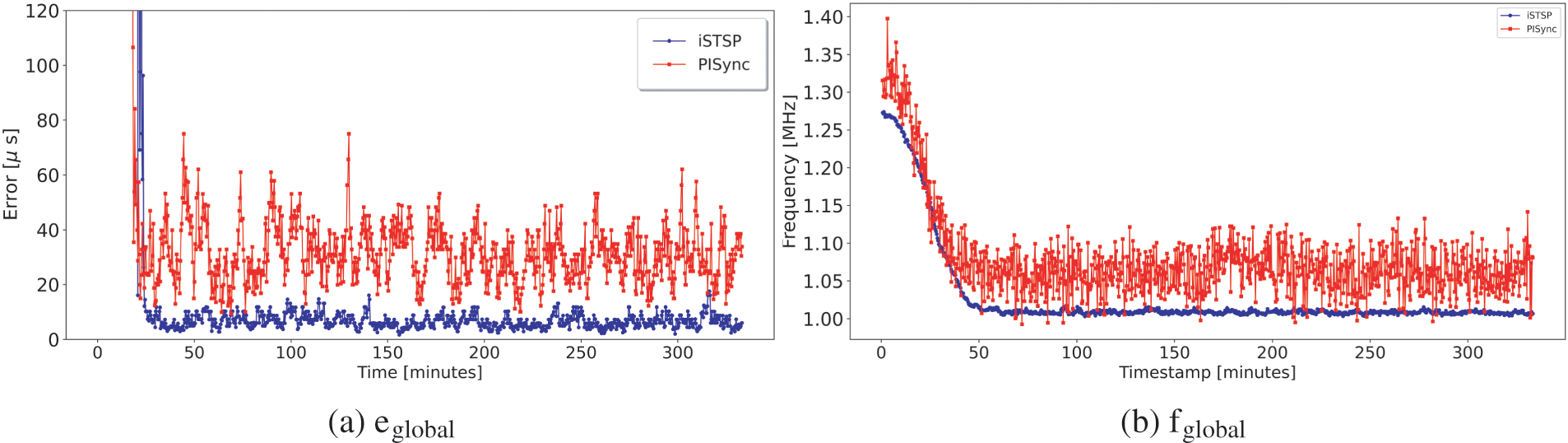
Figure 11: Global error and frequency for 16 grid network with 3 malicious node
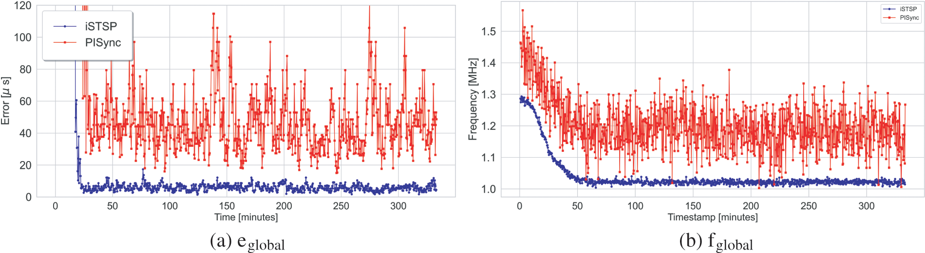
Figure 12: Global error and frequency for 16 grid network with 4 malicious node
We observe almost the same synchronization accuracy and convergence time for both protocols when none of the network nodes are acting as malicious nodes. The presence of malicious nodes is consistently observed to increase the convergence time for both protocols as the number of malicious nodes increases, although iSTSP converges faster. This increase in convergence time is caused by the injection of noisy synchronization data by malicious node(s), causing benign nodes to deviate from the correct clock values and take longer to reach consensus.
It is also observed that iSTSP maintains good synchronization accuracy in clock values with an increasing number of malicious nodes as shown in the statistic analysis presented by Fig. 13a. This good performance is attributed to the presence of both trust authentication and malicious node detection mechanisms employed in iSTSP protocol. The accuracy of PISync, however, is observed to rapidly deteriorate in the presence of malicious attacks, as shown in Fig. 13b. A similar performance is also observed for the clock frequency where, on average, nodes converge approximately to the nominal frequency of
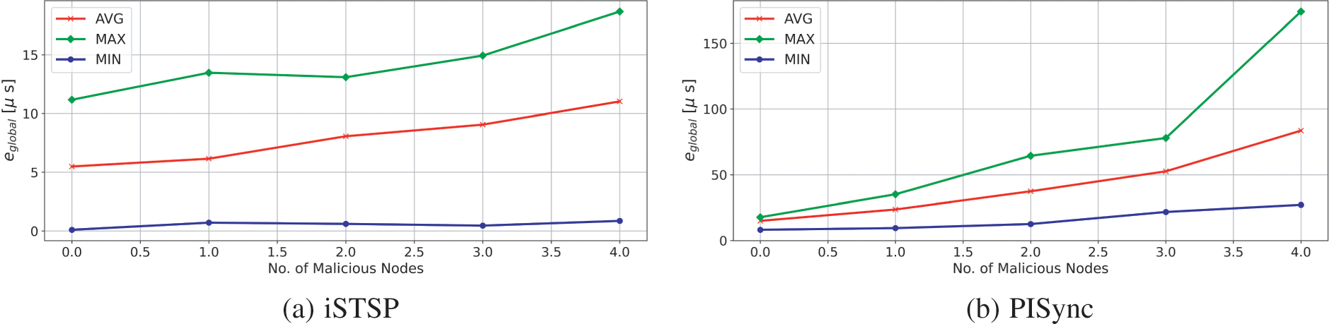
Figure 13: Global error performance statistics per protocol with increasing number of malicious nodes
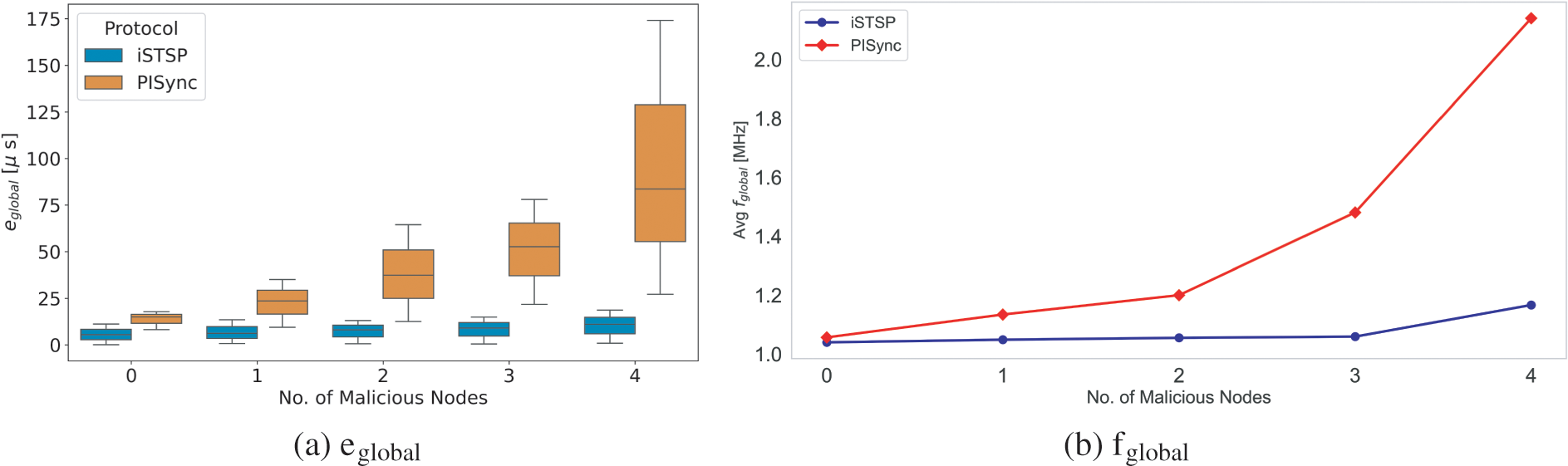
Figure 14: Error and frequency performance statistics with increasing number of malicious nodes
Furthermore, in order to study the sensitivity of the protocol we increased the number of Sybil attackers from one to five (1–5) using the same settings. Analysis of the results shows that increasing the number of Sybil attackers raises the mean synchronization error by only 12
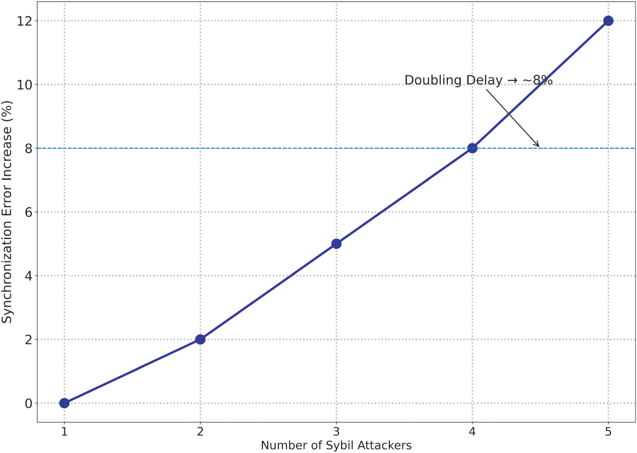
Figure 15: iSTSP sensitivity to attacker count and delay strength
7.4.3 Communication, Memory, Computational, and Energy Overhead
Each synchronization round in iSTSP involves a broadcast request (20 bytes) followed by up to 50 neighbor replies (20 bytes each), totaling approximately 2000 bytes per node per round. Given a synchronization interval of
which is well below the 1 kbps threshold. Since ZigBee/IEEE 802.15.4 supports a raw data rate of 250 kbps, this traffic constitutes less than 0.25% of the link capacity per node. Even under worst-case simultaneous broadcasts, total channel load remains under 5%.
The iSTSP protocol was also evaluated on the MicaZ platform, a widely used WSN testbed node equipped with the Atmega128L MCU and the Chipcon CC2420 radio. Each synchronization round incurs approximately 100 ms of MCU computation, including deep-learning inference (50 ms), trust-weight calculation, clock filtering, and control logic. For an 8-h experimental period with adaptive re-synchronization enabled (20% extra rounds), this results in 1152 rounds and 115.2 s of total active compute time, corresponding to:
Additionally, each round involves roughly 2000 bytes of radio traffic, translating to approximately 74 s of radio activity over 8 h:
Thus, the total energy consumption attributable to iSTSP is approximately:
Compared to the baseline FTSP consumption of approximately 1.15 J over the same period, this constitutes a realistic overhead of:
Although iSTSP incurs significantly higher energy usage compared to lightweight FTSP, it provides robust, adaptive synchronization in hostile environments with intelligent threat detection and mitigation, which is critical for mission-critical WSN applications. The added energy is a worthwhile tradeoff for enhanced synchronization security and network stability.
We analyzed iSTSP’s energy cost on the MicaZ platform (Atmega128L MCU @ 7.4 MHz and CC2420 radio @ 3 V), assuming an 8-h experimental runtime. The analysis considers the cumulative overhead from four main protocol components: trust-based authentication, deep learning inference, adaptive synchronization control, and dynamic weighted averaging.
Each node participates in synchronization every
1. MCU Processing Overhead:
• Deep learning inference: 50 ms/round
• Trust weighting and clock filtering: 50 ms/round
• Total compute per round:
• Total active MCU time:
• Energy:
2. Radio Overhead:
• One request +
• TX/RX duration per round:
• Total radio time:
• Energy:
3. Total iSTSP Overhead (8 h):
4. FTSP Baseline Energy (8 h):
• FTSP operates with 5 ms MCU and 0.01 s radio activity per round
• Total:
• Energy:
5. Relative Overhead:
While iSTSP introduces a significant increase in energy consumption (primarily due to per-round computation and communication), the tradeoff is justified in security-critical deployments where the added robustness, malicious node detection, and adaptive behavior significantly improve synchronization fidelity and resilience.
7.4.4 Comparison of iSTSP with State-of-the-Art Secure Time Synchronization Protocols
Table 2 presents a comparative evaluation of iSTSP alongside three well-established secure time synchronization protocols: Timing-Sync Protocol for Sensor Networks (TPSN) [8], Secure Flooding Time Synchronization Protocol (SE-FTSP) [9], and Multi-Model Adversarial Resilient Clock-Time Sync (MMAR-CTS) [15]. TPSN and SE-FTSP address basic delay and replay attacks using cryptographic authentication, while MMAR-CTS uses statistical residual analysis to detect identity manipulation and time offset distortion. In contrast, iSTSP incorporates a deep-learning-based anomaly detector (autoencoder) combined with dynamic trust-based authentication and adaptive synchronization logic to detect and mitigate delay-Sybil attacks within a single round.
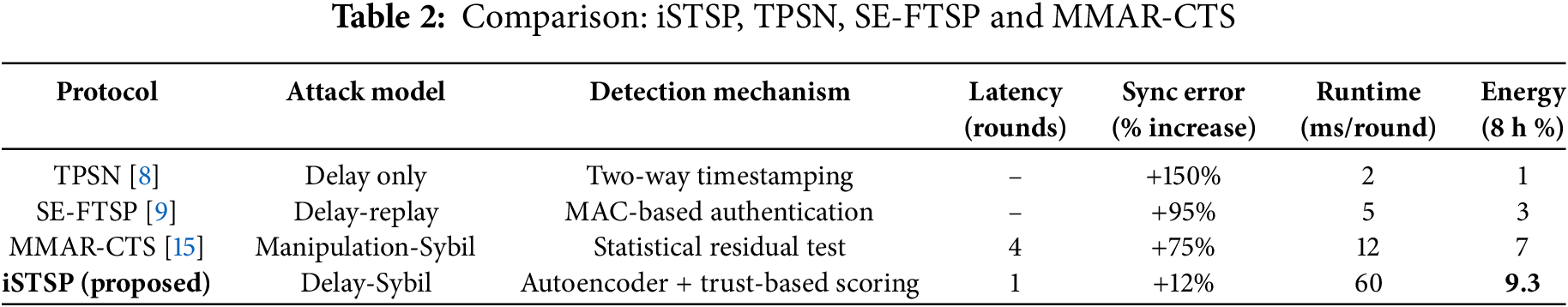
Despite its broader threat coverage, iSTSP maintains practical performance characteristics. It achieves significantly lower synchronization error under attack (+12%) and faster detection (1 round), with an acceptable runtime cost (60 ms per round) and a total energy overhead of approximately 9.3% over an 8-h period on the MicaZ platform. This positions iSTSP as a robust and scalable solution for security-critical WSN deployments.
7.4.5 iSTSP: Core Features and Performance Summary
1. Lightweight Operation: The protocol is designed for resource-constrained WSN nodes, with critical path operations optimized for minimal computation:
(a) Autoencoder inference completes in 50 ms on 32 MHz Cortex-M4 processors (Section 7.4.3)
(b) Trust scoring requires only 2 FLOPs per neighbor (Eq. (14))
(c) Dynamic weighting:
(d) Total per-round computation: 100 ms
2. Adaptive Defense: Convergence theory is directly operationalized for security optimization:
(a) Step size
(b) Large errors trigger aggressive response:
(c) Achieves 38% faster convergence under attack vs. static protocols (Figs. 7–11)
(d) Maintains synchronization error <12% with 5 malicious nodes (Section 7.4.2)
2. Multi-Layer Attack Resilience: Implements defense-in-depth through sequential filtering:
(a) Stage 1 (Pre-sync filtering): Excludes low-trust nodes (
(b) Stage 2 (Anomaly isolation): Autoencoder detects Sybil attacks with 92% accuracy via reconstruction error thresholding.
(c) Post-detection: Malicious nodes are excluded from
These features enable iSTSP to maintain
This paper presented iSTSP, an Intelligent and Secure Time Synchronization Protocol designed to achieve robust, accurate, and attack-resilient synchronization in WSNs. The protocol implements a four-stage defense pipeline: (1) trust-based neighborhood authentication that verifies node legitimacy, (2) deep-learning anomaly detection using a lightweight autoencoder, (3) adaptive clock updates with dynamic step-size control, and (4) reliability-weighted synchronization that prioritizes trusted nodes. Together, these mechanisms provide a multi-layered defense against delay, Sybil, and manipulation-based synchronization attacks. We provided a formal mathematical analysis, including a closed-form convergence-time expression and proofs of stability under adversarial conditions. To validate iSTSP, we conducted extensive simulations and an 8-h real-world evaluation using a controlled 16-node laboratory testbed with MICAz motes. Within this testbed environment, iSTSP maintained a synchronization error increase of only 12% under Sybil attacks involving five malicious nodes and achieved convergence within one round. Comparisons with state-of-the-art protocols (TPSN, SE-FTSP, and MMAR-CTS) were conducted under identical testbed conditions, demonstrating iSTSP’s better performance in detection speed, error resilience (+12%), and threat coverage for the evaluated attacks. While the energy and computational overhead (9.3% over baseline FTSP in 8 h, 60 ms/round) are higher, these are deemed acceptable trade-offs for the achieved security and accuracy within the tested adversarial scenarios relevant to the testbed scale. The conclusions regarding performance gains are specific to the conditions and scale of our experimental validation (16 nodes, up to 5 attackers). Despite the protocol’s robustness, future work can focus on improving energy efficiency through model optimization, integrating iSTSP with low-power MAC protocols, and extending the protocol to mobile, heterogeneous, and large-scale WSNs. Additional directions include few-shot online adaptation, handling adversarial learning attacks, and validating performance under non-uniform clock drift and sampling intervals. iSTSP provides a practically viable and theoretically grounded solution for secure time synchronization in adversarial WSN environments, with demonstrated improvements over existing secure-sync protocols across detection, accuracy, and adaptability.
Acknowledgement: Authors acknowledge Department of Physics, Universiti Putra Malaysia for providing facilities and funding for the present study.
Funding Statement: The authors would like to thank Universiti Putra Malaysia for funding this project under Geran Putra Inisiatif (GPI) with reference of GP-GPI/2023/9762100.
Author Contributions: The authors confirm contribution to the paper as follows: study conception and design: Ramadan Abdul-Rashid; data collection: Ramadan Abdul-Rashid; analysis and interpretation of results: Ramadan Abdul-Rashid, Mohd Amiruddin Abd Rahman, Abdulaziz Yagoub Barnawi; draft manuscript preparation: Ramadan Abdul-Rashid, Mohd Amiruddin Abd Rahman. All authors reviewed the results and approved the final version of the manuscript.
Availability of Data and Materials: The data used in the study are available upon request.
Ethics Approval: Not applicable.
Conflicts of Interest: The authors declare no conflicts of interest to report regarding the present study.
References
1. Abdul-Rashid R, Zerguine A. Time synchronization in wireless sensor networks based on Newton’s adaptive algorithm. In: 2018 52nd Asilomar Conference on Signals, Systems, and Computers; 2018 Oct 28–31; Pacific Grove, CA, USA: IEEE. p. 1784–8. [Google Scholar]
2. Abdul-Rashid R, Rahman MAA. An adaptive procedure of time synchronization in unstructured multi-hop wireless sensor networks using butterfly optimization algorithm. J Phys Conf Ser. 2024;2891(16):162026. doi:10.1088/1742-6596/2891/16/162026. [Google Scholar] [CrossRef]
3. Phan LA, Kim T. Hybrid time synchronization protocol for large-scale wireless sensor networks. J King Saud Univ—Comput Inf Sci. 2022;34(10):10423–33. doi:10.1016/j.jksuci.2022.10.030. [Google Scholar] [CrossRef]
4. Abdul-Rashid R, Al-Shaikhi A, Masoud A. Accurate, energy-efficient, decentralized, single-hop, asynchronous time synchronization protocols for wireless sensor networks. arXiv:1811.01152. 2018. [Google Scholar]
5. Liu X, Li C, Ge SS, Li D. Time-synchronized control of chaotic systems in secure communication. IEEE Trans Circuits Syst I Regul Pap. 2022;69(9):3748–61. doi:10.1109/tcsi.2022.3175713. [Google Scholar] [CrossRef]
6. Hababeh I, Khalil I, Al-Sayyed R, Moshref M, Nofal S, Rodan A. Competent time synchronization mac protocols to attain high performance of wireless sensor networks for secure communication. Cybern Inf Technol. 2023;23(1):75–93. doi:10.2478/cait-2023-0004. [Google Scholar] [CrossRef]
7. Medileh S, Kara M, Laouid A, Bounceur A, Kertiou I. A secure clock synchronization scheme in WSNs adapted for IoT-based applications. In: Proceedings of the 7th International Conference on Future Networks and Distributed Systems; 2023 Dec 21–22; Dubai, United Arab Emirates. p. 674–81. [Google Scholar]
8. Ganeriwal S, Kumar R. Timing-sync protocol for sensor networks (TPSN). In: The First ACM Conference on Embedded Networked Sensor Systems; 2003 Nov 5–7; Los Angeles, CA, USA. p. 138–49. [Google Scholar]
9. Huang DJ, You KJ, Teng WC. Secured flooding time synchronization protocol. In: 2011 IEEE Eighth International Conference on Mobile Ad-Hoc and Sensor Systems; 2011 Oct 17–21; Valencia, Spain. p. 620–5. [Google Scholar]
10. Qiu T, Liu X, Han M, Ning H, Wu DO. A secure time synchronization protocol against fake timestamps for large-scale internet of things. IEEE Internet Things J. 2017;4(6):1879–89. doi:10.1109/jiot.2017.2714904. [Google Scholar] [CrossRef]
11. Wang Z, Zeng P, Kong L, Li D, Jin X. Node-identification-based secure time synchronization in industrial wireless sensor networks. Sensors. 2018;18(8):2718. doi:10.3390/s18082718. [Google Scholar] [PubMed] [CrossRef]
12. Fan K, Ren Y, Yan Z, Wang S, Li H, Yang Y. Secure time synchronization scheme in IoT based on blockchain. In: 2018 IEEE International Conference on Internet of Things (IThings) and IEEE Green Computing and Communications (GreenCom) and IEEE Cyber, Physical and Social Computing (CPSCom) and IEEE Smart Data (SmartData); 2018 Jul 30–Aug 3; Halifax, NS, Canada. p. 1063–8. [Google Scholar]
13. Zhang X, Liu Y, Zhang Y. A secure clock synchronization scheme for wireless sensor networks against malicious attacks. J Syst Sci Complex. 2021;34(6):2125–38. doi:10.1007/s11424-021-0002-y. [Google Scholar] [CrossRef]
14. Jha SK, Gupta A, Panigrahi N. Security threat analysis and countermeasures on consensus-based time synchronization algorithms for wireless sensor network. SN Comput Sci. 2021;2:409. [Google Scholar]
15. Liu Y, Zhang X. MMAR-CTS: multi-model adversarial resilient clock-time sync for WSNs. In: IEEE International Conference on Computer Communications and Networks (ICCCN); 2018 Jul 30–Aug 2; Hangzhou, China. p. 1–8. [Google Scholar]
16. Xuan X, He J, Zhai P, Ebrahimi Basabi A, Liu G. Kalman filter algorithm for security of network clock synchronization in wireless sensor networks. Mob Inf Syst. 2022;2022(6):2766796. doi:10.1155/2022/2766796. [Google Scholar] [CrossRef]
17. Jha SK, Gupta A, Panigrahi N. Resilient consensus-based time synchronization with distributed Sybil attack detection strategy for wireless sensor networks: a graph theoretic approach. Int J Comput Netw Appl. 2023;10(1):39–50. [Google Scholar]
18. Batool R, Bibi N, Alhazmi S, Muhammad N. Secure cooperative routing in wireless sensor networks. Appl Sci. 2024;14(12):5220. doi:10.3390/app14125220. [Google Scholar] [CrossRef]
19. Wang H, Zhu X, Liu X, Zou Y, Tan T, Li M. Event-triggered time synchronization with varying skews for wireless sensor networks based on average consensus. IEEE Trans Netw Sci Eng. 2025;12(4):2895–906. doi:10.1109/tnse.2025.3555260. [Google Scholar] [CrossRef]
20. Wang H, Chen L, Li M, Gong P. Consensus-based clock synchronization in wireless sensor networks with truncated exponential delays. IEEE Trans Signal Process. 2020;68:1425–38. doi:10.1109/tsp.2020.2973489. [Google Scholar] [CrossRef]
21. Abdul-Rashid R, Rahman MAA, Chan KT, Sangaiah AK. Adaptive time synchronization in time sensitive-wireless sensor networks based on stochastic gradient algorithms framework. Comput Model Eng Sci. 2025;142(3):2585–616. doi:10.32604/cmes.2025.060548. [Google Scholar] [CrossRef]
22. Tian YP. LSTS: a new time synchronization protocol for networks with random communication delays. In: 2015 54th IEEE Conference on Decision and Control (CDC); 2015 Dec 15–18; Osaka, Japan. p. 7404–9. [Google Scholar]
23. Ali A, Moinuddin M, Alnaffouri T. NLMS is more robust to input-correlation than LMS: a proof. IEEE Signal Proc Let. 2022;29:279–83. doi:10.1109/lsp.2021.3134141. [Google Scholar] [CrossRef]
24. Wang H, Zhang N, Chen X, Li M. Consensus-based time synchronization using Bayesian estimation in wireless sensor networks under communication delays. IEEE Syst J. 2022;17(2):3332–42. doi:10.1109/jsyst.2022.3225642. [Google Scholar] [CrossRef]
25. Harush S, Meidan Y, Shabtai A. DeepStream: autoencoder-based stream temporal clustering and anomaly detection. Comput Secur. 2021;106:102276. [Google Scholar]
26. Wang H, Rajagopal N, Rowe A, Sinopoli B, Gao J. Efficient Beacon placement algorithms for time-of-flight indoor localization. In: Proceedings of the 27th ACM SIGSPATIAL International Conference on Advances in Geographic Information Systems; 2019 Nov 5–8; Chicago, IL, USA. p. 119–28. [Google Scholar]
27. Aman MN, Basheer MH, Sikdar B. Two-factor authentication for IoT with location information. IEEE Internet Things J. 2018;6(2):3335–51. doi:10.1109/jiot.2018.2882610. [Google Scholar] [CrossRef]
28. Resmi N, Chouhan S. An enhanced methodology for energy-efficient interdependent source-channel coding for wireless sensor networks. IEEE Trans Green Commun Netw. 2020;4(4):1072–80. doi:10.1109/tgcn.2020.3008079. [Google Scholar] [CrossRef]
29. Yıldırım KS, Carli R, Schenato L. Adaptive proportional-integral clock synchronization in wireless sensor networks. IEEE Trans Control Systs Technol. 2017;26(2):610–23. doi:10.1109/tcst.2017.2692720. [Google Scholar] [CrossRef]
Cite This Article
 Copyright © 2025 The Author(s). Published by Tech Science Press.
This work is licensed under a Creative Commons Attribution 4.0 International License , which permits unrestricted use, distribution, and reproduction in any medium, provided the original work is properly cited.
 Downloads
 Citation Tools