A Novel Variable-Fidelity Kriging Surrogate Model Based on Global Optimization for Black-Box Problems

1  Introduction

Surrogate models, also known as metamodels, are widely used in the field of engineering design optimization. These models can be taken as an alternative to experimental processes or simulation models, which can save significant computational cost. The surrogate models are constructed from a finite amount of simulation data and are represented in a compact form consisting of elementary functions and are, therefore, faster to evaluate [1]. In system modelling, a variety of nonlinear and complex structures exist beyond the linear paradigm, including neural networks (NN), Hammerstein, Wiener [2], parallel cascade [3] and other architectures. These representations can capture nonlinearities and intricate dynamics far more effectively. Neural networks, for instance, offer powerful universal-approximation capabilities, accommodating highly nonlinear and ambiguous relationships. Hammerstein and Wiener models combine static nonlinear blocks with dynamic linear elements, yielding flexible yet tractable frameworks for nonlinear systems. Nonetheless, traditional surrogate models—such as linear or simplified nonlinear surrogates—retain decisive advantages: low computational cost, parsimonious parameterization, and, in many applications, adequate fidelity. Consequently, surrogates are widely exploited to analyse and optimize simulation-based models whose direct evaluation is prohibitively expensive. Today, surrogate modelling spans applications from multidisciplinary design optimization to the reduction of analysis time and the enhancement of the tractability of complex analysis codes [4].

In order to reduce computational cost, variable-fidelity (VF, also known as multifidelity) surrogate methods leveraging both LF and HF samples are widely studied. Generally, VF surrogate methods are divided into three types. The first is the correction-based method, where a scaling function is used to characterize the ratio of HF and LF response values [5]. The scaling function can be multiplicative [6], additive [7], or hybrid [8]. The second is the spatial mapping-based method, where the LF samples can be transformed to the HF samples with the mapping function for a high-quality surrogate model [9]. The third is the VF Kriging method, where the typical method is the co-Kriging method. In the co-Kriging method, a mapping function is constructed by building a covariance matrix between the LF function and HF function [10]. Compared with Co-Kriging, the Hierarchical Kriging [11] structure can avoid calculating the covariance matrix but has higher accuracy in predicting the trend of the high-confidence function.

Surrogate models are essential in design optimization for significantly reducing the computational expense of evaluating objective functions, thereby playing a critical role in surrogate-based optimization frameworks. Recent research has seen considerable advancements in innovative methods aimed at enhancing the performance of these models. For instance, Huang et al. [12] developed a sequential Co-Kriging optimization method using an Augmented Expected Improvement (AEI) criterion to strategically select both sampling locations and fidelity levels. Similarly, Xiong et al. [13] proposed a model fusion technique based on Bayesian–Gaussian process modeling to improve prediction accuracy. To achieve balanced sampling efficiency across multiple fidelity levels, Zhang et al. [14] introduced a variable-fidelity expected improvement (VF-EI) method that adaptively selects new samples from both low- and high-fidelity sources. Further contributions include a sequential optimization framework by Liu et al. [15], which employs augmented collaborative Kriging to explore the impact of inter-model data correlations on hyperparameter estimation. Han et al. [16] addressed multi-fidelity integration through a variable-fidelity optimization approach that combines a multi-level hierarchical Kriging (MHK) model with the expected improvement criterion. In applied engineering contexts, Jiang et al. [17] proposed a variable-fidelity lower confidence bound (VF-LCB) method and demonstrated its efficacy in the design optimization of micro-aerial vehicle fuselages. For computationally intensive CFD simulations involving adaptive mesh refinement, Serani et al. [18] devised four adaptive sampling strategies founded on stochastic radial basis function (RBF) multi-fidelity metamodels. To tackle high-cost multimodal optimization problems, Yi et al. [19] developed a multi-fidelity RBF surrogate-based optimization framework (MRSO). Expanding the range of surrogate modeling techniques, Shi et al. [20] presented a novel multi-fidelity model based on support vector regression. In reliability analysis, He et al. [21] introduced a sequential optimization strategy incorporating variable-fidelity surrogates for failure assessment. With the aim of optimizing the distribution of high- and low-fidelity samples, Guo et al. [22] proposed a new infilling criterion named Filter-GEI to better balance computational cost and accuracy. Cheng et al. [23] formulated a variable-fidelity constrained lower confidence bound (VF-CLCB) criterion integrated with an adaptive mechanism for identifying elite sample points. For expensive black-box problems, Ruan et al. [24] put forward a variable-fidelity probability of improvement (VF-PI) approach. Liu et al. [25] constructed a multi-fidelity radial basis function model (MMFS) that adaptively determines scaling factors to leverage multi-fidelity information. Li and Dong [26] proposed a modified trust-region assisted variable-fidelity optimization (MTR-VFO) framework, substantially improving optimization efficiency for computationally demanding engineering designs. In the context of aerodynamic shape optimization, Tao et al. [27] established a data-driven framework based on a multi-fidelity convolutional neural network (MFCNN), which incorporates optimal solutions from prior cycles as new high-fidelity samples and uses a low-fidelity infilling strategy guided by maximum minimum Euclidean distance. Zhang et al. [28] introduced an information-theoretic acquisition function that balances information acquisition for the current optimization task and knowledge transfer for future tasks in multi-fidelity black-box optimization. Together, these studies contribute to the ongoing refinement of surrogate-based optimization, with a unified emphasis on improving adaptive updating strategies for surrogate models.

In optimization methods based on surrogate models, another key factor is the selection of the optimization method. During the optimization process, the algorithm is used to optimize the sampling criteria. Different optimization algorithms will ultimately result in different locations of the sampling points. This, in turn, directly affects the performance of global optimization. Jariego Pérez and Garrido Merchán [29] applied the grid search algorithm and the limited memory Broyden-Fletcher-Goldfarb-Shanno (LBFGS) algorithm to the optimization of the acquisition function, and also extended it to the hyperparameter optimization of surrogate models. Vincent and Jidesh [30] employed evolutionary algorithms such as differential evolution, genetic algorithms, and evolutionary strategies to maximize the expected improvement (EI) and compared the performance of Bayesian optimization. It can be concluded that intelligent optimization algorithms play an important role in maximizing the acquisition function. In this study, we adopt the slime mold algorithm (SMA) [31] as the main optimization method, primarily based on its excellent nature-inspired characteristics and global search ability. Compared with traditional optimization techniques, the slime mold algorithm has a strong global search capability, which can effectively avoid falling into local optima and is particularly suitable for complex, multi-modal, and multi-constrained optimization problems. Since its inception, SMA has been successfully applied to a wide range of engineering problems. Ajiboye et al. [32] optimized the operational strategy of hybrid renewable energy systems using a modified SMA, improving both cost and reliability. In the field of power systems, Zhu et al. [33] extended SMA to handle multi-objective structural optimization problems about a parallel hybrid power system. Singh [34] demonstrated the effectiveness of an enhanced SMA in solving the economic load dispatch (ELD) problem. In structural optimization, Wu et al. [35] applied an improved SMA with Lévy flight to optimize truss structures, achieving effective weight minimization under complex constraints. Devarajah et al. [36] proposed an enhanced slime mould algorithm (ESMA) for identifying the solar cells’ parameters for five photovoltaic (PV) models, making two modifications to the original SMA.

Collectively, these studies highlight SMA’s versatility and effectiveness in solving complex, real-world engineering problems and demonstrate its potential for further development and hybridization to meet emerging optimization challenges. Therefore, in this study, we employ the SMA as the method for optimizing the acquisition function.

Even though there are many studies on the VF surrogate models, the sample updating strategy and efficiency improvement are still challenges. In this paper, a new VF surrogate modelling method based on the global optimization method is proposed. The contributions of the paper can be summarized as

(1)   An advanced variable-fidelity extension expected improvement (VFEEI) function is built to adaptively select new samples from LF and HF functions while considering the cost as well as the sample distance between the LF and HF samples.

(2)   A new global optimization framework based on a high-fidelity surrogate model is constructed.

(3)   An improved slime mould algorithm (ISMA) is proposed to search for the optimal solution of sample updating.

The rest of the paper is organized as follows. The hierarchical Kriging method is briefly introduced in Section 2. The proposed VF surrogate model based on the ISMA and an advanced variable-fidelity extension expectation improvement (VFEEI) will be elaborated in Section 3. The proposed method will be illustrated and validated by several numerical examples and engineering cases in Section 4. Followed by conclusions in Section 5.

2  A Brief Review of Hierarchical Kriging

The Hierarchical Kriging model [11,37] can be built with two or more layers. Taking the two-layer model as an example, the first Kriging model y^2 is built on the LF sample dataset (S2,y2), which y^2 is used to describe the global trend. Based on the model y^2, the HF sample dataset (S1,y1) is employed to improve the modelling accuracy. The LF samples are usually obtained from simulations, while HF samples are from physical experiments or higher accurate simulations. But both LF and HF samples should have relatively high simulation accuracy from the aspect of engineering practices. Otherwise, the simulated samples are meaningless.

For the LF data, the primary function is to construct a low-fidelity surrogate model that can approximate the fitting trend of a high-fidelity model at a reduced computational cost. For the HF data, the main function is to build a high-fidelity model capable of fitting high-precision approximations by enhancing the accuracy of the model. Basically, a better balance among accuracy, efficiency, and computational cost can be achieved by combining the LF and HF data during the modelling process.

The corresponding low-fidelity Kriging model needs to be developed first, and the low-fidelity model can be expressed as

Ylf(x)=β0,lf+Zlf(x)(1)

where β is an unknown constant to be determined and Zlf(x) is a smooth Gaussian stochastic process.

An LF approximation model is built based on LF samples(Slf,ys,lf). The prediction for an arbitrary untested point x can be written as

y^lf(x)=β0,lf+rlfT(x)Rlf−1(ys,lf−β0,lfE)(2)

where β0,lf=(ETRlf−1E)−1ETRlf−1ys,lf after LF samples are implemented, Rlf is a nlf×nlf dimensional matrix representing the correlation between observations, nlfis the number of low-fidelity samples, E is a nlf dimensional vector with all elements being 1, and rlf is the correlation vector between the training and prediction samples.

The Hierarchical Kriging model is expressed as

Y(x)=β0y^lf(x)+Z(x)(3)

where β0 is used as the global trend function and Z(x) is a Gaussian stochastic process with mean 0, whose covariance is expressed as

Cov[Z(x),Z(x′)]=σ2R(x,x′)(4)

where σ2 is the process variance of Z(x) and R(x,x′) is the spatial correlation function.

The predicted values of the Hierarchical Kriging model are expressed as [38]

y^(x)=β0y^lf(x)+rTR−1(ys−β0F)(5)

where β0=(FTR−1F)−1FTR−1ys, nhf is the number of HF samples, F is a nhf dimensional vector with all elements being 1, and R is the correlation matrix between the HF training points.

3  The Proposed ISMA-VFEEI Method

3.1 The Proposed VFEEI Function

Currently, there are several methods to build the surrogate model from one kind of fidelity samples based on the efficient global optimization (EGO) [38,39] method. In multi-fidelity settings, a key challenge is to select the new samples, specifically which new samples to include and determining their respective fidelity sources. In order to adaptively allocate computational resources to the HF or LF model during iterative optimization based on the existing model information, the new index VFEEI is defined as

VFEEI(x,l)=EEI(x,l)×CR(l)×d(x,l)(6)

where EEI(x,l) represents the expanded EI function, CR(l) represents the cost ratio and d(x,l) represents the sample distance function.

In Hierarchical Kriging, β0 is represented as the global trend coefficient, and the variable fidelity prediction error function can be calculated by

s(x,l)={β0slf(x),l=1s(x),l=2(7)

where l represents the fidelity level, l = 1 represents the low-fidelity level, l = 2 represents the high-fidelity level, slf(x)represents the prediction standard deviation of the low-fidelity model, and s(x) represents the prediction standard deviation of the high-fidelity model.

Correspondingly, the expressions of the variable fidelity minimum value ymin(x,l) and the variable fidelity predicted response value y^(x,l) are provided by

ymin(x,l)={yminlf(x),l=1ymin(x),l=2(8)

y^(x,l)={y^lf(x),l=1y^(x),l=2(9)

where yminlf(x) represents the minimum value of the low-fidelity model, ymin(x) represents the minimum value of the high-fidelity model, y^lf(x) represents the predicted response value of the low-fidelity model, and y^(x) represents the predicted response value of the high-fidelity model.

Then the expression of EEI(x,l)is

EEI(x,l)={(ymin(x,l)−y^(x,l))Φ(ymin(x,l)−y^(x,l)s(x,l))+s(x,l)φ(ymin(x,l)−y^(x,l)s(x,l)),s(x,l)>00,s(x,l)<0(10)

where CR(l) is defined as the ratio of the computational cost of response evaluation between the HF model and the lth fidelity model. It indicates how many times a lth fidelity model can be evaluated for the same computational cost as evaluating an HF model. Its specific expression is

CR(l)={Ch,the HF modelCl,the lth fidelity model(11)

where Ch represents the computational cost of response assessment for the HF model and Cl represents the computational cost of response assessment for the lth fidelity model.

The sample distance function is developed to prevent the occurrence of overfitting due to overly dense samples. This function describes the relative distance between sample points and is expressed as

d(x,l)=min|x−xil|,i=1,2,⋯,nl(12)

where nl denotes the number of samples in the lth fidelity model and xil denotes the i-th training sample of the lth fidelity model. As shown in Eq. (12), the sample distance function is defined as the minimum distance between the new sample and the observed samples. When the samples are densely distributed in an observation region, the sample distance function value will increase. Therefore, maximizing the VFEEI can effectively suppress the resampling of samples. When the sample distance is too small or when samples are repeated, the matrix constructed from these samples may become singular, which in turn degrades the prediction performance of the surrogate model.

The new sampling points and fidelity level can be achieved by maximizing the VFEEI function with the following expression

x,l=argminVFEEI(x,l)(13)

3.2 The Improved Slime Mould Algorithm

In the flowchart of the proposed method, the optimization should be conducted for the acquisition of updated samples and the globally optimal solution of the black-box function. Despite the robust performance in various engineering applications, the original slime-mould algorithm (SMA) exhibits several limitations. First, while SMA has a strong global search ability, it may lack sufficient local search precision in the optimization of certain high-dimensional or multi-modal functions. This leads to a decrease in the algorithm’s accuracy when approaching the optimal solution. Second, the search behavior of the original SMA is relatively monotonous and lacks an adaptive mechanism, which may result in an unsatisfactory balance between exploration and exploitation in specific optimization problems, thereby affecting the quality of the final solution. Therefore, although the original SMA has strong application potential, the probability of falling into local optimal solutions is relatively high. To address this, an opposition-based learning mechanism combined with Cauchy mutation is introduced to enhance the global search capability.

From the perspective of the slime mold position update mechanism, in the standard SMA, the position update rule of the slime mold is determined by the relationship between r and p. When r < p, the position update of the slime mold is determined by the positions of the current optimal individual and two random individuals. In this case, the slime mold exhibits random exploration around the current best position. However, such purposeless random exploration can also slow down the initial convergence speed of SMA. As the number of iterations increases, the slime mold population will converge towards the current best position, making SMA highly vulnerable to falling into local optima when solving functions with multiple local optima. When r ≥ p, the position update of the slime mold is determined by the convergence factor vc and the slime mold individual’s own position. As the number of iterations increases, vc linearly converges from 1 to 0, causing the slime mold population to converge towards the origin. This type of position update is not conducive to the optimization of functions whose optimal solutions are not at the origin. When optimizing such functions, the solution accuracy of standard SMA is relatively poor.

To address these issues, we have improved the position update behavior and the weight coefficients, enabling the algorithm to automatically update parameters and weight coefficients based on the number of iterations. This modification allows the algorithm to focus on global search in the early stages of optimization and to shift towards local exploitation in the later stages. Additionally, we have incorporated randomly selected individuals into the position update formula, which facilitates the escape of the best individual from local optima. The formula for updating the position of the slime moulds during the food discovery phase can be expressed by

X(t+1)={Xb(t)+vb⋅((W⋅Xb(t)−XA(t))+(W⋅Xb(t)−XB(t))),r<pvc⋅X(t),r≥p(14)

where vb=[−a,a], vc=e−(4ttmax)2, a=2.5−2.51+e−20t2(tmax−8), p=tanh⁡|S(i)−FD|,i∈1,2,⋯,N, r is the random value in the interval [0, 1], Xb(t) is the current best position obtained, XA(t) and XB(t) are two randomly selected individuals, vb is the control parameter, vc is the adaptive adjustable feedback factor, t represents the current number of iterations, tmax represents the maximum number of iterations, r represents the current position, p is the selection switch, S(i) is the population after sorting, FD is the best value among all iterations. W is the weight

W(SmellIndex(i))={1+r⋅log⁡(Fb−S(i)Fb−Fw+1),i≤N+12+N−12cos⁡(πttmax)1−r⋅log⁡(Fb−S(i)Fb−Fw+1),else(15)

SmellIndex=sort(S)(16)

where Fb denotes the best adaptation value during the current iteration, Fw denotes the worst adaptation value during the current iteration, and SmellIndex denotes the ranking of the adaptation values.

The slime moulds also split a portion of their search with random exploration. Then the location of slime moulds can be updated by

X(t+1)={r⋅(Bu−Bl)+Bl,r<z (17a)Xb(t)+vb⋅((W⋅Xb(t)−XA(t))+(W⋅Xb(t)−XB(t))),r≥z,r<p    (17b)vc⋅X(t),r≥z,r≥p    (17c)

where Bu and Bl are the upper and lower limits of the search range, respectively, and z is a parameter that determines the proportion of randomly distributed slime individuals to the total slime population, which is taken as 0.3 in this paper.

Finally, the population is updated using opposition-based learning [40] and Cauchy mutation [41] to select individuals with smaller fitness for positional updating. The expressions of the opposition-based learning and the Cauchy mutation are respectively

X1(t+1)=min(X(t+1))+max(X(t+1))−X(t+1)(18)

X2(t+1)=Xb(t)+Xb(t)⋅tan⁡(π(rand−0.5))(19)

where X1(t+1) is the population update position for reverse learning, X2(t+1) is the population updating position for the Cauthy mutation, and rand is a random number between [0, 1].

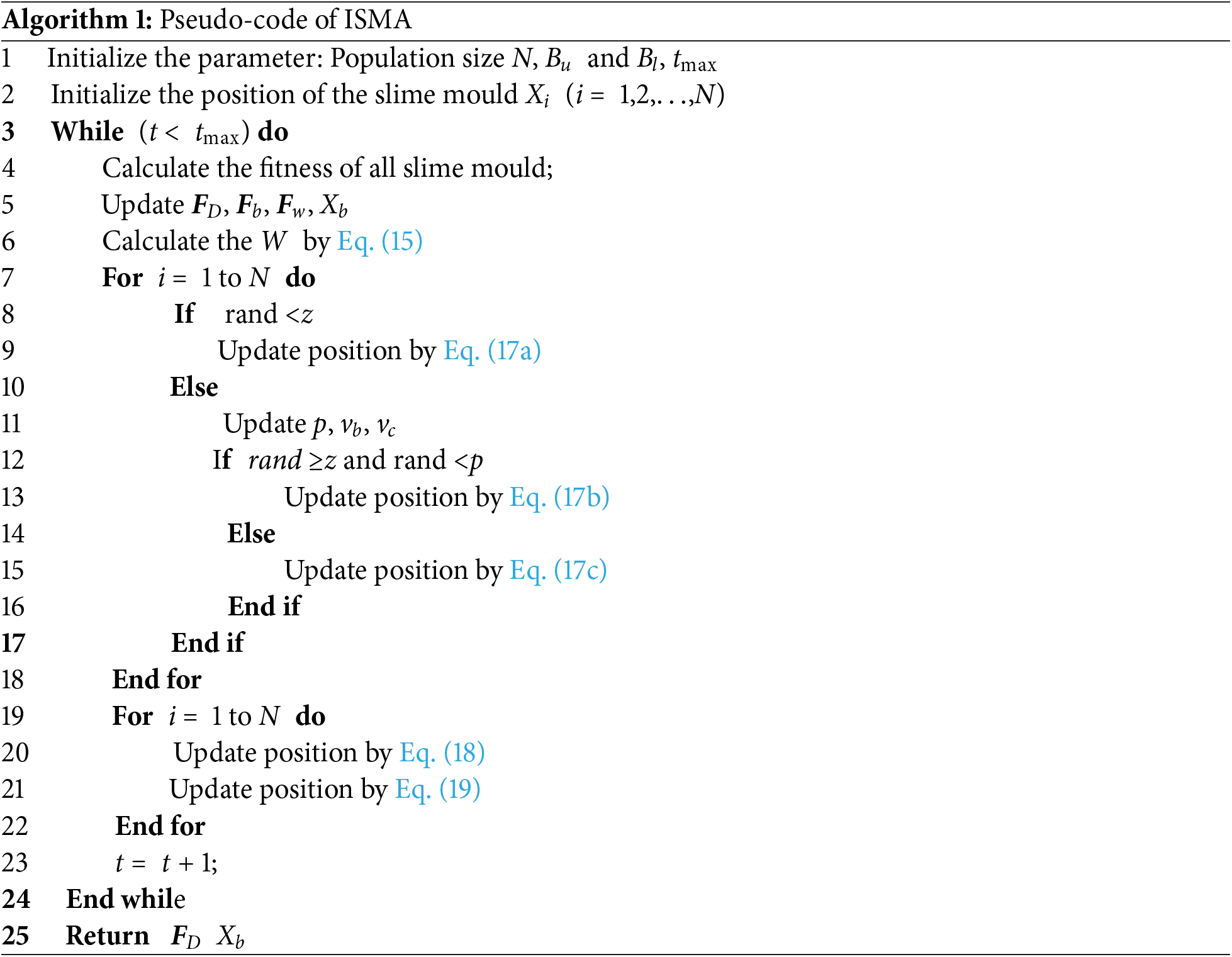
The pseudo code of the ISMA is shown in Algorithm 1.

Compared with the improvements in Reference [36], the difference between this paper and the reference lies in the position update behavior. The method in this paper employs adaptive adjustment of weight coefficients and random positions of individuals to escape from local optima. In contrast, Reference [36] developed an arbitrary average position to enable the algorithm to break free from local optima and explore a broader solution space. Moreover, the ISMA method in this paper takes into account the mutation behavior of the optimal individual to increase the probability of escaping from local optima.

3.3 Details of the Proposed ISMA-VFEEI Method

The aim of the proposed ISMA-VFEEI method is to construct a VF surrogate model by efficiently using the LF and HF samples, where the ISMA is provided to obtain sufficiently accurate optimal results when reducing the computational cost. The flowchart of the proposed ISMA-VFEEI method is shown in Fig. 1.

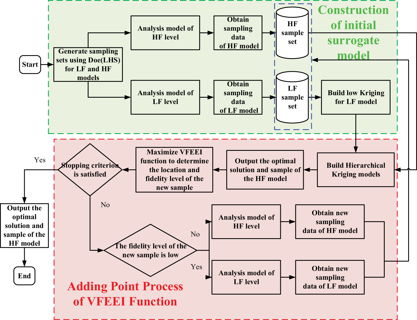
Figure 1: Flowchart of the proposed ISMA-VFEEI method

The specific steps of the proposed ISMA-VFEEI method are elaborated as follows.

Step 1: The Design of Experiment (DoE) method is used to generate the initial HF and LF sample points separately. For example, HF samples xh={x1h,x2h,⋯,xnhh} and LF samples xl={x1l,x2l,⋯,xnll} are generated using Latin Hypercube Sampling (LHS).

Step 2: The design samples are imported into the corresponding models with different levels of fidelity and the response values fh={f1h,f2h,⋯,fnhh} and fl={f1l,f2l,⋯,fnll} are output.

Step 3: A Hierarchical Kriging model is built based on the current set of samples.

Step 4: The proposed ISMA method is used to obtain the minimum of the high-fidelity model and output the location and response values of the minimum sample.

Step 5: The proposed ISMA method of maximizing the VFEEI function is used to determine the updated point and the corresponding level of fidelity.

Step 6: The termination condition is judged in each iteration. The total computational cost is considered, and the computational cost of the LF samples is converted to the computational cost of the HF samples and the expression for the total cost is

{|y^min−yreal|≤εCtotal≥CmaxJ≥Jmax(20)

where y^min represents the predicted optimal solution in the optimization process and yreal is the known optimal solution, ε is the allowed minimum error, Cmax is the allowed maximum computational cost and Jmax is the maximum number of points allowed to be added. For engineering problems, the maximum computational cost and the maximum number of points to be added are set as termination conditions.

If this condition is met, the algorithm switches to step 9, otherwise, it returns to step 7. We will explicitly state that if the maximum limits for computational cost and the number of samples are reached and the error is still greater than the allowed range, the algorithm will proceed with the final assessment of performance. In this scenario, we recommend that after the calculation is terminated, the sample points of the initial model should be increased and the calculation should be carried out again until the requirements of the algorithm are met.

Step 7: The updated sample is imported into the corresponding models with different levels of fidelity and the response values of the updated samples are outputted.

Step 8: Add the updated sample to the HF or LF sample set and re-establish the Hierarchical Kriging model. Return to Step 3.

Step 9: If the termination condition is satisfied, the optimal solution and the corresponding sample position are outputted using the ISMA algorithm.

4  Examples and Discussions

4.1 Validation of ISMA

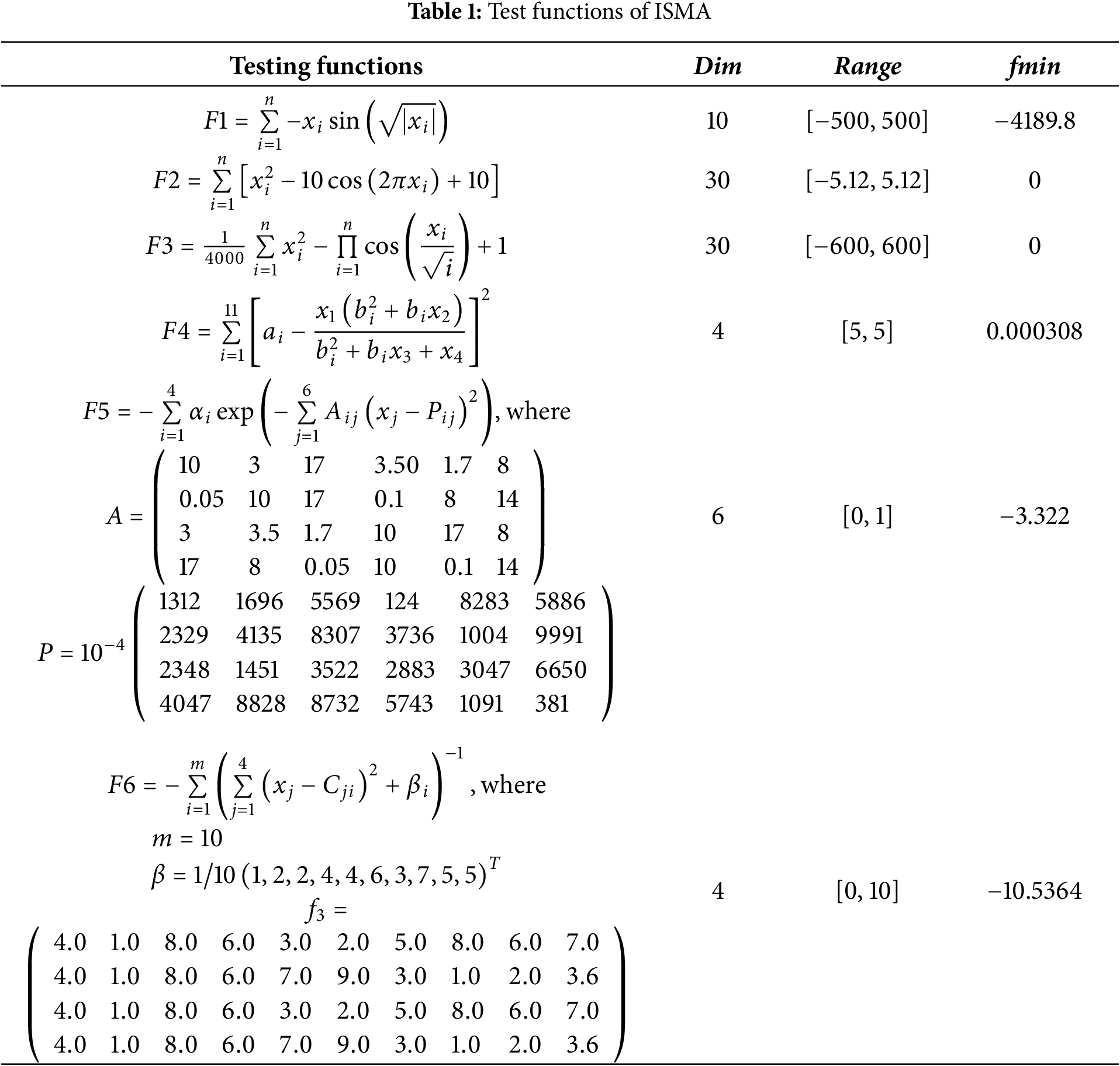
In order to verify the effectiveness of the ISMA algorithm, six testing functions are employed and compared to the original SMA algorithm. The testing functions from CEC2005 and reference [31]. The specific information of the testing functions is shown in Table 1.

For a comparison with other methods, the population size N = 30, dimension Dim = 10 and maximum number of iterations tmax = 1000 are set. 30 times are run independently on each testing function, and the average and standard deviation are provided in Table 2.

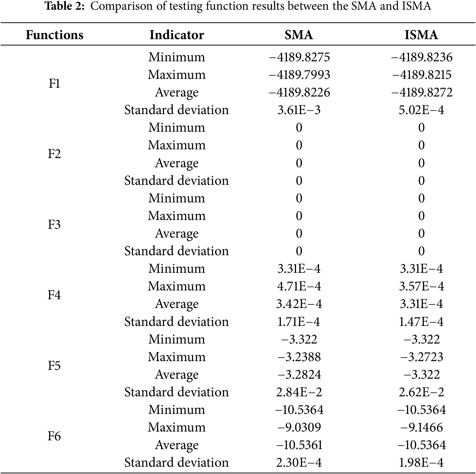
From Table 2, we can see that ISMA can obtain better results compared to the original SMA algorithm, both from the mean and standard deviation. In order to compare the convergence speed and accuracy of each algorithm more intuitively, the average convergence curves of the testing functions are presented in Fig. 2. From Fig. 2, we can see that the convergence speed of the ISMA is also better than that of the original SMA.

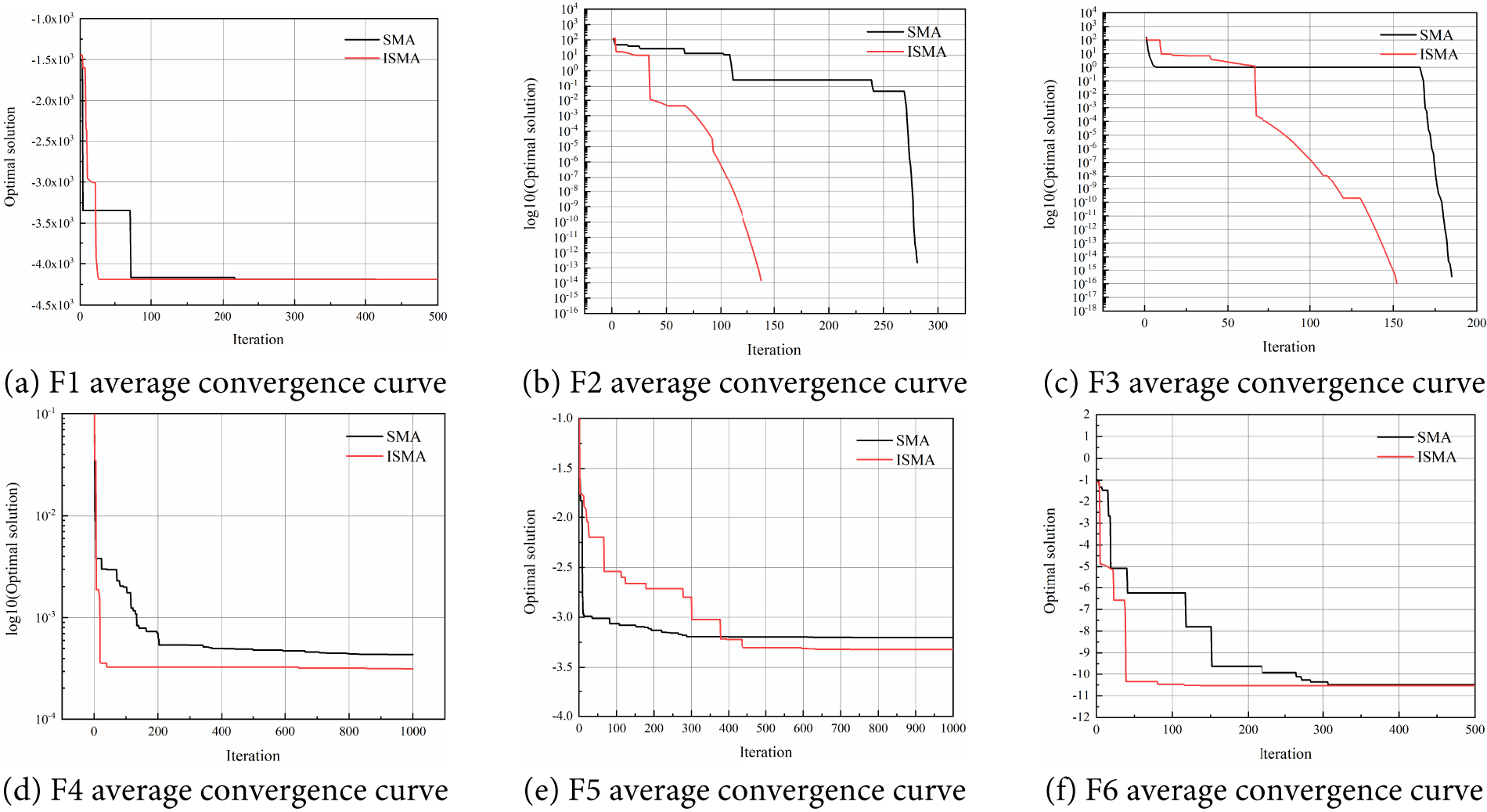
Figure 2: Average convergence curve of the test functions

To further evaluate the performance of ISMA, this paper employs the Wilcoxon rank-sum test to examine whether there is a significant difference between the performance of ISMA and SMA. The significance level is set at 0.05, and the optimization results from 30 runs of all algorithms are used as samples. When the p-value of the test is greater than 0.05, it indicates that there is no significant difference between the results of the two algorithms; otherwise, a significant difference exists. Table 3 presents the results of the Wilcoxon rank-sum test between ISMA and the comparison algorithms.

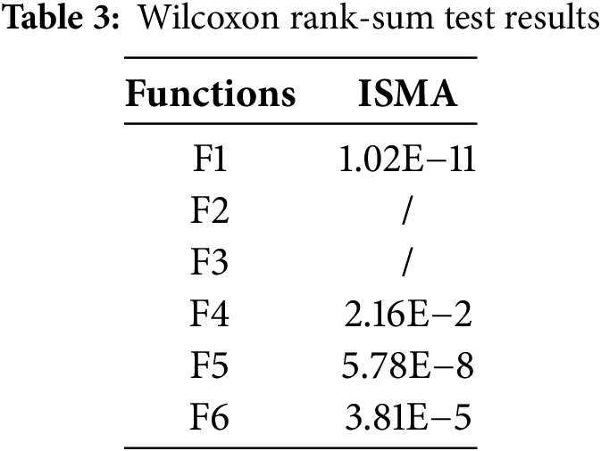
As shown in Tables 2 and 3, ISMA outperforms ESMA and SMA on four test functions. Therefore, ISMA demonstrates statistically significant superiority in performance. The experimental results indicate that the proposed ISMA in this paper has significantly improved convergence speed, solution accuracy, and robustness.

4.2 An Illustrative Example of ISMA-VFEEI

A one-dimensional numerical case is applied to illustrate the detailed procedure of the method proposed in this subsection. The mathematical model is

{minf2(x)=(6x−2)2sin⁡(12x−4)f1(x)=0.5f2(x)+10(x−0.5)−5s.t.x∈[0,1](21)

where f2(x) denotes the HF analytical function and f1(x) denotes the LF analytical function. The theoretical optimal solution is x∗=0.75725 with the optimal functional value. The computational cost ratio between the HF and LF models is assumed to be 4. Termination condition ε = 0.01.

First, two initial sample sets containing three HF sample points xh = {0.02198, 0.53247, 0.99455} and six LF sample points xl = {0.04996, 0.26578, 0.43828, 0.62033, 0.80575, 0.98358} are generated. Based on the initial sampling points, an initial VF metamodel is built. After the initial VF metamodel is built, the refinement process of the HF model using the proposed method is shown in Fig. 3. The left graph of Fig. 3 shows the iterative process of the surrogate model and the right side of Fig. 3 shows the distribution of the corresponding VFEEI functions in the design space. In the left panel of Fig. 3, the red solid curve denotes the true high-fidelity function, while the blue solid curve denotes the true low-fidelity function. The red dashed curve shows the surrogate’s high-fidelity prediction, and the blue dashed curve shows its low-fidelity prediction. Pink hollow triangles mark the high-fidelity sample locations, and green hollow squares indicate the low-fidelity sample locations. In the right panel of Fig. 3, the red solid curve depicts the high-fidelity VFEEI acquisition function, and the blue solid curve depicts the low-fidelity VFEEI acquisition function. Pink hollow triangles denote the maxima of the high-fidelity VFEEI, while green hollow squares denote the maxima of the low-fidelity VFEEI. During the optimization process, the sizes of the VFEEI functions of these two samples are used to determine whether they should be added to the initial sample set.

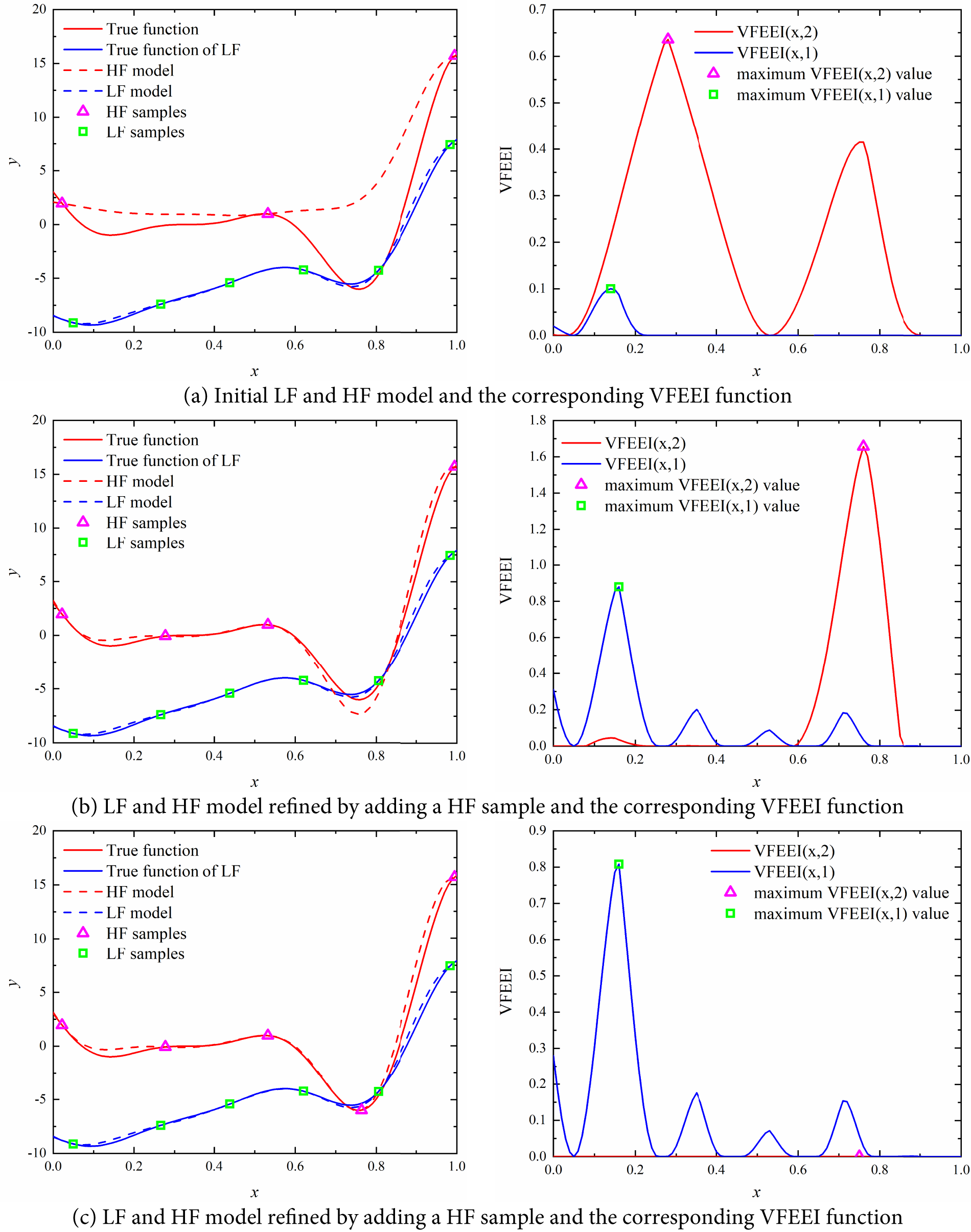
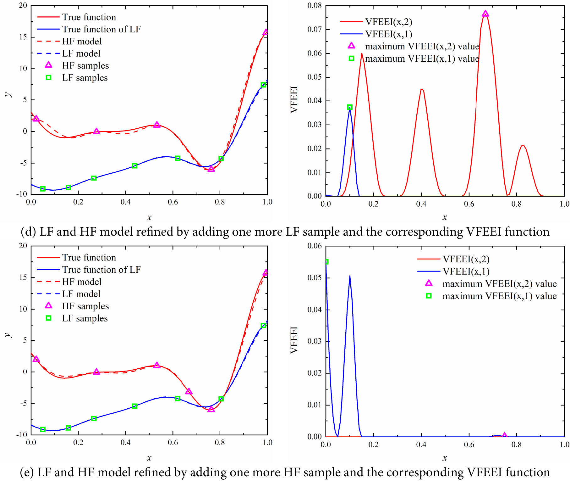
Figure 3: Refinement process of optimization based on the proposed VFEEI

From Fig. 3a, we can see that the LF surrogate model is not accurate but has a similar trend compared to the HF model, and the maximum value of the VFEEI function of the HF model is much larger than that of the HF model. When an HF sample in the second cycle is added, the accuracy can be improved greatly than the LF added. For this example, the iteration is terminated in the fifth cycle. The optimal solution is obtained by using the ISMA algorithm. For high-fidelity models, when the fitting samples cannot represent the overall trend of the function, global exploration will be conducted through the VFEEI function, as illustrated in Fig. 3b. Conversely, when the fitting samples can represent the overall trend of the function but the local prediction performance is poor, the VFEEI function will focus on the local development, as shown in Fig. 3c. After two iterations, the final high-fidelity function surrogate model is shown in Fig. 3e.

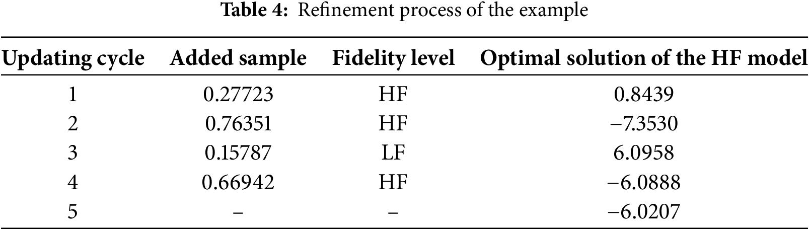
The optimization process is provided in Table 4. When one LF sample and three HF samples are added, the global optimal solutions can be obtained and the last iteration (the fifth cycle) of the surrogate model is provided in Fig. 3e. From the results, we can see that the proposed method can build a highly accurate VF surrogate model by combining the LF and HF samples.

To further verify the effectiveness of the proposed VFEEI function, the impact of the sample distance function on global optimization is investigated next. In this case, the sample distance function is removed from the VFEEI function (referred to as VFEEI-D), and optimization is performed based on this modified function. The final comparative results are shown in Fig. 4.

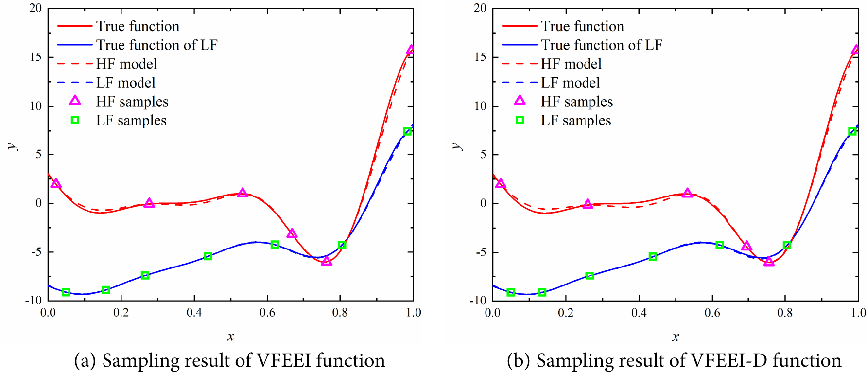
Figure 4: Comparison chart of sampling results from different acquisition functions

As shown in Fig. 4, the sampling points obtained using the VFEEI-D function tend to cluster, especially near the minimum value. The high-fidelity sampling points obtained using the VFEEI function exhibit significantly better discreteness compared to those obtained using the VFEEI-D function. This conclusion also applies to the low-fidelity sampling process, particularly in the region near 0.1. Additionally, in areas not covered by high-fidelity samples, such as near 0.1 and 0.4, it is evident that the fitting effect of the high-fidelity function in Fig. 4b is slightly worse than that in Fig. 4a. These analyses fully demonstrate that the sample distance function is highly sensitive to the entire sampling process and plays a crucial role in the prediction accuracy of multi-fidelity models.

4.3 Testing Functions of ISMA-VFEEI

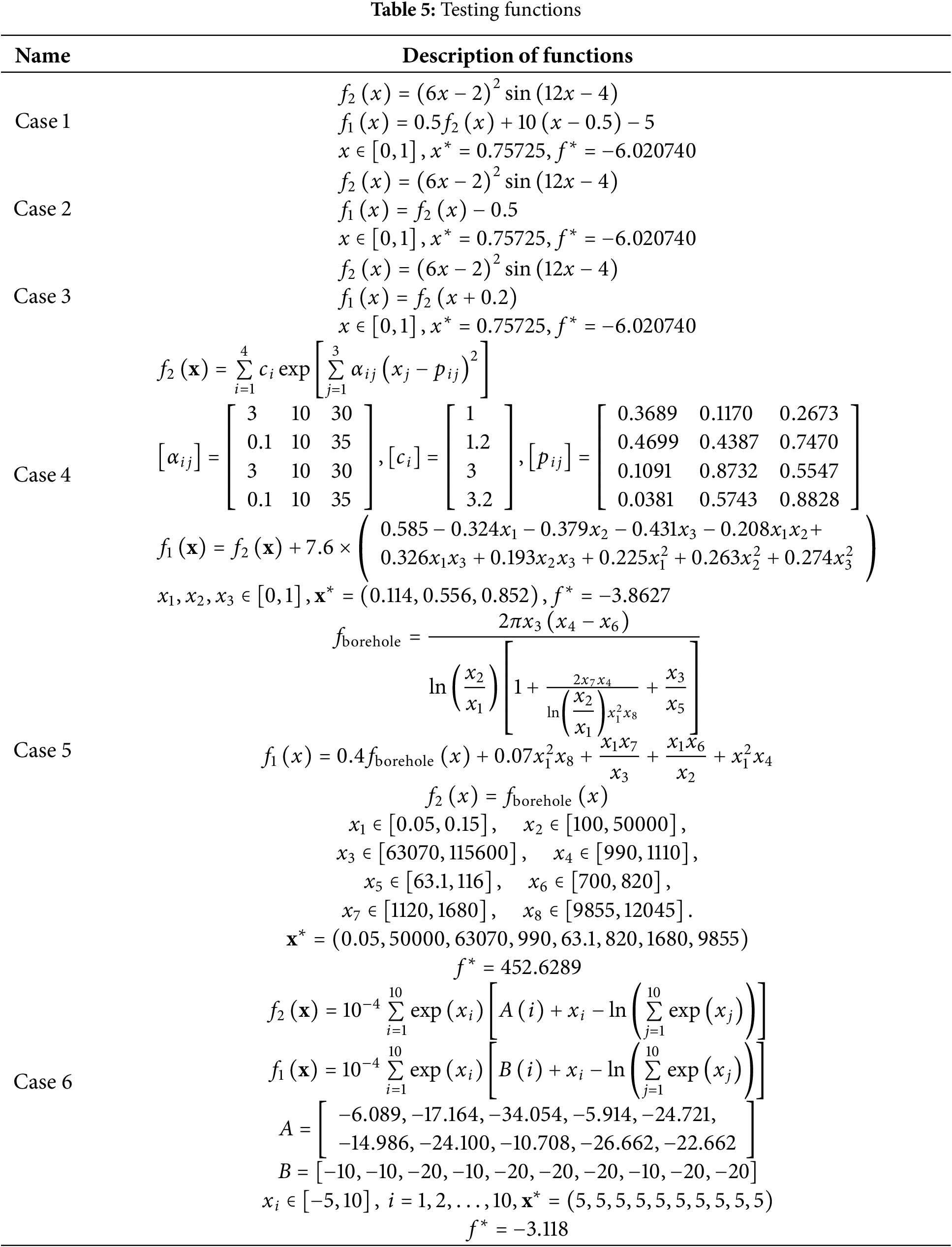
In this subsection, six commonly used numerical examples are used to illustrate the effectiveness and efficiency of the proposed ISMA-VFEEI method. Especially, the testing functions in cases 5 and 6 are highly nonlinear. These test functions were modified from references [14,42]. The expressions of the testing functions are shown in Table 5. The computational cost ratio between HF evaluation and LF evaluation is set to 4 for all testing examples.

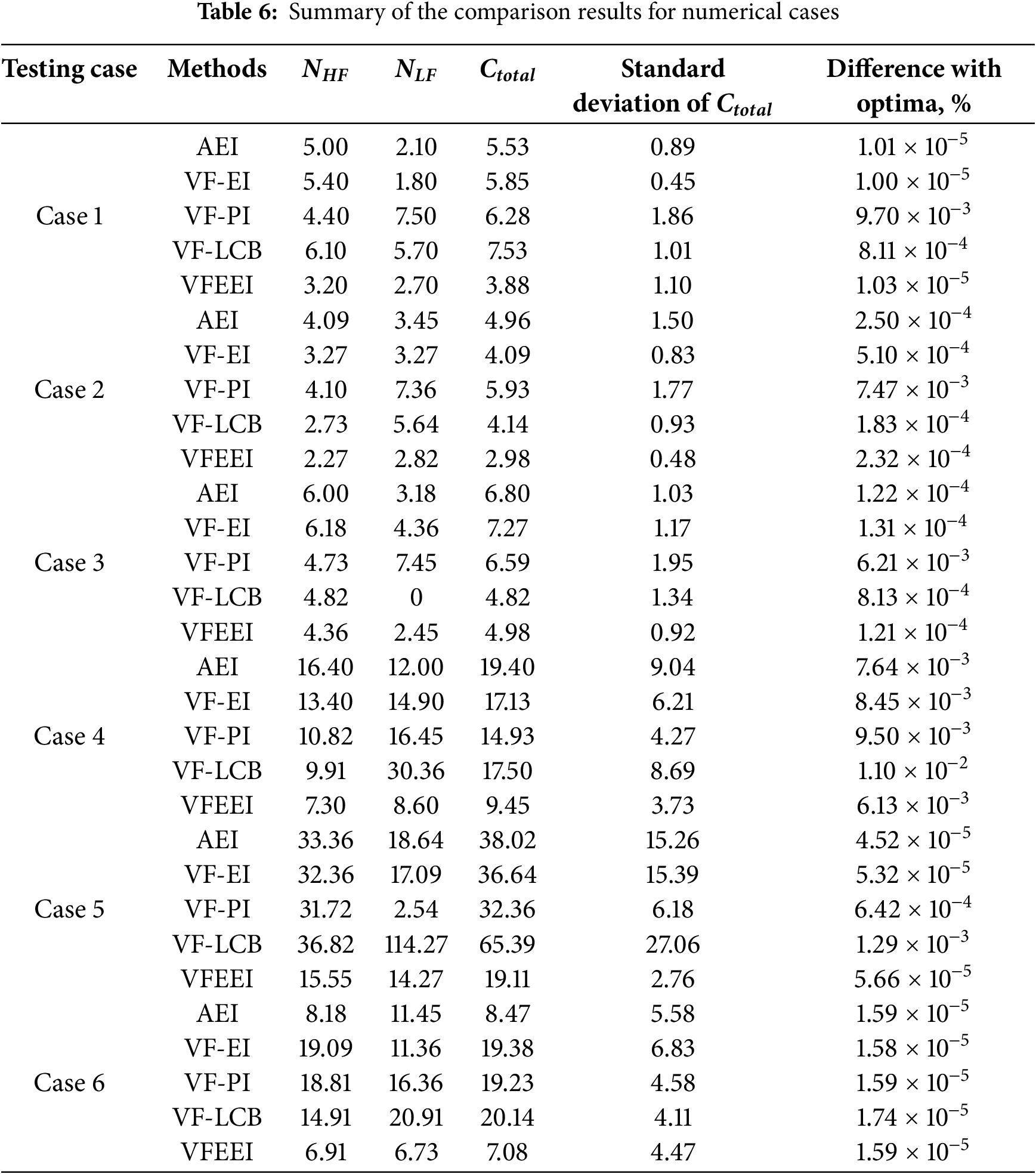
In the first five testing functions, the initial HF and LF samples are set to 3d and 6d, respectively, while in the last testing case, the initial HF and LF samples are set to 10d and 20d, respectively, where d denotes the dimension of the design variables. Considering the randomness of the LHS and ISMA methods, 10 runs are performed for each method. NHF and NLF denote the number of function calls for the HF and LF models, respectively. In order to measure the robustness of each method, the standard deviation of the total cost is used. The relative error is calculated to describe the computational accuracy. The compared methods used here are the AEI [12], the VF-EI [14], the VF-LCB [17] and the VF-PI [24]. The results are shown in Table 6. All acquisition functions are computed using ISMA.

Compared with the original EI, VFEEI extends EI to handle multi-fidelity data and additionally considers sample distance and computational cost. Compared with VFEEI, AEI further takes into account the correlation between data of different fidelities. Compared with VF-EI, VFEEI handles the original EI differently; in VF-EI, the same high-fidelity function prediction value is used for EI at different fidelities. All the aforementioned methods are based on EI. In contrast, VF-PI and VF-LCB are improved versions of the probability of improvement function and the low confidence bound function, respectively.

The comparison of different methods reveals significant reductions in both high-fidelity (HF) computation costs and total costs across the six examples. Specifically, compared to the AEI method, the HF calculation cost is reduced to 55% (improved by 36%), and the total cost to 51% (improved by 30%). These reductions indicate the effectiveness of the proposed method in improving computational efficiency.

In comparison with the VF-EI method, the HF calculation cost is reduced by up to 64%, with a corresponding decrease in total cost ranging from 27% to 63%. This shows a notable improvement in computational efficiency, particularly in the cases where the cost reduction is most pronounced.

The VF-PI method also shows a reduction in HF calculation costs (8% to 51%) and total costs (27% to 63%). However, the improvements are less consistent than those observed when compared to the VF-EI method, suggesting that the VF-EI method may offer a more stable advantage in terms of overall computational savings.

When compared to the VF-LCB method, the reductions in HF calculation costs are substantial, ranging from 10% to 58%, while the total cost reduction varies from −3% to 71%. The negative value for the total cost in one of the examples indicates that, in some cases, the VF-LCB method might perform better than the proposed method in terms of total cost, but the proposed method generally shows superior efficiency across the majority of examples.

In summary, while all methods demonstrate varying degrees of improvement, the proposed method consistently outperforms the AEI, VF-EI, VF-PI, and VF-LCB methods in reducing computational costs, particularly for high-fidelity calculations, making it a more efficient approach for the examples studied. To testify to the robustness of all the methods, the standard deviation of the total costs is also provided in Table 5. For an intuitive comparison, a box plot of the total costs for all methods in the six different cases is described in Fig. 5. We can see that all methods exhibit the desired robustness. The robustness of the proposed method is less than the other methods only in Case 1, but better than the other methods in other cases.

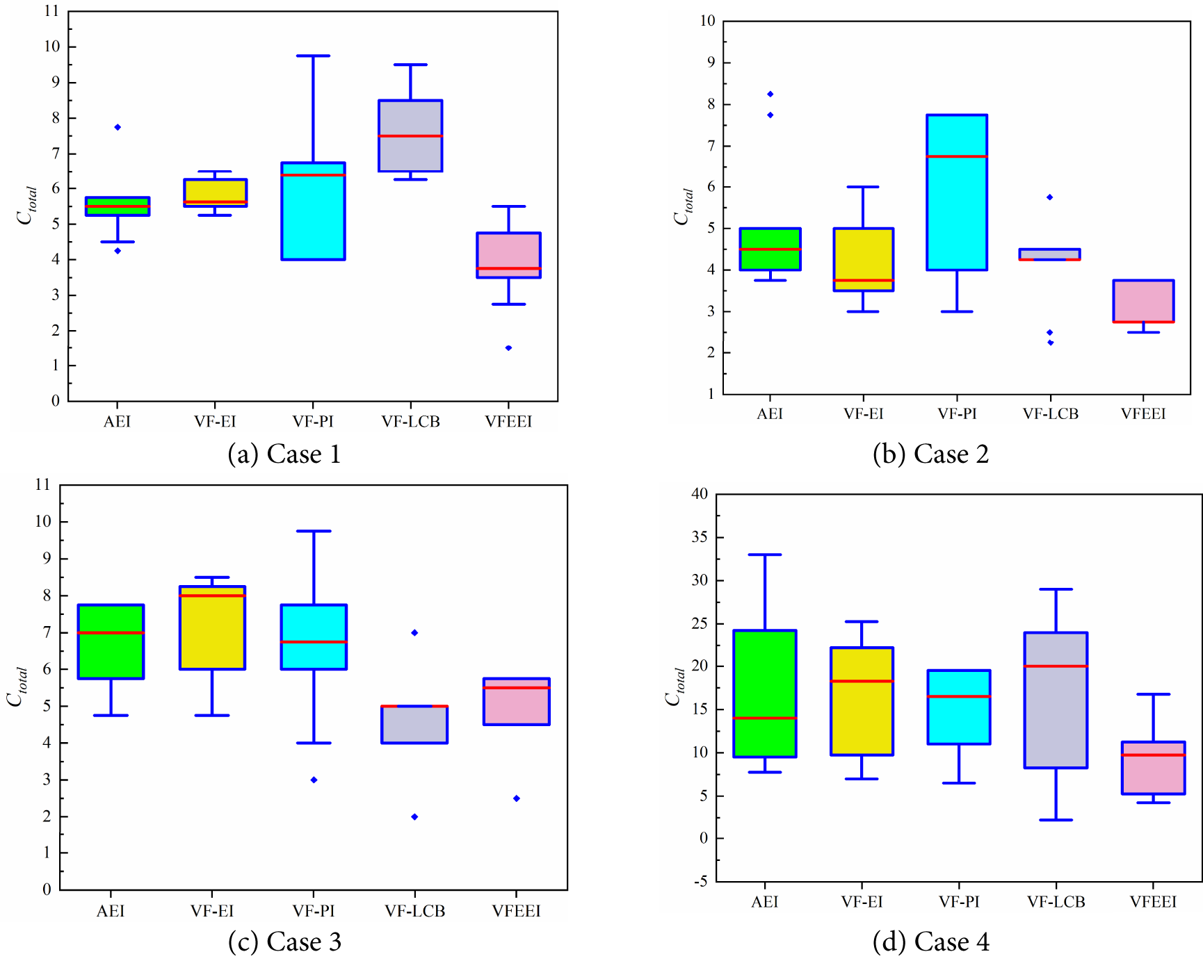
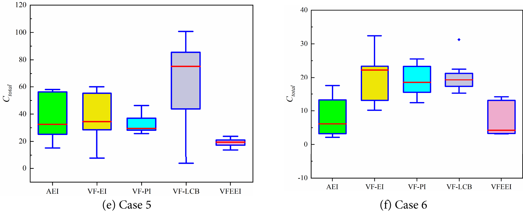
Figure 5: Comparison results of different cases for the proposed VFEEI method and other methods

The results of the Wilcoxon rank-sum test for different methods are shown in Table 7. Among the six test cases, all Wilcoxon rank-sum test p-values are greater than 0.05, indicating that there are no significant differences between the optimization results obtained using VFEEI and those obtained using the other four methods. This is because, in this subsection, the primary focus is on testing the computational effects of different acquisition functions, and the convergence criterion during the optimization process is the optimization precision error within a fixed cost range. Therefore, all methods are able to obtain the optimal solution. In this example, the Wilcoxon rank-sum test is used to compare the statistical results of the optimal solutions computed by different acquisition functions.

4.4 Engineering Example

With the quick development of the high-speed railway, the safety of the Electric Multiple Unit (EMU) becomes more and more important as the speed increases. As one of the important structural components of the EMU, the sanding device can improve the adhesion coefficient between the wheel and rail by sanding to ensure the smooth operation of the EMU in harsh weather such as rain and snow, which can prevent wheelset idling and vehicle taxiing, and effectively avoid the occurrence of wheel rub fault. This section mainly conducts static strength analysis on the sanding device.

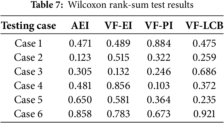
The entire structure of the sanding device is made of 5-5083-H111 aluminium alloy. Its modulus of elasticity is 7 × 104 MPa, density is 2700 kg/m3, Poisson’s ratio is 0.33, yield strength is 139 MPa, and its main structural components include sand box, sand spreader, hoisting structure, sand inlet pipe, etc. The structural composition of the sanding device is shown in Fig. 6.

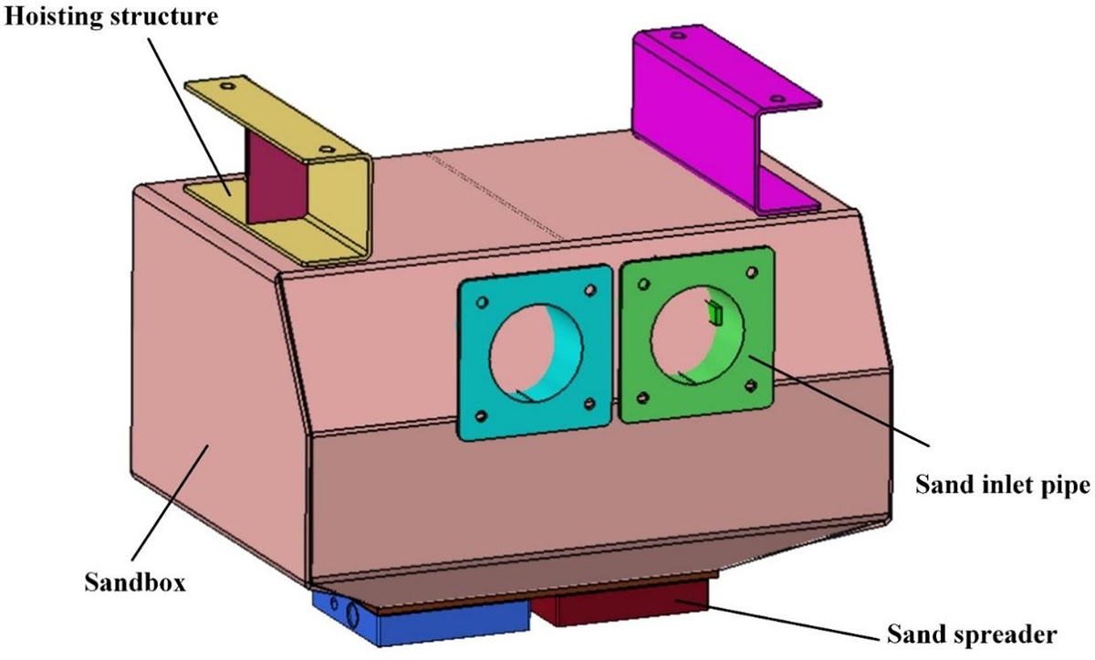
Figure 6: The structural composition of the sanding device

The sanding device is connected to the rest of the rolling stock by a hoisting structure. The constraints of the sanding device are established at the location of the bolt holes in the hoisting structure of the sand spreader, which constrains six directions of freedom, limiting in-plane movement and rotation in space. Also, an acceleration condition with a longitudinal acceleration of 5 g and a vertical acceleration of 1 g was determined as the working condition, where g is the acceleration of gravity. The finalised key parameter locations and constraint locations for the sanding device are shown in Fig. 7. The symbols and thicknesses of the key locations of the sanding device are summarised in Table 8.

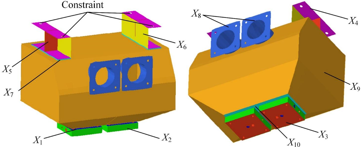
Figure 7: Location of key parameters and constraint positions of the sanding device

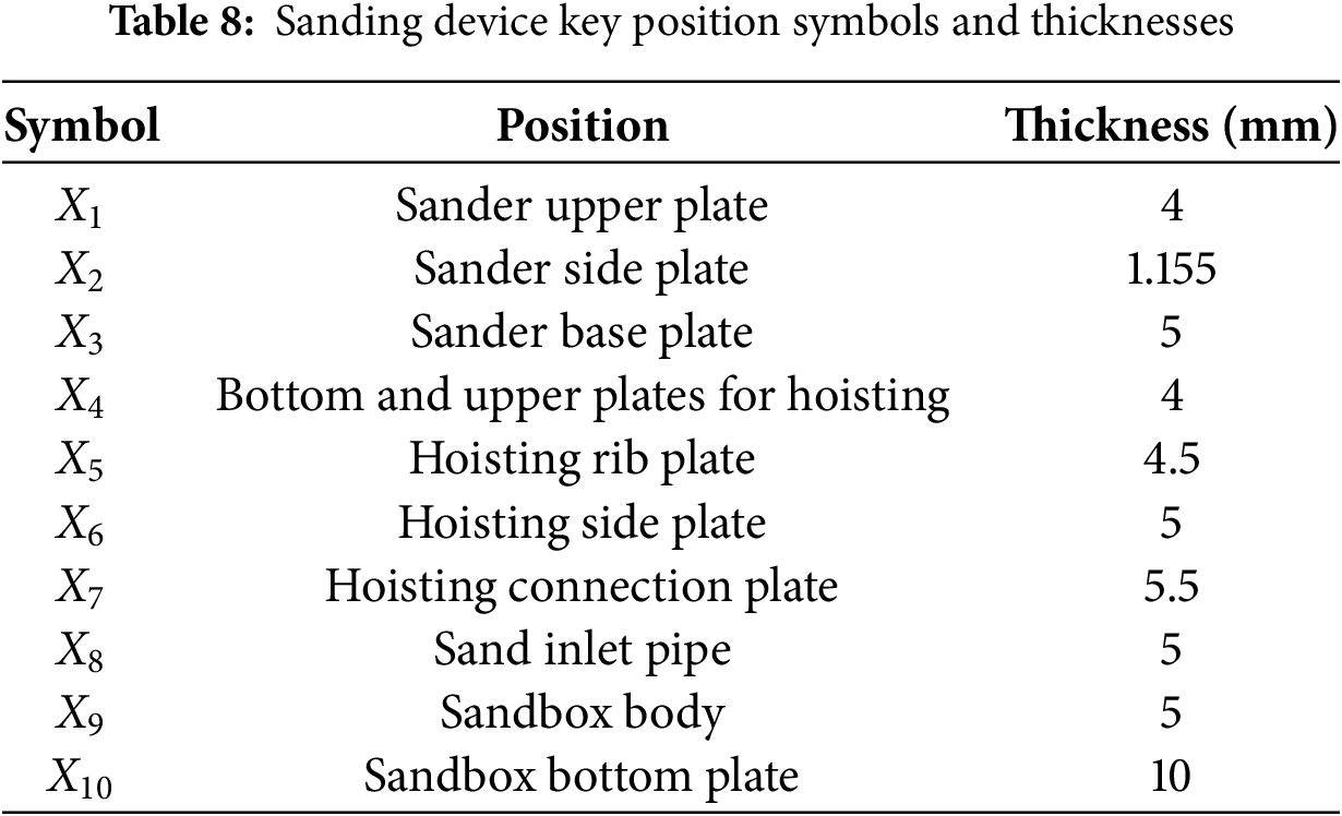
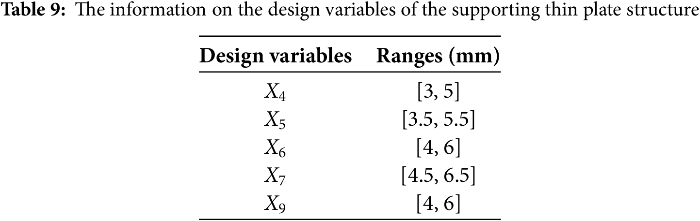
In order to determine the sensitive parameters on the stress and mass of the sanding device from X1~X10, the sensitivity analysis is performed and the results are shown in Fig. 8. From Fig. 8, we can see X4, X5, X6, X7, X9 are sensitive parameters and the information on the sensitive parameters is provided in Table 9.

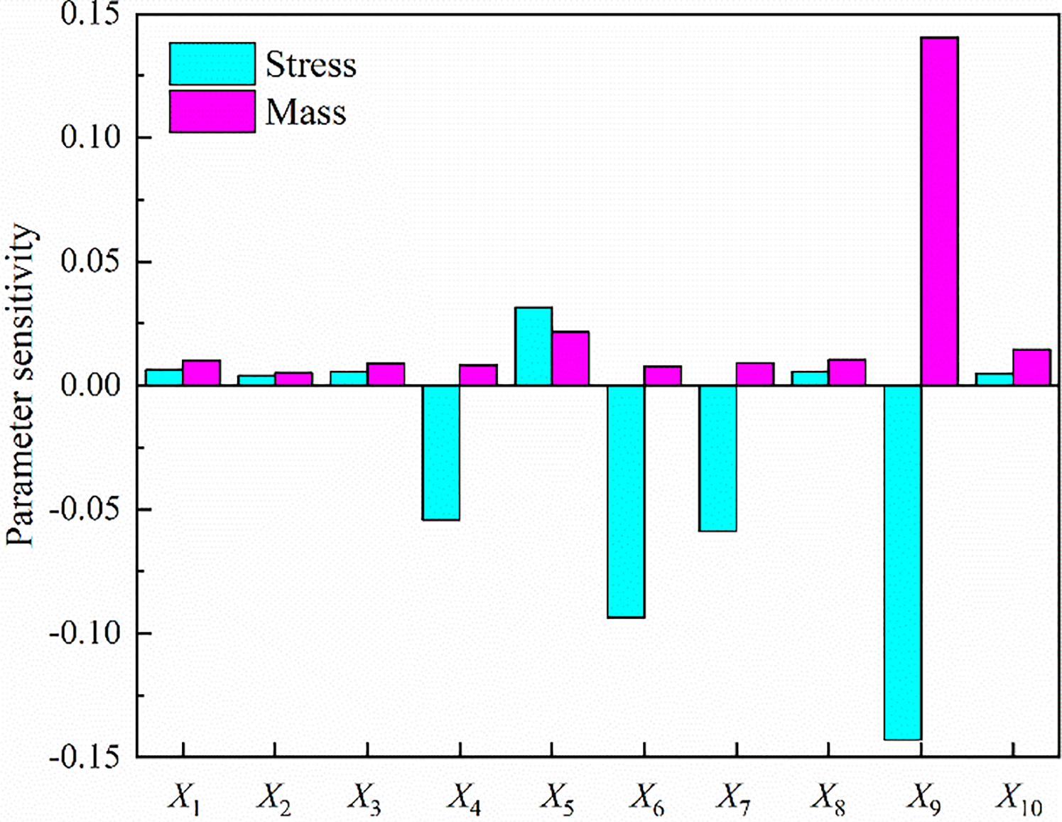
Figure 8: Sensitivity analysis on the stress and mass

Then the optimization model can be expressed by

Find x={X4,X5,X6,X7,X9}minf=LS(X4,X5,X6,X7,X9)139+LM(X4,X5,X6,X7,X9)0.02683s.t.3≤X4≤5,3.5≤X5≤5.5,4≤X6,X9≤6,4.5≤X7≤6.5(22)

where LS represents the performance function on stress and LM represents the performance function on mass, which are both obtained from surrogate modelling; 139 MPa represents the yield stress and 0.02683 represents the quality of the original model.

A simulation model with approximately 4343 elements was chosen as the LF model, while the HF simulation model had approximately 7004 elements. The mesh and corresponding simulation results are shown in Fig. 9. The single computation time of the HF model is 62.5682 s, while the LF model is 25.2731 s. The computational time for the HF simulation model is approximately 2.5 times longer than that of the LF simulation model. Therefore, the cost ratio was set to 2.5.

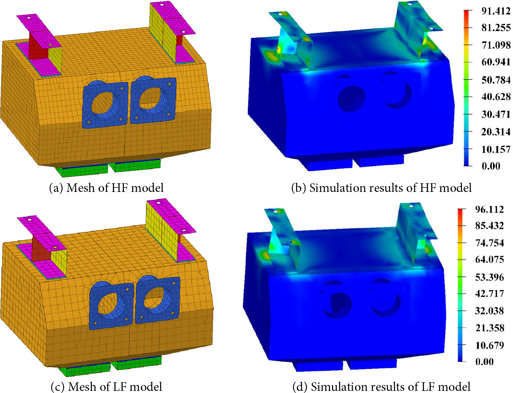
Figure 9: The mesh and corresponding simulation results of the sanding device

The proposed method and other methods are applied to solve this engineering problem. The optimization starts with 5 HF initial sampling points and 10 LF initial sampling points. The termination condition for the optimization is set to the total computational cost, which is determined to be no more than the computational time of the 20 HF simulation models. The optimal results for the design variables for each method are given in Table 10. Table 11 summarizes the optimization target results and computational costs for all methods.

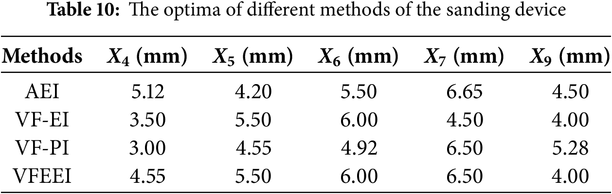
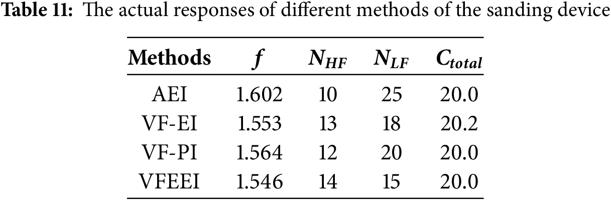
As can be seen in Tables 10 and 11, all methods obtained the optimised design solution while satisfying the termination criterion. Among the four methods, the VFEEI obtained the globally optimal solution with the Ctotal of 20.0, which is reduced by 1.0% compared with the VF-EI method. From the optimization results, VFEEI achieved the minimum value of optimization, which was reduced by 3.50%, 0.45%, and 1.15% compared with AEI, VF-EI, and VF-PI, respectively. The finite element simulation results of the optimal solution are provided in Fig. 10 from the proposed method.

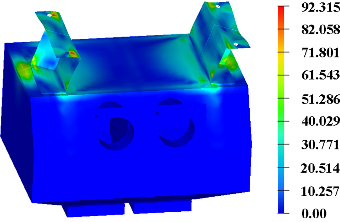
Figure 10: Simulation results of the optimum model by the proposed VFEEI method

5  Conclusion

In this paper, a novel VF Kriging surrogate model-based global optimization method for black-box function (ISMA-VFEEI) is proposed based on the Hierarchical Kriging model. In the proposed method, the VFEEI sampling function is developed to properly select new samples with low and high fidelity to update the surrogate model so that it obtains the global optimal solution. In addition, to improve the accuracy and efficiency of the optimization during the sample updating procedure, an improved slime mould algorithm (ISMA) is proposed to obtain the optimal value of the VFEEI function. Finally, a computational framework applicable to the proposed method is constructed.

The main conclusions can be summarized as follows: (1) ISMA-VFEEI allows for an objective balancing of global exploration and local exploitation to find the global optimal solution, and also achieves robust results by consuming fewer computational resources. (2) Six numerical examples illustrate the advantages of the proposed method in terms of computational cost and robustness. The quartile spacing of the proposed method is smaller than that of the other methods, which demonstrates the better robustness of the proposed method. (3) The optimization of the sanding device verifies the engineering application value of this method. Compared with the VF-EI and AEI methods, this method achieved better results with fewer calculations.

In our future work, the method proposed in this paper can be extended to conduct uncertainty optimization to be more applicable for complex engineering problems.

Acknowledgement: This work was funded by National Natural Science Foundation of China; Special Program of Huzhou; Projects of Huzhou Science and Technology Correspondent; Guangdong Basic and Applied Basic Research Foundation.

Funding Statement: This work was funded by National Natural Science Foundation of China (grant No. 52405255); Special Program of Huzhou (grant No. 2023GZ05); Projects of Huzhou Science and Technology Correspondent (grant No. 2023KT76); Guangdong Basic and Applied Basic Research Foundation (grant No. 2025A1515010487).

Author Contributions: Yi Guan: conceptualization, methodology, writing—original draft preparation; Pengpeng Zhi: supervision, project administration, funding acquisition; Zhonglai Wang: supervision, writing—review and editing. All authors reviewed the results and approved the final version of the manuscript.

Availability of Data and Materials: The data that support the findings of this study are available from the corresponding authors upon reasonable request.

Ethics Approval: Not applicable.

Conflicts of Interest: The authors declare no conflicts of interest to report regarding the present study.

References

1. Yang H, Hong SH, Wang Y. A sequential multi-fidelity surrogate-based optimization methodology based on expected improvement reduction. Struct Multidiscip Optim. 2022;65(5):153. doi:10.1007/s00158-022-03240-x. [Google Scholar] [CrossRef]

2. Biagiola SI, Figueroa JL. Wiener and Hammerstein uncertain models identification. Math Comput Simul. 2009;79(11):3296–313. doi:10.1016/j.matcom.2009.05.004. [Google Scholar] [CrossRef]

3. Harkin EF, Shen PR, Goel A, Richards BA, Naud R. Parallel and recurrent cascade models as a unifying force for understanding subcellular computation. Neuroscience. 2022;489:200–15. doi:10.1016/j.neuroscience.2021.07.026. [Google Scholar] [PubMed] [CrossRef]

4. Zhang J, Chowdhury S, Messac A. An adaptive hybrid surrogate model. Struct Multidiscip Optim. 2012;46(2):223–38. doi:10.1007/s00158-012-0764-x. [Google Scholar] [CrossRef]

5. Zhou Q, Shao X, Jiang P, Zhou H, Shu L. An adaptive global variable fidelity metamodeling strategy using a support vector regression based scaling function. Simul Model Pract Theory. 2015;59(3):18–35. doi:10.1016/j.simpat.2015.08.002. [Google Scholar] [CrossRef]

6. Tyan M, Nguyen NV, Lee JW. Improving variable-fidelity modelling by exploring global design space and radial basis function networks for aerofoil design. Eng Optim. 2015;47(7):885–908. doi:10.1080/0305215X.2014.941290. [Google Scholar] [CrossRef]

7. Liu Y, Collette M. Improving surrogate-assisted variable fidelity multi-objective optimization using a clustering algorithm. Appl Soft Comput. 2014;24:482–93. doi:10.1016/j.asoc.2014.07.022. [Google Scholar] [CrossRef]

8. Li X, Qiu H, Jiang Z, Gao L, Shao X. A VF-SLP framework using least squares hybrid scaling for RBDO. Struct Multidiscip Optim. 2017;55(5):1629–40. doi:10.1007/s00158-016-1588-x. [Google Scholar] [CrossRef]

9. Viana FAC, Simpson TW, Balabanov V, Toropov V. Special section on multidisciplinary design optimization: metamodeling in multidisciplinary design optimization: how far have we really come? AIAA J. 2014;52(4):670–90. doi:10.2514/1.j052375. [Google Scholar] [CrossRef]

10. Xiao M, Zhang G, Breitkopf P, Villon P, Zhang W. Extended Co-Kriging interpolation method based on mul-ti-fidelity data. Appl Math Comput. 2018;323(4):120–31. doi:10.1016/j.amc.2017.10.055. [Google Scholar] [CrossRef]

11. Han ZH, Görtz S. Hierarchical Kriging model for variable-fidelity surrogate modeling. AIAA J. 2012;50(9):1885–96. doi:10.2514/1.j051354. [Google Scholar] [CrossRef]

12. Huang D, Allen TT, Notz WI, Miller RA. Sequential Kriging optimization using multiple-fidelity evaluations. Struct Multidiscip Optim. 2006;32(5):369–82. doi:10.1007/s00158-005-0587-0. [Google Scholar] [CrossRef]

13. Xiong Y, Chen W, Tsui KL. A new variable-fidelity optimization framework based on model Fusi on and objec-tive-oriented sequential sampling. J Mech Des. 2008;130(11):111401. doi:10.1115/1.2976449. [Google Scholar] [CrossRef]

14. Zhang Y, Han ZH, Zhang KS. Variable-fidelity expected improvement method for efficient global optimization of expensive functions. Struct Multidiscip Optim. 2018;58(4):1431–51. doi:10.1007/s00158-018-1971-x. [Google Scholar] [CrossRef]

15. Liu Y, Chen S, Wang F, Xiong F. Sequential optimization using multi-level cokriging and extended expected im-provement criterion. Struct Multidiscip Optim. 2018;58(3):1155–73. doi:10.1007/s00158-018-1959-6. [Google Scholar] [CrossRef]

16. Han Z, Xu C, Zhang L, Zhang Y, Zhang K, Song W. Efficient aerodynamic shape optimization using varia-ble-fidelity surrogate models and multilevel computational grids. Chin J Aeronaut. 2020;33(1):31–47. doi:10.1016/j.cja.2019.05.001. [Google Scholar] [CrossRef]

17. Jiang P, Cheng J, Zhou Q, Shu L, Hu J. Variable-fidelity lower confidence bounding approach for engineering optimization problems with expensive simulations. AIAA J. 2019;57(12):5416–30. doi:10.2514/1.j058283. [Google Scholar] [CrossRef]

18. Serani A, Pellegrini R, Wackers J, Jeanson CE, Queutey P, Visonneau M, et al. Adaptive multi-fidelity sampling for CFD-based optimisation via radial basis function metamodels. Int J Comput Fluid Dyn. 2019;33(6–7):237–55. doi:10.1080/10618562.2019.1683164. [Google Scholar] [CrossRef]

19. Yi J, Shen Y, Shoemaker CA. A multi-fidelity RBF surrogate-based optimization framework for computationally expensive multi-modal problems with application to capacity planning of manufacturing systems. Struct Multi-discip Optim. 2020;62(4):1787–807. doi:10.1007/s00158-020-02575-7. [Google Scholar] [CrossRef]

20. Shi M, Lv L, Sun W, Song X. A multi-fidelity surrogate model based on support vector regression. Struct Multi-discip Optim. 2020;61(6):2363–75. doi:10.1007/s00158-020-02522-6. [Google Scholar] [CrossRef]

21. He Y, Sun J, Song P, Wang X. Variable-fidelity hypervolume-based expected improvement criteria for mul-ti-objective efficient global optimization of expensive functions. Eng Comput. 2022;38(4):3663–89. doi:10.1007/s00366-021-01404-9. [Google Scholar] [CrossRef]

22. Guo Z, Wang Q, Song L, Li J. Parallel multi-fidelity expected improvement method for efficient global optimization. Struct Multidiscip Optim. 2021;64(3):1457–68. doi:10.1007/s00158-021-02931-1. [Google Scholar] [CrossRef]

23. Cheng J, Lin Q, Yi J. An enhanced variable-fidelity optimization approach for constrained optimization problems and its parallelization. Struct Multidiscip Optim. 2022;65(7):188. doi:10.1007/s00158-022-03283-0. [Google Scholar] [CrossRef]

24. Ruan X, Jiang P, Zhou Q, Hu J, Shu L. Variable-fidelity probability of improvement method for efficient global optimization of expensive black-box problems. Struct Multidiscip Optim. 2020;62(6):3021–52. doi:10.1007/s00158-020-02646-9. [Google Scholar] [CrossRef]

25. Liu Y, Wang S, Zhou Q, Lv L, Sun W, Song X. Modified multifidelity surrogate model based on radial basis func-tion with adaptive scale factor. Chin J Mech Eng. 2022;35(1):77. doi:10.1186/s10033-022-00742-z. [Google Scholar] [CrossRef]

26. Li C, Dong H. A modified trust-region assisted variable-fidelity optimization framework for computationally expensive problems. Eng Comput. 2022;39(7):2733–54. doi:10.1108/ec-08-2021-0456. [Google Scholar] [CrossRef]

27. Tao G, Fan C, Wang W, Guo W, Cui J. Multi-fidelity deep learning for aerodynamic shape optimization using convolutional neural network. Phys Fluids. 2024;36(5):056116. doi:10.1063/5.0205780. [Google Scholar] [CrossRef]

28. Zhang Y, Park S, Simeone O. Multi-fidelity Bayesian optimization with across-task transferable max-value en-tropy search. IEEE Trans Signal Process. 2025;73(1):418–32. doi:10.1109/TSP.2025.3528252. [Google Scholar] [CrossRef]

29. Jariego Pérez LC, Garrido Merchán EC. Towards automatic Bayesian optimization: a first step involving acquisition functions. In: Advances in artificial intelligence. Cham: Springer International Publishing; 2021. p. 160–9. doi:10.1007/978-3-030-85713-4_16. [Google Scholar] [CrossRef]

30. Vincent AM, Jidesh P. An improved hyperparameter optimization framework for AutoML systems using evolu-tionary algorithms. Sci Rep. 2023;13(1):4737. doi:10.1038/s41598-023-32027-3. [Google Scholar] [PubMed] [CrossRef]

31. Li S, Chen H, Wang M, Heidari AA, Mirjalili S. Slime mould algorithm: a new method for stochastic optimiza-tion. Future Gener Comput Syst. 2020;111:300–23. doi:10.1016/j.future.2020.03.055. [Google Scholar] [CrossRef]

32. Ajiboye OK, Ofosu EA, Gyamfi S, Oki O. Hybrid renewable energy system optimization via slime mould algo-rithm. Int J Eng Trends Technol. 2023;7(6):83–95. doi:10.14445/22315381/ijett-v71i6p210. [Google Scholar] [CrossRef]

33. Zhu T, Wan H, Ouyang Z, Wu T, Liang J, Li W, et al. Multi-objective slime mold algorithm: a slime mold approach using multi-objective optimization for parallel hybrid power system. Sens Mater. 2022;34(10):3837. doi:10.18494/sam4020. [Google Scholar] [CrossRef]

34. Singh T. Chaotic slime mould algorithm for economic load dispatch problems. Appl Intell. 2022;52(13):15325–44. doi:10.1007/s10489-022-03179-y. [Google Scholar] [CrossRef]

35. Wu S, Heidari AA, Zhang S, Kuang F, Chen H. Gaussian bare-bone slime mould algorithm: performance opti-mization and case studies on truss structures. Artif Intell Rev. 2023;56(9):1–37. doi:10.1007/s10462-022-10370-7. [Google Scholar] [PubMed] [CrossRef]

36. Devarajah LAP, Ahmad MA, Jui JJ. Identifying and estimating solar cell parameters using an enhanced slime mould algorithm. Optik. 2024;311:171890. doi:10.1016/j.ijleo.2024.171890. [Google Scholar] [CrossRef]

37. Zhang L, Jin G, Liu T, Zhang R. Generalized hierarchical expected improvement method based on black-box functions of adaptive search strategy. Appl Math Model. 2022;106(4):30–44. doi:10.1016/j.apm.2021.12.041. [Google Scholar] [CrossRef]

38. Jones DR, Schonlau M, Welch WJ. Efficient global optimization of expensive black-box functions. J Glob Optim. 1998;13(4):455–92. doi:10.1023/A:1008306431147. [Google Scholar] [CrossRef]

39. Huang H, Liu Z, Zheng H, Xu X, Duan Y. A proportional expected improvement criterion-based multi-fidelity sequential optimization method. Struct Multidiscip Optim. 2023;66(2):30. doi:10.1007/s00158-022-03484-7. [Google Scholar] [CrossRef]

40. Long W, Jiao J, Liang X, Cai S, Xu M. A random opposition-based learning grey wolf optimizer. IEEE Access. 2019;7:113810–25. doi:10.1109/access.2019.2934994. [Google Scholar] [CrossRef]

41. Cao L, Yue Y, Chen Y, Chen C, Chen B. Sailfish optimization algorithm integrated with the osprey optimization algorithm and cauchy mutation and its engineering applications. Symmetry. 2025;17(6):938. doi:10.3390/sym17060938. [Google Scholar] [CrossRef]

42. Hu J, Peng Y, Lin Q, Liu H, Zhou Q. An ensemble weighted average conservative multi-fidelity surrogate modeling method for engineering optimization. Eng Comput. 2022;38(3):2221–44. doi:10.1007/s00366-020-01203-8. [Google Scholar] [CrossRef]