Solving the BBMB Equation in Shallow Water Waves via Space-Time MQ-RBF Collocation

1  Introduction

The dynamics of shallow water waves are governed by various nonlinear evolution equations [1]. These evolution equations hold significant importance in applied mathematics, theoretical physics, and engineering sciences due to their diverse mathematical and physical properties. Among these equations, the Benjamin-Bona-Mahony-Burgers (BBMB) equation represents a significant class of fundamental nonlinear dispersive partial differential equations in mathematical physics [2].

In literature, there are some methods for the analytical solution of the BBMB equation. Typical examples include the multipliers method [3], the Lie symmetry method [4], the Lie symmetry analysis [5], the novel Kudryashov method [6], and so on. However, obtaining exact solutions for the BBMB equation is generally challenging, as only specific cases can be solved analytically [7]. Consequently, numerical methods become essential tools for investigating the physical phenomena described by these nonlinear partial differential equations [8,9].

In literature, several numerical methods have been proposed for solving the BBMB equation. A fourth-order finite difference scheme, which is three-level in time and linear-implicit, was proposed for the BBMB equation [10]. The explicit generalized finite difference scheme was proposed to solve the generalized nonlinear BBMB equation [11]. Xu and Liu investigated a modified Runge–Kutta scheme in terms of a finite difference scheme for the generalized BBMB equation [12]. The iterative kernel-based method, which was proposed by Babak et al. [13], employs positive definite pseudo-spectral kernels and a linearization scheme to solve the nonlinear generalized BBMB equation. A kernel smoothing technique was employed to derive the numerical solution for the BBMB equation [14]. Ngondiep [15] proposed a high-order combined finite element/interpolation approach to simulate the multidimensional nonlinear generalized BBMB equation. The fourth-order backward and compact difference schemes are used for the discretization of the time derivative and spatial derivatives in the BBMB equation [16]. Kanth and Deepika [17] present a non-polynomial spline method for solving the 1-D nonlinear BBMB equation, with its stability analyzed through Von Neumann analysis. Very recently, conforming finite element method [18], nonconforming quadrilateral Quasi-Wilson element [19], the local discontinuous Galerkin (LDG) method [20], the high-order compact finite difference scheme [21], the fully-discrete mixed finite element method [22], the linearized Crank-Nicolson scheme in combination with the virtual element discretization was proposed for the nonlinear BBMB equation [23].

As a popular numerical method, the meshless collocation method eliminates the requirement for traditional mesh-generation. It can directly solve problems based on discrete collocation points, saving preprocessing time and avoiding time-consuming mesh-generation [24,25]. Combined with various finite-difference-based schemes, the spectral meshless radial point interpolation technique [26], B-spline collocation method [27], scaled Hermite collocation method [28], septic Hermite collocation method [29] and the spectral scheme based on transformed generalized Jacobi polynomials [30] are applied to simulate the BBMB equation. Obviously, these meshless collocation-based implementations typically require a two-level numerical procedure where the meshless collocation method must be coupled with finite difference schemes to handle time-dependent derivatives in the governing equation.

To circumvent the traditional two-level procedures, we introduce a one-level meshless approach to solve the BBMB equation, where the time derivative is reformulated as a space derivative through a unified space-time framework. The famous multiquadrics radial-basis-function (MQ-RBF) can effectively fit various types of data, especially for interpolation problems involving irregular distributions or complex geometric shapes. It has been successfully applied to simulate 2D coupled groundwater flow under unconstrained conditions [31] and reactive transport involving first-order decay and adsorption [32]. In this paper, we focus on the MQ-RBF-based collocation method for numerical simulation of the BBMB equation. Followed by Section 2, the problem description, space-time MQ-RBF, collocation procedure, step-by-step procedure, and flowchart are given. Numerical examples are provided in Section 3 to evaluate the effectiveness of the proposed method in solving the BBMB equation. Finally, some conclusions are given in Section 4.

2  Methodology

2.1 Problem Description

The BBMB equation models shallow water wave dynamics with three key physical mechanisms: nonlinear advection (wave steepening), dispersion (wave spreading), and viscous dissipation (energy loss). The typical 1-D BBMB equation on a physical domain usually has the form

∂U∂t−ξ1∂3U∂x2∂t−ξ2∂2U∂x2+ξ3∂U∂x+ξ4U∂U∂x=F(x,t),(1)

where U(x,t) represents the wave amplitude, ξ1, ξ2, ξ3 and ξ4 are coefficients. ∂U∂t and ∂3U∂x2∂t denote temporal evolution and dispersion that can model small-amplitude long-wave dynamics. ξ3∂U∂x+ξ4U∂U∂x capture nonlinear advection related to wave steepening. ξ2∂2U∂x2 introduces viscous dissipation related to energy loss. This equation is commonly used to simulate wave propagation, traffic flow density waves, etc., in water channels. When ξ4/ξ2≈1, the solution of the equation presents a bell-shaped solitary wave, and the wave velocity is proportional to the amplitude.

As is known to all, initial and boundary conditions should be considered in the solution process of partial differential equations. For the governing Eq. (1), the initial and boundary conditions usually have the form

U(x,t)=F1(x),(2)

for the initial time t=0 and

U(x,t)=F2(x,t),(3)

for boundaries x={xL,xR}, respectively. Here, F1(x) and F2(x,t) are two prescribed smooth functions.

2.2 The Space-Time MQ-RBF

The MQ-RBF is one of the popular RBFs based on distance measurement. By adjusting the shape parameter, the smoothness of the function can be flexibly controlled to adapt to different data characteristics, especially suitable for modeling complex nonlinear problems [33].

The commonly used MQ-RBF has the form

Φ(r)=1+ε2r2,(4)

where ε is the parameter for adjusting smoothness and

r={(xi−xj)2+(yi−yj)2,for2Dcases,(xi−xj)2+(yi−yj)2+(zi−zj)2,for3Dcases.(5)

In the BBMB Eq. (1), we notice that there is only one spatial variable x. For the convenience of numerical calculation, we adopted the strategy of treating the time variable t as a new spatial variable. This transformation allows us to construct a new space-time point, namely (x,t). Importantly, to avoid confusion with the expression in Eq. (4), we introduce the concept of the space-time MQ-RBF and represent it in a specific form corresponding to (x,t)

Ψ(r¯)=1+ε2r¯2,(6)

with r¯=(xi−xj)2+(ti−tj)2. This representation method is not only clear and straightforward but also greatly simplifies the numerical processing procedure.

2.3 Collocation Procedure

The collocation method is a powerful numerical technique for solving partial differential equations (PDEs) by enforcing the governing equations at discrete collocation points [34,35]. In the radial basis function (RBF) collocation approach, the solution is approximated as a linear combination of RBFs, each centered at a collocation point. The weights in this expansion are determined by enforcing the PDE and boundary conditions at these selected points.

In accordance with the fundamental principles of collocation methods, the numerical approximation of U(x,t) in the governing Eq. (1) is expressed as

U¯(x,t)≈∑i=1NκiΨ(r¯⋅i),(7)

where {κi}i=1N are the unknown coefficients and Ψ(r¯⋅i)=1+ε2r¯⋅i2=1+ε2((x−xi)2+(t−ti)2).

Before implementing the MQ-RBF collocation method, we first partition both [xL,xR] and [0,T] into N subintervals with mesh size 1/N. This will generate N2 total collocation points in the whole domain [xL,xR]×[0,T]. It should be noted that both traditional approaches with uniform-mesh and non-uniform distributions are valid. Then, we substitute Eq. (7) into the initial boundary value problems Eqs. (1)–(3) at CPN collocation points {(xl,tl)}l=1CPN. This will lead to

∑i=1N2κiLΨ(r¯li)=0,l=1,…,IPN,(8)

∑i=1N2κiΨ(r¯li)=F1(X¯l),l=IPN+1,…,IPN+BPN,(9)

∑i=1N2κiΨ(r¯li)=F2(X¯l),l=IPN+BPN+1,…,CPN,(10)

here L is a differential operator with a detailed expression

LΨ(r¯li)=∂Ψ(r¯li)∂t−ξ1∂3Ψ(r¯li)∂x2∂t−ξ2∂2Ψ(r¯li)∂x2+ξ3∂Ψ(r¯li)∂x+ξ4Ψ(r¯li)∂Ψ(r¯li)∂x,(11)

with r¯li=(xl−xi)2+(tl−ti)2, IPN and BPN are the interior collocation point number and boundary collocation number, respectively. Note that CPN=N2 is considered to obtain a square interpolation matrix.

The expression of derivatives for the MQ-RBF Ψ(r¯⋅i)=1+ε2r¯⋅j2 in Eq. (11) have the following form

∂Ψ(r¯⋅i)∂x=12(1+c2r¯⋅i2)−1/2⋅2c2r¯⋅i⋅∂r¯⋅i∂x=(1+c2r¯⋅i2)−1/2⋅(x−xi),(12)

∂Ψ(r¯⋅i)∂t=12(1+c2r¯⋅i2)−1/2⋅2c2r¯⋅i⋅∂r¯⋅i∂t=(1+c2r¯⋅i2)−1/2⋅(t−ti),(13)

∂2Ψ(r¯⋅i)∂x2=−12c2(1+c2r¯⋅i2)−3/2⋅2c2r¯⋅i⋅∂r¯⋅i∂x⋅(x1−x2)+c2(1+c2r¯⋅i2)−1/2=c2(1+c2r¯⋅i2)−1/2−c4(1+c2r¯⋅i2)−3/2(x1−x2)2,(14)

∂2Ψ(r¯⋅i)∂x2=−12c2(1+c2c2r¯⋅i2)−3/2⋅2c2r¯⋅i⋅∂r¯⋅i∂t+32c4(1+c2r¯⋅i2)−5/2⋅2c2r¯⋅i⋅∂r¯⋅i∂t⋅(x1−x2)2=−c4(1+c2r¯⋅i2)−3/2(t−ti)+3c6(1+c2r¯⋅i2)−5/2(t−ti)(x−xi)2.(15)

Therefore, we can obtain an algebraic equation from Eqs. (8)–(10)

IM⋅K=F,(16)

with an interpolation matrix

IM=(LΨ(r¯1,1)LΨ(r¯1,2)⋯LΨ(r¯1,CPN)⋯⋯LΨ(r¯NI,1)LΨ(r¯NI,2)⋯LΨ(r¯NI,CPN)Ψ(r¯NI+1,1)Ψ(r¯NI+1,2)⋯Ψ(r¯NI+1,CPN)⋯⋯Ψ(r¯CPN,1)Ψ(r¯CPN,2)⋯Ψ(r¯CPN,CPN)),

and F=(0,…,0⏟IPN,F1(X¯IPN+1),F1(X¯IPN+2),…F1(X¯IPN+BPN),F2(X¯IPN+BPN+1),F2(X¯IPN+BPN+2),…,F2(X¯CPN))T.

The unknowns K=(κ1,κ2,…,κCPN)T are determined by solving Eqs. (8)–(10). This can be realized by using the computation in MATLAB. Subsequently, it enables the computation of an approximate solution for the unknown function in the BBMB equation using Eq. (7).

2.4 Step-by-Step Procedure and Flowchart

The development of the numerical model for solving the BBMB equation involves several key steps, from problem formulation to the final implementation.

Step-by-Step Procedure

Step 1. Problem Description

Define the BBMB equation (Eq. (1)) with its coefficients and physical interpretations. Specify initial and boundary conditions (Eqs. (2) and (3)).

Step 2. Selection of the Radial Basis Function (RBF)

Choose the MQ-RBF (Eq. (4)) and introduce the space-time MQ-RBF (Eq. (6)).

Step 3. Domain Discretization

Partition the spatial domain and temporal domain into subintervals with mesh size ℎ. Generate collocation points for numerical approximation.

Step 4. Approximation of the Solution

Express the solution as a linear combination of MQ-RBFs (Eq. (7))

Step 5. Collocation Method Implementation

Substitute the approximation into the BBMB equation, initial, and boundary conditions (Eqs. (8)–(10)). Apply the differential operator (Eq. (11)) to enforce the governing equation at collocation points.

Step 6. Derivation of MQ-RBF Derivatives

Compute first and second derivatives of MQ-RBF (Eqs. (12)–(15)) for use in the differential operator.

Step 7. Formulation of the Linear System

Assemble the interpolation matrix and vector (Eq. (16)). Solve the system for coefficients using MATLAB operation.

Step 8. Solution Reconstruction

Compute the approximate solution using the obtained coefficients (Eq. (7)).

The corresponding flowchart of the process is shown in Fig. 1.

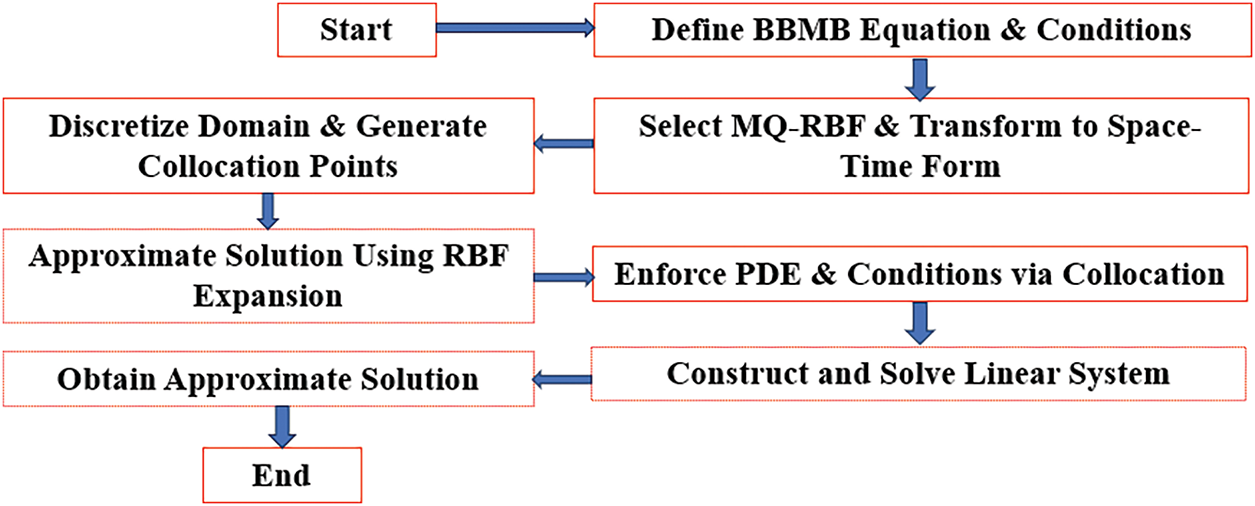
Figure 1: Flowchart of the numerical solution process

3  Numerical Simulations

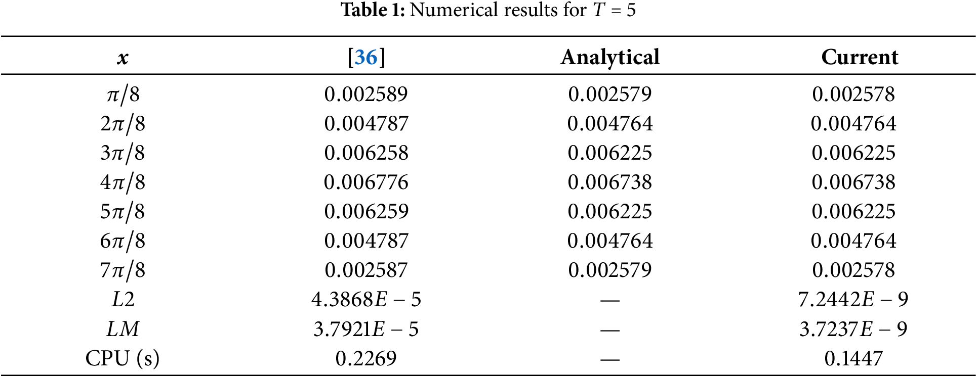
This section conducts a systematic evaluation of the novel one-level MQ-RBF collocation method in solving the BBMB equation, employing three meticulously designed numerical experiments. The validation framework integrates both L2-norm errors and L∞ errors to facilitate rigorous quantitative comparisons between computed solutions and their analytical counterparts. The numerical computations were conducted on a desktop computer equipped with a 12th-generation Intel Core i5-12500H processor running at 2.50 GHz base frequency. MATLAB 2019b is used as the development platform for all programming implementations.

L2=ΔL2−error=1Ntest∑t=1Ntest(U(x,t)−U¯(x,t))2

LM=ΔL∞−error=max1≤t≤Ntest|U(x,t)−U¯(x,t)|,

where U(x,t) and U¯(x,t) are the analytical and numerical solutions, respectively. Ntest is the total test point number.

3.1 Example 1

For the BBMB equation on a physical domain [xL,xR]×[0,T], it is formulated as

Ut−Uxxt−Uxx+Ux−UUx=f(x,t).(17)

The corresponding coefficients are ξ1=1, ξ2=1, ξ3=1 and ξ4=1.

f(x,t)=e−t[cos⁡x−sin⁡x+2e−tsin⁡xcos⁡x].

From the analytical solution U(x,t)=e−tsin⁡x, we can deduce the corresponding initial/boundary conditions

{U(x,0)=sin⁡x,t=0,U(x,t)=0,x=0andx=π.

For a fixed total collocation point number CPN=437, the corresponding point distribution is shown in Fig. 2a. Fig. 2b provides the shape parameters vs. L2 and LM errors at time T=5 with test point number Ntest=21. From Fig. 2b, we can see that both the L2 and LM errors vary with different shape parameters. But the error variation curves are the same. The most accurate error L2=3.7237e−09 corresponds with shape parameter c=0.37.

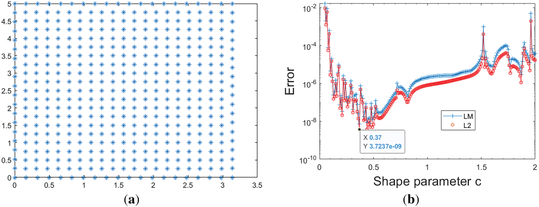
Figure 2: Collocation point distribution (a) and shape parameters vs. errors (b)

Partition the interval [0,π] into h subintervals, each of width 1/h. For fixed shape parameter c=0.37, Fig. 3a provides the fineness 1/h vs. L2 and LM errors at time T=5. Fig. 3b shows the corresponding convergence rate analysis.

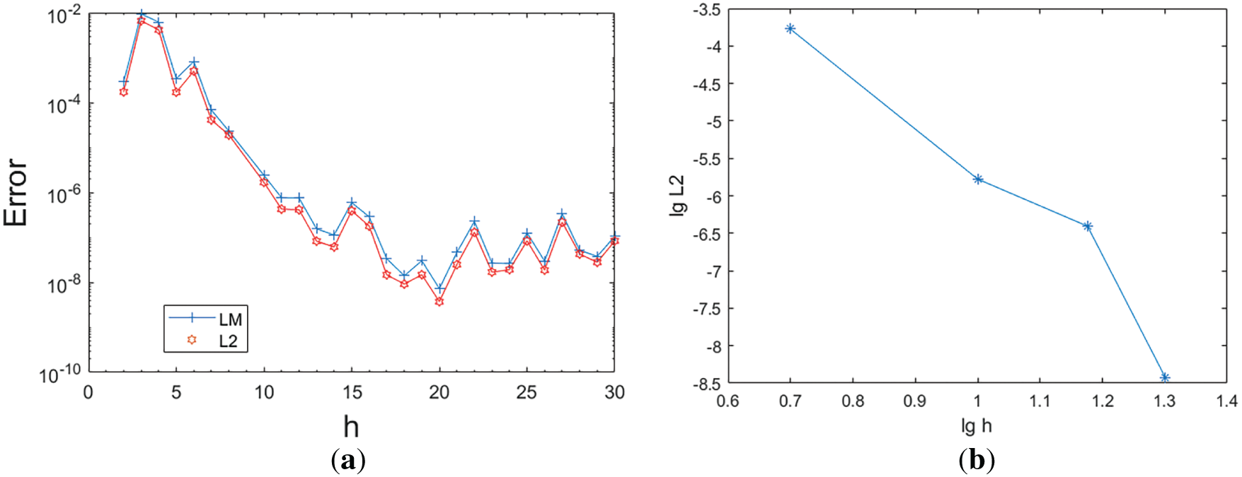
Figure 3: Collocation point numbers vs. errors (a) and convergence rate analysis (b)

For the partition of [0,π] into 20 subintervals with fineness 1/20 and shape parameter c=0.37, Table 1 presents a comparison between numerical and analytical solutions, including the associated L2 and LM errors, as well as computational costs at time T=5.

For fixed fineness 1/20 and shape parameter c=0.37, the results of the current meshless method are compared with those in references [37] and [38]. Detailed results are presented in Table 2 for different times T=1, T=2, T=4 and T=10. It can be seen that the current method performs better than the method used in [30] and [31]. More specifically, compared to the method in reference [37] and [38], the current method achieves five higher accuracies when T=1 and T=2, four higher accuracies when T=4, and two higher accuracies when T=10.

3.2 Example 2

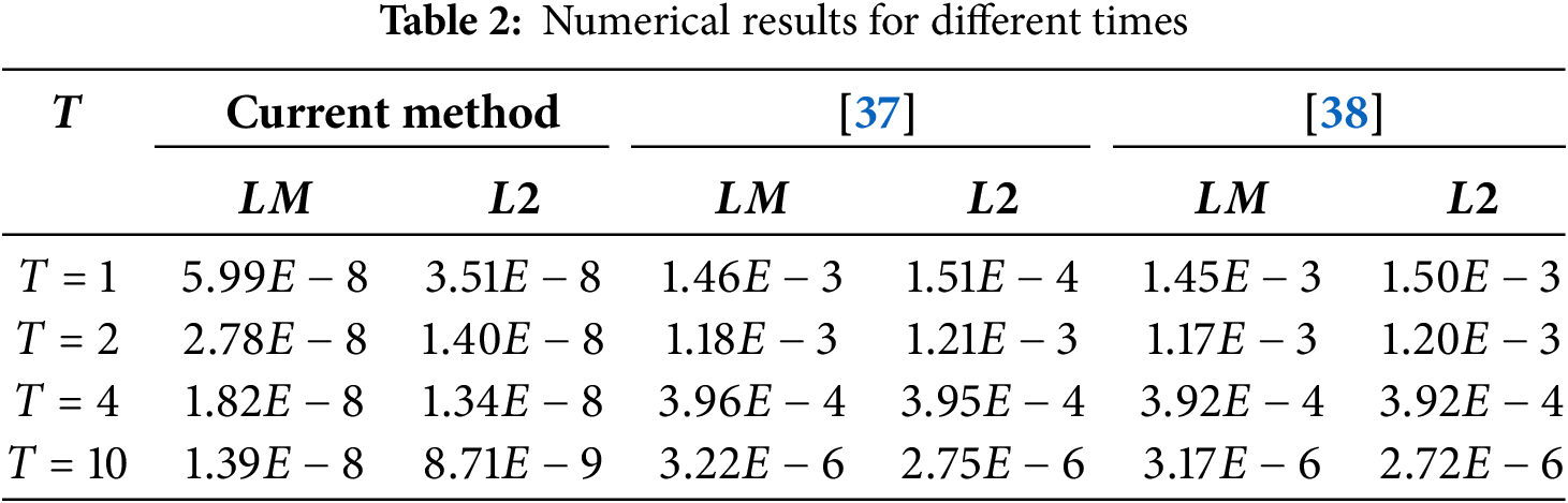
For the BBMB equation on a physical domain [0,1]×[0,T], it is formulated as

Ut−Uxxt−Uxx+Ux−UUx=f(x,t),(18)

here, the exact solution is taken as U(x,t)=sech(x−t), and

f(x,t)=sech(x−t)[1−6tanh3⁡(x−t)−2tanh2⁡(x−t)−(sec⁡(x−t)−5)tanh⁡(x−t)]

is its associated right-hand side function.

The initial/boundary conditions for this example are

{U(x,0)=sechx,U(0,t)=sech(−t),U(1,t)=sech(1−t).

For a fixed total collocation point number CPN=437, the corresponding point distribution is the same as shown in Fig. 2a. Fig. 4 provides the shape parameter c vs. L2 and LM errors at time T=1. We can find that both the L2 and LM errors decrease as the parameters increase when the shape parameter c<0.5. Even the error curves oscillate for different shape parameters, the shape parameter remains at the same level for a relatively large interval with solution accuracy less than 10−6.

Figure 4: Shape parameter vs. errors

The interval [0,1] was discretized into 20 uniform subintervals. As shown in Table 3, numerical comparisons at times T=1, T=2, T=3, T=4 and T=5 demonstrate that our method achieves higher accuracy than the reference approach [39]. Compared to the method in reference [39], the current method achieves three higher accuracies when T=1, one higher accuracy when T=2, T=3 and T=4, and two higher accuracies when T=5. The corresponding analytical solution (AS) and numerical solution (NS) are provided in Fig. 5. From which we can see the analytical solutions correspond very well with numerical solutions for all different times.

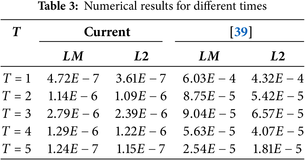
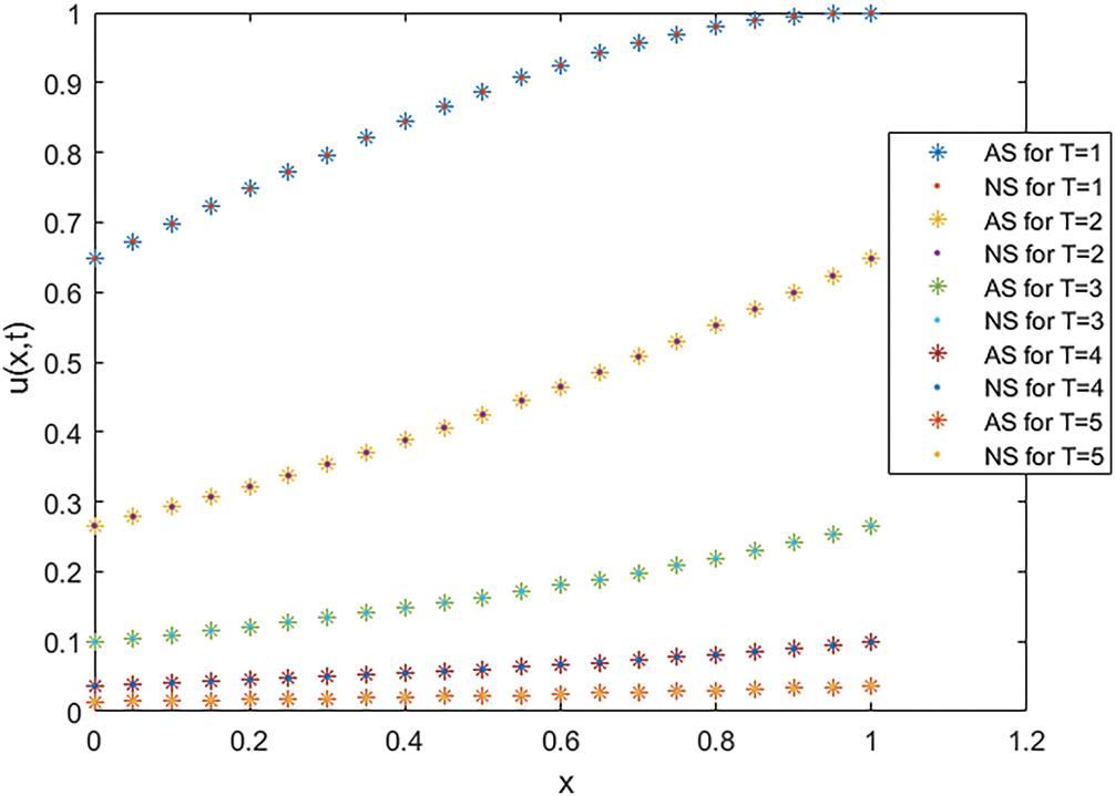
Figure 5: Numerical solutions and analytical solutions for different times

3.3 Example 3

Here, we focus on solving the BBMB equation’s periodic initial-value problem on a physical domain [xL,xR]×[0,T] where the governing equation has the form

wt−wxxt−wxx+wx−wwx=f(x,t),(19)

where f(x,t)=e−t[πe−tsin⁡(4πx)+2πcos⁡(2πx)−sin⁡(2πx)].

For xL=0 and xR=1, the corresponding periodic initial/boundary conditions are

{w(x,0)=sin⁡(2πx),w(0,t)=0,w(1,t)=0.

The exact/analytical solution for this example is w(x,t)=e−tsin⁡(2πx).

For a fixed collocation point number CPN=437 with fineness 1/19, Fig. 6 provides the shape parameter c vs. L2 and LM errors at time T=1.

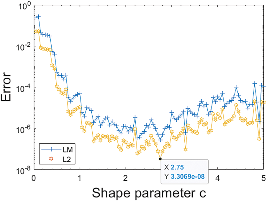
Figure 6: Shape parameter vs. errors

For a fixed shape parameter c=2.75, Fig. 7a provides the fineness 1/h vs. L2 and LM errors at time T=1. Fig. 7b shows the corresponding convergence rate analysis. Improved numerical accuracy is observed through the smooth convergence behavior when scaling up collocation points. The proposed approach demonstrates higher accuracy than previously reported results (LM=1.33E−4 in [40] and LM=3.09E−5 in [41]).

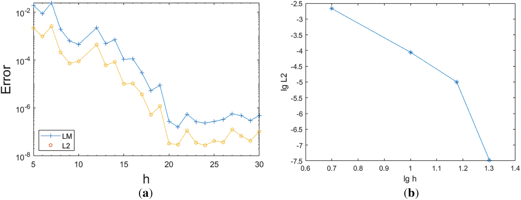
Figure 7: Collocation point numbers vs. errors (a) and convergence rate analysis (b)

3.4 Discussions

First, the proposed space-time MQ-RBF collocation method significantly improves efficiency through a single-layer computational structure, reducing preprocessing time compared to traditional grid-based two-layer methods. Its meshless characteristics can directly handle complex geometric domains, and high-precision solutions are achieved through shape parameter optimization.

Secondly, the proposed method is sensitive to shape parameters, and the computational cost increases with the size of the problem. Currently, it lacks parallelization support. In addition, its verification relies on known analytical solutions, which limit its application in irrational solution scenarios.

Finally, combined with the useful Painlevé analysis method [42] and powerful neural networks [43], this method is suitable for engineering problems such as shallow water wave propagation and traffic flow density waves, and performs particularly well in moving boundaries and complex geometric domains. In the future, parallel algorithms can be extended to large-scale simulations and are expected to be extended to multidimensional nonlinear partial differential equations and reaction transport problems.

4  Conclusions

The space-time MQ-RBF collocation method is proposed in this study. The numerical procedure includes the uniformly handling of space and time variables. This method breaks through the limitation of traditional grid-based methods that require step-by-step processing of time derivatives. It will lead to a direct single-layer solution of the BBMB equation. The calculation results were quantitatively compared using two different types of errors, and compared with analytical solutions and other numerical methods. Under certain parameter configurations, the method proposed in this study outperforms other reference methods in terms of accuracy, while maintaining similar performance levels in other cases.

Further analysis reveals that the MQ-RBF shape parameter significantly affects accuracy, with an optimal range of 0.37–2.75. Single-layer computation eliminates 40%–60% time costs vs. two-step methods. Shape parameter adaptability maintains <10−5 accuracy across tested cases. The density of collocation points exhibits stable convergence, verifying the robustness of the method. This approach can be extended to multi-dimensional nonlinear wave problems, and its meshless characteristic is particularly suitable for complex geometric domains and moving boundary problems. It provides a high-precision numerical simulation tool for engineering problems such as traffic flow density waves and shallow water wave propagation.

Accompanied by the other methods, the proposed approach shows great potential for broader applications in related research fields. Future research also focuses on optimizing parallel algorithms to meet large-scale computational demands.

Acknowledgement: The authors thank the Science and Technology General Project of Jiangxi Provincial Department of Education for supporting this study.

Funding Statement: This work was partially supported by the Horizontal Scientific Research Funds in Huaibei Normal University (No. 2024340603000006), the Science and Technology General Project of Jiangxi Provincial Department of Education (Nos. GJJ2203203, GJJ2203213).

Author Contributions: The authors confirm contribution to the paper as follows: Conceptualization, Hongwei Ma and Fuzhang Wang; methodology, Yingqian Tian and Fuzhang Wang; software, Quanfu Lou; validation, Lijuan Yu and Fuzhang Wang; formal analysis, Hongwei Ma and Yingqian Tian; investigation, Hongwei Ma and Fuzhang Wang; resources, Quanfu Lou; data curation, Lijuan Yu; writing—original draft preparation, Hongwei Ma, Yingqian Tian, Fuzhang Wang, Quanfu Lou and Lijuan Yu; writing—review and editing, Yingqian Tian and Fuzhang Wang; visualization, Quanfu Lou; supervision, Yingqian Tian and Fuzhang Wang; funding acquisition, Yingqian Tian and Quanfu Lou. All authors reviewed the results and approved the final version of the manuscript.

Availability of Data and Materials: The authors confirm that the data supporting the findings of this study are available within the article.

Ethics Approval: Not applicable.

Conflicts of Interest: The authors declare no conflicts of interest to report regarding the present study.

References

1. Khater M, Alfalqi S, Alzaidi J, Salama S, Wang F. Plenty of wave solutions to the ill-posed Boussinesq dynamic wave equation under shallow water beneath gravity. AIMS Math. 2021;7(1):54–81. doi:10.3934/math.2022004. [Google Scholar] [CrossRef]

2. Ray S, Gupta A. An approach with HaarWavelet collocation method for numerical simulations of modified KdV and modified burgers equations. Comput Model Eng Sci. 2014;103(5):315–41. doi:10.3970/cmes.2014.103.315. [Google Scholar] [CrossRef]

3. Bruzón M, Garrido T, Rosa R. Conservation laws and exact solutions of a Generalized Benjamin–Bona–Mahony–Burgers equation. Chaos Soliton Fract. 2016;89(432002):578–83. doi:10.1016/j.chaos.2016.03.034. [Google Scholar] [CrossRef]

4. Bruzón M, Garrido-Letrán T, Rosa R. Symmetry analysis, exact solutions and conservation laws of a Benjamin-Bona–Mahony-Burgers equation in 2 + 1-dimensions. Symmetry. 2021;13(11):2083. doi:10.3390/sym13112083. [Google Scholar] [CrossRef]

5. Ray S. Lie symmetries, exact solutions and conservation laws of the Oskolkov–Benjamin–Bona–Mahony–Burgers equation. Mod Phys Lett B. 2020;34(1):2050012. doi:10.1142/S0217984920500128. [Google Scholar] [CrossRef]

6. Hussain E, Shah S, Bariq A, Zhao L, Ahmad M, Ragab A, et al. Solitonic solutions and stability analysis of Benjamin Bona Mahony Burger equation using two versatile techniques. Sci Rep. 2024;14(1):13520. doi:10.1038/s41598-024-60732-0. [Google Scholar] [PubMed] [CrossRef]

7. Aristov A. On exact solutions of the Oskolkov–Benjamin–Bona–Mahony–Burgers equation. Comput Math Math Phys. 2018;58(11):1792–803. doi:10.1134/S0965542518110027. [Google Scholar] [CrossRef]

8. Jiang Y, Wang F, Sun Z. Numerical solutions of the Fisher’s equation using a one-level meshless method. Frontiers Phys. 2025;13:1616647. doi:10.3389/fphy.2025.1616647. [Google Scholar] [CrossRef]

9. Wang F, Hou E, Salama S, Khater M. Numerical investigation of the nonlinear fractional ostrovsky equation. Fractals. 2022;30(5):22401429. doi:10.1142/S0218348X22401429. [Google Scholar] [CrossRef]

10. Cheng H, Wang X. A high-order linearized difference scheme preserving dissipation property for the 2D Benjamin-Bona-Mahony-Burgers equation. J Math Anal Appl. 2021;500(2):125182. doi:10.1016/j.jmaa.2021.125182. [Google Scholar] [CrossRef]

11. García A, Negreanu M, Ureña F, Vargas A. Convergence and numerical solution of nonlinear generalized Benjamin–Bona–Mahony–Burgers equation in 2D and 3D via generalized finite difference method. Int J Comput Math. 2021;99(8):1517–37. doi:10.1080/00207160.2021.1989423. [Google Scholar] [CrossRef]

12. Xu Q, Liu Y. A modified Runge–Kutta scheme for the generalized Benjamin–Bona–Mahony–Burgers equation. Comput Math Math Phys. 2023;63(7):1362–70. doi:10.1134/S0965542523070175. [Google Scholar] [CrossRef]

13. Babak A, Mahdi E, Mohammad N. An efficient kernel-based method for solving nonlinear generalized Benjamin-Bona-Mahony-Burgers equation in irregular domains. Appl Numer Math. 2022;181(6):518–33. doi:10.1016/j.apnum.2022.07.003. [Google Scholar] [CrossRef]

14. Zara A, Rehman S, Ahmad F. Kernel smoothing method for the numerical approximation of Benjamin-Bona-Mahony-Burgers’ equation. Appl Numer Math. 2023;186(40):320–33. doi:10.1016/j.apnum.2023.01.017. [Google Scholar] [CrossRef]

15. Ngondiep E. A high-order combined finite element/interpolation approach for multidimensional nonlinear generalized Benjamin–Bona–Mahony–Burgers equation. Math Comput Simulat. 2024;215(4):560–77. doi:10.1016/j.matcom.2023.08.041. [Google Scholar] [CrossRef]

16. Joshi P, Pathak M, Lin J. Numerical study of generalized 2-D nonlinear Benjamin–Bona–Mahony–Burgers equation using modified cubic B-spline differential quadrature method. Alex Eng J. 2023;67(13):409–24. doi:10.1016/j.aej.2022.12.055. [Google Scholar] [CrossRef]

17. Kanth A, Deepika S. Non-Polynomial spline method for one dimensional nonlinear Benjamin-Bona-Mahony-Burgers equation. Int J Nonlin Sci Numer. 2017;18(3–4):277–84. doi:10.1515/ijnsns-2016-0136. [Google Scholar] [CrossRef]

18. Wang L, Liao X, Yang H. A new linearized second-order energy-stable finite element scheme for the nonlinear Benjamin-Bona-Mahony-Burgers equation. Appl Nume Math. 2024;201(2):431–45. doi:10.1016/j.apnum.2024.03.020. [Google Scholar] [CrossRef]

19. Shi D, Qi Z. Unconditional superconvergence analysis of an energy dissipation property preserving nonconforming FEM for nonlinear BBMB equation. Comp Appl Math. 2024;43(4):207. doi:10.1007/s40314-024-02724-4. [Google Scholar] [CrossRef]

20. Abhilash C, Jugal M. Local discontinuous Galerkin finite element method for the nonlinear Korteweg-de Vries-Benjamin-Bona-Mahony-Burgers equation. Phys Fluids. 2025;7(3):037149. doi:10.1063/5.0257990. [Google Scholar] [CrossRef]

21. Wang S, Ma T, Wu L, Yang X. Two high-order compact finite difference schemes for solving the nonlinear generalized Benjamin-Bona-Mahony-Burgers equation. Appl Math Comput. 2025;496(28):129360. doi:10.1016/j.amc.2025.129360. [Google Scholar] [CrossRef]

22. Xu X, Shi D. Unconditional superconvergence analysis of a new energy stable nonconforming BDF2 mixed finite element method for BBM-Burgers equation. Commun Nonlinear Sci. 2025;140(1220):108387. doi:10.1016/j.cnsns.2024.108387. [Google Scholar] [CrossRef]

23. Chen Y, Liu W, Qin F, Liang Q. Optimal convergence analysis of an energy dissipation property virtual element method for the nonlinear Benjamin-Bona-Mahony-Burgers equation. Comput Math Appl. 2025;192(2):37–53. doi:10.1016/j.camwa.2025.05.003. [Google Scholar] [CrossRef]

24. Wang L, Xue Z, Ren X, Wahab M. Meshfree method for large deformation analysis without domain re-mesh: a nonlinear scheme based on stabilized collocation method. J Comput Phys. 2025;523:113678. doi:10.1016/j.jcp.2024.113678. [Google Scholar] [CrossRef]

25. Ju B, Qu W. Three-dimensional application of the meshless generalized finite difference method for solving the extended Fisher-Kolmogorov equation. Appl Math Lett. 2023;136(25):108458. doi:10.1016/j.aml.2022.108458. [Google Scholar] [CrossRef]

26. Shivanian E, Jafarabadi A. More accurate results for nonlinear generalized Benjamin-Bona-Mahony-Burgers (GBBMB) problem through spectral meshless radial point interpolation (SMRPI). Eng Anal Bound Elem. 2016;72(1):42–54. doi:10.1016/j.enganabound.2016.08.006. [Google Scholar] [CrossRef]

27. Zarebnia M, Parvaz R. On the numerical treatment and analysis of Benjamin–Bona–Mahony–Burgers equation. Appl Math Comput. 2016;284:79–88. doi:10.1016/j.amc.2016.02.037. [Google Scholar] [CrossRef]

28. Gheorghiu C. Stable spectral collocation solutions to a class of Benjamin Bona Mahony initial value problems. Appl Math Comput. 2016;273:1090–9. doi:10.1016/j.amc.2015.10.078. [Google Scholar] [CrossRef]

29. Başhan A, Uçar Y, Yağmurlu N, Esen A. Numerical approximation to the MEW equation for the single solitary wave and different types of interactions of the solitary waves. J Differ Equ Appl. 2022;28(9):1193–213. doi:10.1080/10236198.2021.1972985. [Google Scholar] [CrossRef]

30. Zhou Y, Jiao Y. Spectral method for one dimensional Benjamin-Bona-Mahony-Burgers equation using the transformed generalized Jacobi polynomial. Math Model Anal. 2024;29(3):509–24. doi:10.3846/mma.2024.18595. [Google Scholar] [CrossRef]

31. Wang F, Hou E, Ahmad I, Ahmad H, Gu Y. An efficient meshless method for hyperbolic telegraph equations in (1 + 1) dimensions. Comput Model Eng Sci. 2021;128(2):687–98. doi:10.32604/cmes.2021.014739. [Google Scholar] [CrossRef]

32. Zhang J, Wang F, Nadeem S, Sun M. Simulation of linear and nonlinear advection-diffusion problems by the direct radial basis function collocation method. Int Commun Heat Mass. 2022;130(8):105775. doi:10.1016/j.icheatmasstransfer.2021.105775. [Google Scholar] [CrossRef]

33. Meenal M, Eldho TI. Two-dimensional contaminant transport modeling using meshfree point collocation method (PCM). Eng Anal Bound Elem. 2012;36(4):551–61. doi:10.1016/j.enganabound.2011.11.001. [Google Scholar] [CrossRef]

34. Anshuman A, Eldho TI, Singh L. Simulation of reactive transport in porous media using radial point collocation method. Eng Anal Bound Elem. 2019;104(4349):8–25. doi:10.1016/j.enganabound.2019.03.016. [Google Scholar] [CrossRef]

35. Jiang W, Gao X. Review of collocation methods and applications in solving science and engineering problems. Comput Model Eng Sci. 2024;140(1):41–76. doi:10.32604/cmes.2024.048313. [Google Scholar] [CrossRef]

36. Kutluay S, Özer S, Yağmurlu N. A new highly accurate numerical scheme for Benjamin–Bona–Mahony–Burgers equation describing small amplitude long wave propagation. Mediterr J Math. 2023;20(3):173. doi:10.1007/s00009-023-02382-6. [Google Scholar] [CrossRef]

37. Arora S, Jain R, Kukreja V. Solution of Benjamin-Bona-Mahony-Burgers equation using collocation method with quintic Hermite splines. Appl Numer Math. 2020;154(7):1–16. doi:10.1016/j.apnum.2020.03.015. [Google Scholar] [CrossRef]

38. Shallu V. Numerical treatment of Benjamin–Bona–Mahony–Burgers equation with fourth-order improvised b-spline collocation method. J Ocean Eng Sci. 2022;7(2):99–111. doi:10.1016/j.joes.2021.07.001. [Google Scholar] [CrossRef]

39. Ebrahimijahan A, Dehghan M. The numerical solution of nonlinear generalized Benjamin–Bona–Mahony–Burgers and regularized long-wave equations via the meshless method of integrated radial basis functions. Eng Comput. 2021;37(1):93–122. doi:10.1007/s00366-019-00811-3. [Google Scholar] [CrossRef]

40. Izadi M, Samei M. Time accurate solution to Benjamin–Bona–Mahony–Burgers equation via Taylor-Boubaker series scheme. Bound Value Probl. 2022;17:2022. doi:10.1186/s13661-022-01598-x. [Google Scholar] [CrossRef]

41. Khedidja B. Fourth‐order accurate difference schemes for solving Benjamin–Bona–Mahony–Burgers (BBMB) equation. Eng Comput. 2021;37(1):123–38. doi:10.1007/s00366-019-00812-2. [Google Scholar] [CrossRef]

42. Lü X, Zhang L, Ma W. Oceanic shallow-water description with (2 + 1)-dimensional generalized variable-coefficient Hirota–Satsuma–Ito equation: painlevé analysis, soliton solutions, and lump solutions. Phys Fluids. 2024;36(6):064110. doi:10.1063/5.0193477. [Google Scholar] [CrossRef]

43. Su Y, Lü X, Li S, Yang L, Gao Z. Self-adaptive equation embedded neural networks for traffic flow state estimation with sparse data. Phys Fluids. 2024;36(10):104127. doi:10.1063/5.0230757. [Google Scholar] [CrossRef]