
 Submit a Paper
 Propose a Special lssue
 Open Access
ARTICLE

Deep Learning-Based Inverse Design: Exploring Latent Space Information for Geometric Structure Optimization
1 Institute of Photonics, Leibniz University Hannover, Welfengarten 1A, Hannover, 30167, Germany
2 Institute for Interdisciplinary Research of Computational Mechanics and Artificial Intelligence, Fudan University, Shanghai, 200437, China
3 Department of Geotechnical Engineering, College of Civil Engineering, Tongji University, Shanghai, 200092, China
* Corresponding Author: Xiaoying Zhuang. Email:
Computer Modeling in Engineering & Sciences 2025, 145(1), 263-303. https://doi.org/10.32604/cmes.2025.067100
Received 25 April 2025; Accepted 06 August 2025; Issue published 30 October 2025
 View Full Text
 Download PDF
Abstract
Traditional inverse neural network (INN) approaches for inverse design typically require auxiliary feedforward networks, leading to increased computational complexity and architectural dependencies. This study introduces a standalone INN methodology that eliminates the need for feedforward networks while maintaining high reconstruction accuracy. The approach integrates Principal Component Analysis (PCA) and Partial Least Squares (PLS) for optimized feature space learning, enabling the standalone INN to effectively capture bidirectional mappings between geometric parameters and mechanical properties. Validation using established numerical datasets demonstrates that the standalone INN architecture achieves reconstruction accuracy equal or better than traditional tandem approaches while completely eliminating the workload and training time required for Feedforward Neural Networks (FNN). These findings contribute to AI methodology development by proving that standalone invertible architectures can achieve comparable performance to complex hybrid systems with significantly improved computational efficiency.Keywords
In the field of material design and optimization, determining the geometry of a material is the crucial first step, serving as the foundation for deciding its mechanical properties and operational performance [1–3]. The geometry of a material can be created using Computer-Aided Design (CAD) tools or through design algorithms based on initial technical requirements [4–6]. Once the geometry is established, mechanical simulations and testing are conducted to evaluate properties such as stiffness, strength, relative density, Poisson’s ratio, and the stress-strain curve [7–9]. The results obtained from this process form the basis for evaluating whether the material meets the design standards. This is a vital process for ensuring that the material can perform effectively in specific applications. However, the traditional design method, known as forward design, while widely used, has some significant limitations [10,11]. This approach is typically linear, beginning with geometric design, followed by simulations and tests to adjust and optimize mechanical properties [12]. This method requires multiple iterations of trial and error, consuming considerable time and computational resources [13]. This makes the design process inefficient, especially when optimizing complex materials with many parameters. To address this issue, inverse design methods based on deep learning have emerged, offering significant improvements. Within inverse design methodology, deep learning models can be used to predict or optimize geometry based on the desired mechanical properties of a material [14–16]. Instead of conducting numerous trials like traditional design, inverse design leverages data from previous experiments to create more accurate and rapid deep learning models [17]. This approach not only reduces the use of trial-and-error iterations but also enhances the efficiency and accuracy of the design process [18]. Through deep learning, models can quickly predict the properties of a material from existing geometry or, conversely, generate new geometries from predefined properties [19].
In material design and optimization, geometric representation plays an essential role in the inverse design process, determining the ability to reproduce and optimize the mechanical properties of a material. Framework for mechanical property prediction and inverse design using neural networks is illustrated, where a parametric geometric model is used to predict or optimize mechanical properties via both forward and inverse neural network approaches, forming an iterative geometry-property refinement loop (see Fig. 1).
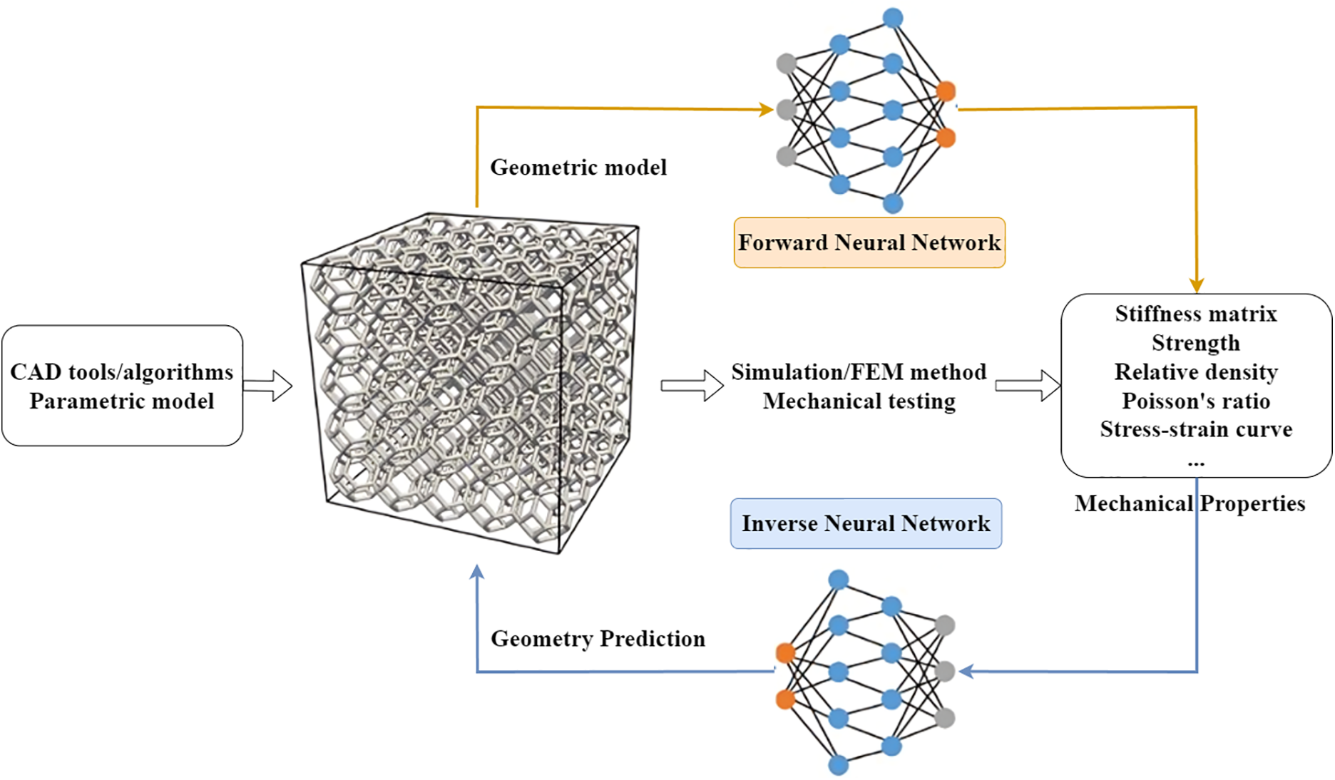
Figure 1: Framework for mechanical property prediction and inverse design using neural networks. A parametric geometric model is generated using CAD tools or algorithms. This geometric model undergoes simulations and mechanical testing to predict mechanical properties like stiffness, strength, relative density, Poisson’s ratio, or the stress-strain curve. A forward neural network (FNN) is employed to predict the mechanical properties based on the geometric model. Simultaneously, an INN is utilized to predict the optimal geometry required to achieve desired mechanical properties, creating a feedback loop for geometry refinement
Common geometric representation methods include voxels, meshes, point clouds, and modeling parameters [20,21]. Each method has its advantages and disadvantages, directly affecting computational costs, file size, model accuracy, and the ability to reconstruct geometry during the inverse design process [20].
• Voxels: This method represents three-dimensional geometry as small elements, similar to pixels in two-dimensional images. Each voxel represents a small volume unit in three-dimensional space, allowing detailed representation of complex geometries at high resolution [22]. While voxels accurately capture the microdetails of materials, the main drawback is the high computational cost and large memory requirement due to the number of voxels needed to describe the detailed geometry [23,24].
• Meshes: Meshes use triangular or quadrilateral grids to simulate the surface of a material and are commonly used in numerical simulations and computer graphics applications [25]. This method is flexible and is capable of accurately simulating the geometry of complex surfaces, especially by reducing the number of elements required compared to voxels, thus reducing computational costs [26]. However, meshes face challenges in simulating internal structures of materials and require complex algorithms to ensure the integrity of the mesh when geometry changes [27,28].
• Point Clouds: Point clouds represent geometry through a set of points in three-dimensional space [29]. This method is often used in 3D scanning and simulating complex geometries such as rough surfaces or materials with discontinuous structures. The strength of point clouds lies in their ability to store detailed geometric information without having to define the topology between points [30]. However, the weakness of this method is the lack of information on how points connect, complicating the reconstruction process and requiring complex algorithms to convert point clouds into usable models in numerical simulations [31,32].
• Modeling Parameters: This approach represents geometry through simple or complex parameters such as size, shape, rotation angles, or other geometric parameters [33,34]. This method focuses on abstracting geometry into a set of parameters, significantly reducing file size and computational costs [35]. However, important geometric details may be lost, if the parameters are not well defined and controlled. This poses a challenge in accurately reconstructing geometry from simplified parameters, especially when simulating complex mechanical properties of materials [8,36,37].
Each geometric representation method offers a different balance between accuracy, computational cost, and geometric reconstruction capability during inverse design. The choice of the appropriate representation method depends on the specific goals of the design and optimization process, as well as the required level of detail and available computational resources.
The essential task of the inverse design starts with the desired mechanical properties of the material, such as stiffness, strength, relative density, and parameters related to stress and strain. Instead of designing the geometry first and then testing the mechanical properties, the inverse design takes the opposite approach: using the desired mechanical properties to predict and optimize the geometry of the material [38–40]. Advanced deep learning models or optimization algorithms are applied to find the optimal geometry, minimizing dependence on traditional physical experiments, which are often complex and costly. This brings breakthroughs in material design, allowing the creation of materials with mechanical properties precisely tailored to the requirements [41–44]. There are three common types of inverse design, each using different approaches to achieve optimization goals:
• Indirect Inverse Design: This method begins by using deep learning models to predict mechanical properties based on existing geometry. Subsequently, optimization algorithms, such as metaheuristic algorithms (e.g., evolutionary strategies, genetic algorithms), search for the optimal geometry that satisfies the mechanical property requirements [45,46]. The indirect inverse design is flexible for a wide range of models and is often used when there is no direct and clear relationship between geometry and mechanical properties. However, the drawback of this method is the high computational cost, as it requires optimizing a cost function over a broad search space with numerous parameters [47–49].
• Direct Inverse Design: In this approach, deep learning models are used to directly generate or optimize geometry based on predefined mechanical properties without an intermediary step [16]. This is a one-way process where the mechanical properties are used as input and the deep learning model instantly creates the corresponding geometry [50,51]. Direct inverse design is highly effective in generating materials with complex geometries, as it avoids trial-and-error steps during optimization. However, this method requires a large amount of data to train the deep learning model and may struggle with handling broad search spaces with a large number of parameters [52–54].
• Semi-Direct Inverse Design: This method combines the strengths of both indirect and direct inverse design. Initially, it uses modeling parameters to narrow the search space, simplifying, and making the optimization process more efficient. The results are then refined using deep learning models to achieve optimal geometry. Semi-direct inverse design reduces computational costs by limiting the search range while still leveraging deep learning’s power for precise geometric optimization. This allows a balance between accuracy and computational efficiency, which is particularly useful when working with materials that have complex structures [55,56].
Each inverse design method has its advantages and limitations, and selecting the appropriate method depends on material properties, technical requirements, and available computational capabilities. In the future, the flexible combination of these methods, along with the advancement of deep learning and optimization algorithms, will continue to open new opportunities in the design and production of advanced materials.
Inverse design not only helps optimize the material design process, but also opens up new opportunities for creating materials with superior mechanical properties that meet stringent technical requirements. With the rapid development of deep learning and artificial intelligence, this field promises significant advances in designing and manufacturing high-tech materials.
This research will continue to develop the inverse design method with novel ideas:
Architectural Innovation: Standalone INN như paradigm shift trong neural network design
• Computational Efficiency: Elimination of FNN as sustainability contribution
• Methodological Advancement: Gaussian integration into INN as novel regularization approach
• Scalability Potential: Framework applicability across diverse materials domains, validated on 2 different types of materials and experiments in 2 independent datasets.
2.1 Geometric Representation in Inverse Design
A central aspect of inverse design in material science is the choice of geometric representation. These different geometric representation methods are illustrated in Fig. 2, showing how the same structural geometry can be visualized using meshes, voxels, and point clouds. Each method offers distinct trade-offs in terms of geometric detail, data size, computational cost, and compatibility with deep learning models.
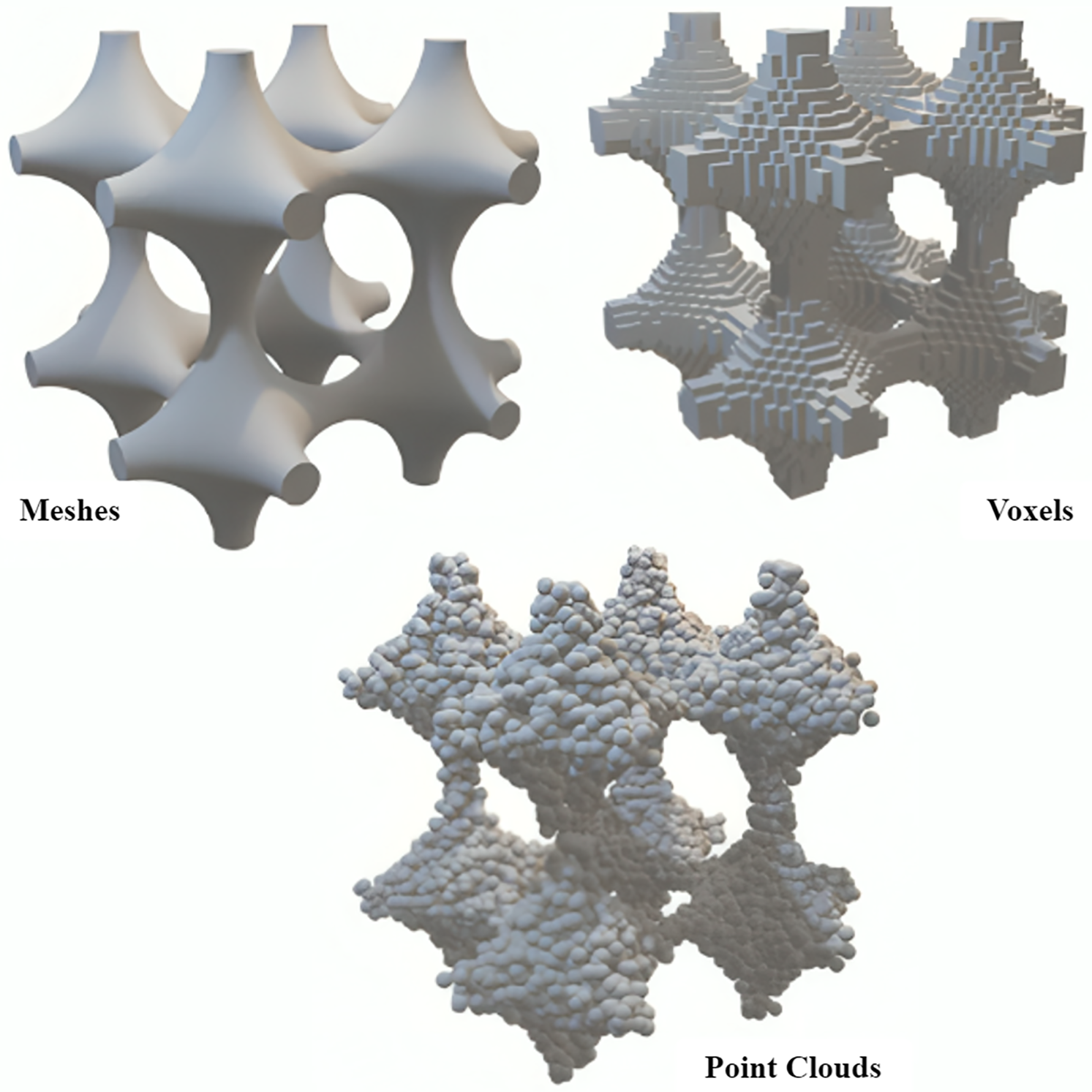
Figure 2: Geometric representations of the model based on different parameterization approaches. The modeling parameters enable representation of the same geometric structure in different spatial formats, including voxels, meshes, and point clouds. These representations provide different ways to visualize and analyze the structure for various computational or simulation purposes, with each format having specific applications in computational mechanics, rendering, or data analysis
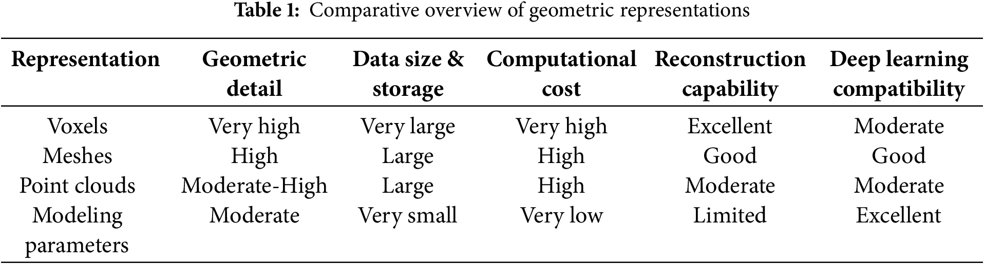
Modeling parameters abstract geometry into a set of key variables (e.g., size, shape, orientation), dramatically reducing data size and computational requirements compared to voxel, mesh, or point cloud representations. This makes them highly suitable for deep learning-based optimization and rapid algorithmic validation, especially when working with large datasets or limited computational resources (see Table 1 for a detailed comparison of geometric representation methods).
In this study, modeling parameters are used as the geometric representation for three main reasons:
• Efficiency: They enable a significant reduction in both file size and computational cost, crucial for iterative model development and benchmarking.
• Dataset Alignment: The benchmark datasets used (Kumar et al., 2020 [57]; Ha et al., 2023 [58]) are already parameterized, allowing for direct comparison and validation of algorithmic advances.
• Focus on Algorithmic Effectiveness: The primary aim is to validate the core semi-direct inverse design framework, rather than to target a specific geometric structure or application.
As shown in Fig. 3, modeling parameters were chosen for their unique balance of efficiency, scalability, and compatibility with deep learning. Although this work does not directly target voxel, mesh, or point cloud data, the framework is theoretically extensible to those formats by mapping them into a lower-dimensional latent or parameterized space.
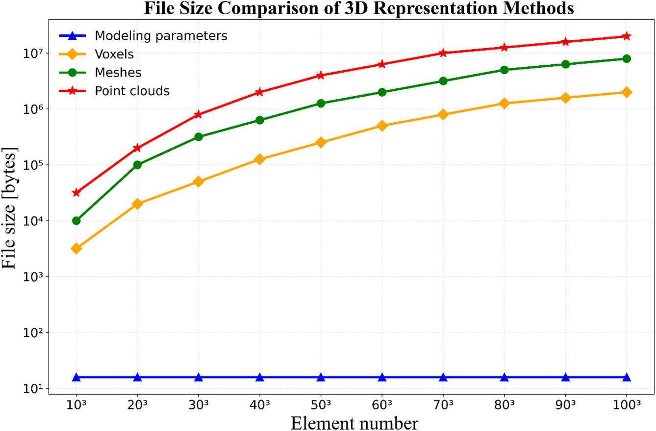
Figure 3: File size comparison of different geometric representations as a function of the number of elements. The plot shows how file size (in bytes) scales with increasing element numbers for different geometric representations
2.2 Detailed Benchmark Datasets and Rationale for Data Preparation
The present study selects and prepares two public datasets, each designed to present a strict one-to-one mapping suitable for rigorous evaluation, interpretable dimensionality reduction, and trustworthy model validation. The following outlines the motivation, structure, preprocessing strategies, and justifications for the curation and use of these datasets, as well as the logic guiding their incorporation within the proposed standalone INN methodology.
2.2.1 Motivation and Principles for Dataset Selection
A fundamental goal of inverse design is to reconstruct optimal geometric configurations that yield tailored mechanical responses. Achieving this necessitates datasets that (i) encode explicit, reproducible relationships between geometric parameters and target properties, and (ii) include sufficient diversity and statistical regularity for model training. The two selected datasets—derived respectively from Kumar et al. [57] and Ha et al. [58]—fulfill these criteria based on the following principles:
• Transparent Parametrization: Both datasets parameterize geometry via well-defined, low-dimensional feature sets. This facilitates clear attribution of mechanical outcomes to their geometric origin and supports subsequent feature engineering without loss of interpretability.
• One-to-One Mapping: Duplicate and highly ambiguous mappings are removed to ensure that each geometry uniquely corresponds to a set of mechanical properties, and vice versa. This sharpens model learning and validation.
• Suitability for Latent Space Methods: The inherent structure and statistical properties of both datasets allow for efficient application of principal component analysis (PCA) or partial least squares (PLS), enabling effective dimensionality reduction and information condensation.
2.2.2 Structure and Preparation of Individual Datasets
Kumar et al., 2020 [57] Dataset: Spinodoid Metamaterials
This dataset focuses on a new class of spinodoid metamaterials defined by non-periodic topologies inspired by spinodal decomposition. Each entry consists of four continuous geometric parameters: relative solid volume fraction (volFrac) and three principal orientation angles (thetaX, thetaY, thetaZ), together describing the anisotropic architecture. Mechanical properties are encoded as a nine-dimensional stiffness tensor, providing a complete record of the elastic response. Systematic preprocessing is employed:
• Outlier Removal: A robust z-score criterion is used to exclude samples exhibiting extreme property distributions, addressing potential gradient instability during training.
• Duplicate Elimination: Repeated samples are identified and removed to maintain data integrity and avoid skewing validation metrics.
• Standardization: All continuous features are z-score normalized, ensuring consistent scaling and unbiased optimization during subsequent model training.
• Dimensional Reduction: Owing to the strong linear relationship present in the dataset, PCA is employed.
Ha et al., 2023 [58] Dataset: Architected Elastomer Lattices
The Ha et al. dataset is built on high-fidelity experimental measurements of architected elastomer lattices, encoding both geometric and mechanical diversity relevant to practical materials engineering. Its design emphasizes the capacity to reproduce a wide range of stress–strain curve behaviors. Dataset characteristics include:
• Geometric Parameters: Seven variables combining one continuous ratio, one angular parameter, and five categorical descriptors (expressed as one-hot vectors), reflecting both shape and topology.
• Mechanical Properties: Thirteen descriptors derived from stress–strain measurements, systematically covering linear limits, extrema, and terminal states.
• Expansion and Cleansing: The initial set of 280 samples is expanded to 2808 through guided feature engineering, ensuring richer coverage of the design space.
• Latent Feature Extraction: Given the dataset’s pronounced nonlinear and mixed-type relationships, PLS regression is used to maximize geometry–property covariance.
The subsequent Section 2.3 will address the challenges arising from using datasets where the material geometry is described in the form of modeling parameters. This geometric representation abstracts the structure into parameterized variables instead of detailed geometric descriptions. Although this abstraction reduces data dimensionality and computational costs, it inevitably leads to a loss of important information linking geometry and mechanical properties. This loss makes it difficult to accurately predict or reconstruct geometry from mechanical data, especially when complex nonlinear interactions or excessive information compression are involved.
To overcome these limitations, the proposed solution employs dimensionality reduction techniques such as Principal Component Analysis (PCA) and Partial Least Squares (PLS). Applying PCA/PLS creates a latent space wherein the most significant information correlating mechanical properties and geometric parameters is recovered and emphasized relative to the original space. The principal components or latent variables are selected to maximize the covariance between the two domains, thereby restoring a close one-to-one mapping ideal between geometry and material properties.
A standalone inverse neural network (INN) is developed to reconstruct the inverse mapping from mechanical properties back to modeling parameters independently, without relying on a feedforward neural network (FNN) for guidance. This framework is particularly suited and experimentally validated on datasets such as Kumar et al. [57] and Ha et al. [58] which exemplify typical one-to-one mappings between parameterized geometry and mechanical properties.
2.3 Challenges and Solutions in Using Modeling Parameters
Challenges:
Loss of Geometric Detail: When representing complex material structures using a set of modeling parameters (such as size, orientation, or volume fraction), a significant amount of fine-scale geometric information is inevitably lost. Unlike voxel or mesh representations, which can capture intricate microstructural features in three-dimensional space, modeling parameters abstract the geometry into a lower-dimensional space. This abstraction is efficient for computation and storage, but it can obscure subtle geometric characteristics that may have a critical impact on mechanical properties. As a result, the direct relationship between geometry and properties becomes less explicit, making it more challenging to accurately predict or optimize material performance, especially for designs where microstructural nuances are essential.
Difficulty in Geometry Reconstruction: Another major challenge arises when attempting to reconstruct the original or target geometry from a limited set of parameters. Deep learning models trained on parameterized data may struggle to generate geometries that faithfully represent the intended structure, particularly when the mapping from properties to parameters is highly nonlinear or underdetermined. This can lead to designs that, while computationally efficient, may not meet the required fidelity in real-world applications. Furthermore, the lack of detailed geometric information increases the risk of generating physically invalid or non-manufacturable structures, which undermines the reliability of the inverse design framework.
Proposed Solutions
Dimensionality Reduction and Feature Engineering: to mitigate the loss of geometric detail, the methodology incorporates dimensionality reduction techniques such as Principal Component Analysis (PCA) and Partial Least Squares (PLS). By transforming the original set of mechanical property data into a condensed set of principal components or latent features, these methods capture the most informative and correlated aspects of the data. The resulting features are then used to supplement the original modeling parameters, effectively restoring some of the lost connections between geometry and mechanical properties. This approach enables the deep learning model to learn more nuanced relationships and improves its ability to generalize across different design scenarios. For example, in the present study, using the top principal components as additional inputs significantly enhanced the accuracy of geometry reconstruction and property prediction.
Standalone Inverse Neural Network (INN): the core of the proposed solution is the development of a standalone INN that is trained using both the original mechanical properties and the transformed features from PCA or PLS. Unlike traditional frameworks that require continuous feedback from a Forward Neural Network (FNN) during training, the standalone INN is designed to independently learn the complex, often indirect, mapping from desired properties to modeling parameters. This independence simplifies the training process, reduces computational costs, and allows the INN to focus on optimizing the inverse mapping. Empirical results show that the standalone INN can achieve high reconstruction accuracy (R2 > 99% in benchmark datasets), even when working with condensed or abstracted input data. The use of advanced loss functions and regularization techniques further enhances the model’s robustness and ability to avoid overfitting.
Validation via Forward Neural Network (FNN): to ensure that the geometries generated by the inverse design process are not only mathematically valid but also meet the prescribed mechanical property requirements, a pre-trained Forward Neural Network (FNN) is employed for validation. After the INN generates a set of modeling parameters, these are passed through the FNN to predict the resulting mechanical properties. The predicted properties are then compared to the original design targets, closing the loop between geometry and function. If the generated geometry fails to meet the target properties, the INN can be retrained or further optimized. This validation step is crucial for maintaining the reliability and practical utility of the inverse design framework, especially when applied to real-world material systems where performance requirements are stringent.
Generative Capability and Diversity Enhancement: to further address the challenge of generating diverse and manufacturable geometries from limited parameters, the methodology introduces controlled randomness into the INN, for example, by adding Gaussian noise during training. This allows the model to produce multiple plausible geometric solutions for a given set of mechanical properties, mimicking the generative behavior of models like Variational Autoencoders (VAE) or Generative Adversarial Networks (GAN), but without relying on complex adversarial training or additional network components. The level of randomness is carefully tuned to balance diversity and accuracy, ensuring that all generated geometries remain within acceptable property ranges.
For more specific information, please refer to the Appendix, which provides detailed supplementary content to ensure transparency, reproducibility, and rigorous evaluation of the study.
3.1 Neural Networks in Inverse Design
FNN serve as crucial control mechanisms in inverse design processes, working in conjunction with INN. The primary role of FNN is to ensure that geometries generated by INN meet both structural and mechanical requirements [58,59]. This approach has proven effective in optimizing geometric reconstruction while maintaining desired mechanical characteristics [13,60].
The advantages of FNN-INN mechanism is the effective handling of one-to-one relationships in metamaterials, particularly for anisotropic materials. While, its limitations is the heavy reliance on FNN accuracy for both measurement and control during INN training.
3.2 Geometry-Mechanical Property Relationships
The relationship between geometry and mechanical properties follows different paradigms in theoretical and practical applications:
FEM Simulation: Provides accurate calculations of mechanical properties through detailed computational mesh and material modeling [61,62]. In ideal conditions, each unique geometric structure corresponds to a specific set of mechanical properties [63].
Real-World Applications: Measurement limitations and environmental factors often lead to many-to-one relationships, where different geometries may yield similar mechanical properties within measurement error margins [64].
3.3 Theoretical Framework of INN-FNN Relationship
The FNN functions as a “surrogate model” system in the inverse design process, providing a mapping function from geometry space to mechanical properties space. When the INN generates geometry, this output is evaluated through the FNN to predict corresponding mechanical properties [65]. This FNN-INN model is also known as Tandem Neural Network, combining INN and FNN into a hybrid system, where FNN provides feedback to optimize INN. This system’s effectiveness relies on the premise that accurate geometric input to FNN yields precise mechanical property predictions.
Research indicates that higher INN accuracy correlates with improved overall system performance [66,67]. When INN generates geometries with high precision, these outputs closely align with the FNN’s training space, leading to enhanced structural correctness, preserved spatial characteristic, improved mechanical property predictions [68–70].
The relationship between INN and FNN is underpinned by several key theoretical principles:
• Direct Mapping Optimization: Single-step optimization from input to output proves more efficient than multi-step processes.
• Expected Risk Minimization: Direct INN optimization reduces the need for secondary evaluation steps.
• One-to-One Mapping: In cases of direct geometry-to-property relationships, FNN re-evaluation becomes redundant.
The implementation of an independent INN approach offers significant advantages. They are, resource optimization by eliminating the need for secondary model training, reduced computational complexity due to lack of adjustment steps from FNN, performance enhancement by focused development of INN capabilities and self-optimization for property maintenance.
The independent INN strategy is validated by evaluation of published INN research featuring FNN involvement, construction of standalone INN without FNN guidance or by employment of FNN as a validation tool for geometric outputs.
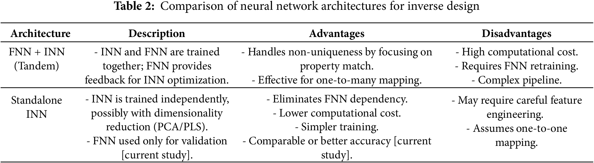
Our methodology aims to demonstrate that in one-to-one relationships between geometry and mechanical properties, an optimized INN can independently achieve required design objectives without continuous FNN oversight. The conceptual differences between traditional Tandem Neural Network and the proposed independent INN strategy are illustrated in Fig. 4 and summarized in Table 2. As shown, Fig. 4a depicts the conventional approach where INN and FNN are coupled for iterative optimization and validation, while Fig. 4b demonstrates the standalone INN implementation with a direct one-to-one mapping between modeling parameters and mechanical properties.
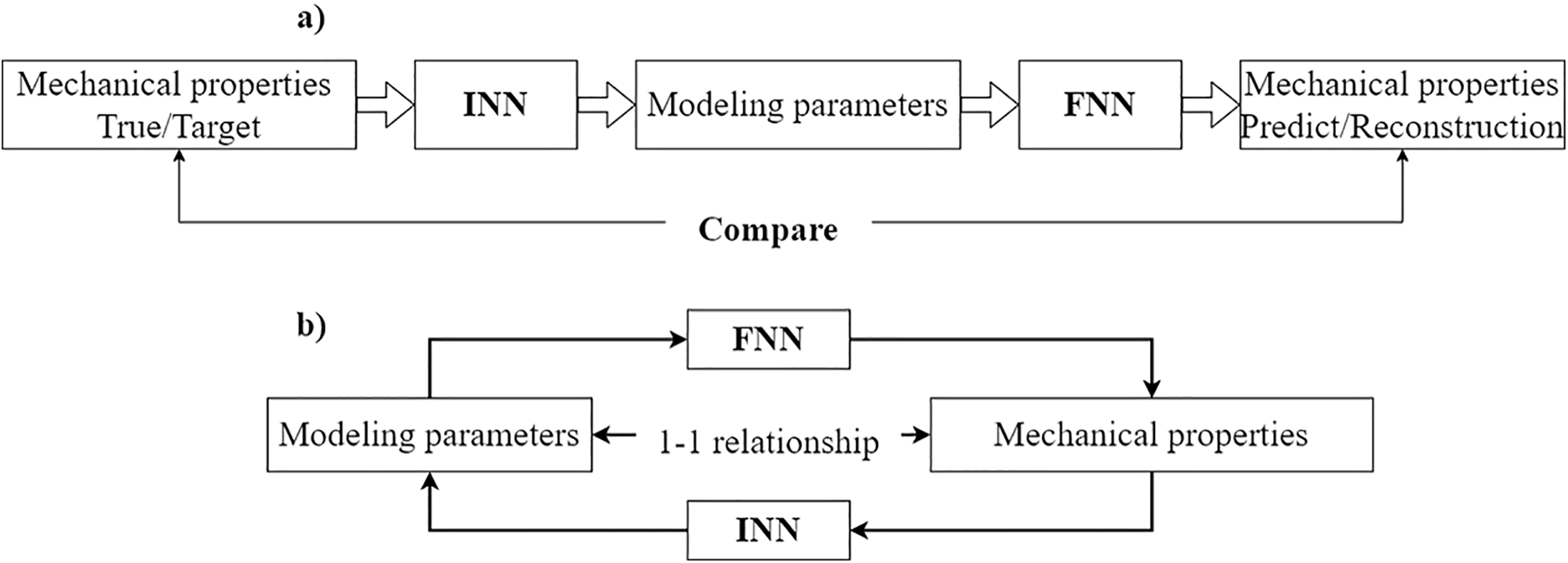
Figure 4: Comparison of two frameworks for mechanical property prediction using FNN and INN. (a) Reconstruction framework: In this approach, the true mechanical properties are provided to the INN to generate the corresponding modeling parameters. These parameters are then passed to the FNN to predict the mechanical properties. The predicted properties are compared to the true properties, creating a feedback loop for reconstruction. This iterative process continues until the predicted properties closely match the true properties, ensuring accurate modeling. (b) Simplified 1-to-1 relationship framework: If there exists a 1-to-1 relationship between the modeling parameters and the mechanical properties, the framework is simplified. The INN can be built directly and independently of the FNN. In this case, INN can map mechanical properties directly back to modeling parameters without relying on FNN, since each set of modeling parameters corresponds uniquely to one set of mechanical properties. This removes the need for iterative feedback between the two networks, making the design process more straightforward
3.4 Dimensionality Reduction for Enhanced Inverse Mapping
When using modeling parameters to represent geometry, essential information linking geometry to mechanical properties is often lost due to the abstraction and compression of data, the reason for the necessity of FNN in Tandem Neural Network. So to remove the influence of FNN, we need a way to restore and enhance the connection between mechanical properties and modeling parameters by using data-dimensional transformation methods. This approach helps create an indirect space, supplementing the information necessary to increase the accuracy of reconstructing modeling parameters. As mentioned above, using modeling parameters to describe a geometry inherently results in the loss of direct information from the geometric model to the mechanical properties. Therefore, if an indirect space can be constructed where the mechanical properties are represented in a different form that strongly links to the modeling parameters, it can help recover some of the lost information.
There are many dimensional transformation methods, including basic and easy-to-implement ones like PCA (Principal Component Analysis) and PLS (Partial Least Squares), which represent data with fewer, more condensed dimensions. This study conducts two evaluations using these methods to evaluate their effectiveness.
Feature Extraction via PCA/PLS
Apply PCA or PLS to the mechanical property dataset, projecting it into a lower-dimensional space where the principal components (or latent variables) capture the most significant variance or correlation with the outputs. These new features act as supplementary links, providing the INN with additional, highly-informative cues for mapping back to modeling parameters.
3.4.1 Principal Component Analysis (PCA)
Objective: Transform original mechanical properties into a lower-dimensional latent space while preserving maximum variance.
Input: Matrix
Mathematical Steps:
1. Standardize
2. Compute covariance matrix:
3. Eigendecomposition:
4.
Project data into latent space:
•
• Latent matrix
Mathematical outcome:
where
Modeling parameters lose geometric details, but PCA extracts latent features maximizing variance in mechanical properties. These features implicitly encode geometric information via correlations (e.g., PC1 strongly correlates with volume fraction (y_col1) in Study Model 1).
Dataset for this case: Kumar et al., 2020 [57]. The characteristics of this dataset make PCA a suitable choice for this case study:
• Large size, clear one-to-one relationship between geometric parameters (volFrac, thetaX, thetaY, thetaZ) and mechanical properties (9 stiffness components).
• Data exhibits strong linearity with minimal noise.
3.4.2 Partial Least Squares (PLS)
Objective: Maximize covariance between mechanical properties (
Input:
Mathematical Steps:
1. Weight vectors: For each latent component h
solved via singular value decomposition (SVD) of
2. Latent scores:
3. Deflate matrices:
4. Latent matrix:
5. Mathematical outcome (similar to PCA):
where
PLS explicitly maximizes Cov(X, Y), directly linking mechanical properties to geometric parameters. In Study Model 2, PLS components (e.g., PLS1–PLS8) showed strong correlations with outputs, enabling accurate INN predictions.
Dataset for this case: Ha et al., 2023 [58]. The characteristics of this dataset make PLS a suitable choice for this case study:
• Small dataset: 280 raw samples, expanded to 2808 through feature engineering.
• Complex nonlinear relationship: Between 13 mechanical properties and 7 geometric parameters (including categorical variables).
• Diverse outputs:
• 5 categorical variables (one-hot encoded).
• 1 binary variable.
• 1 continuous variable.
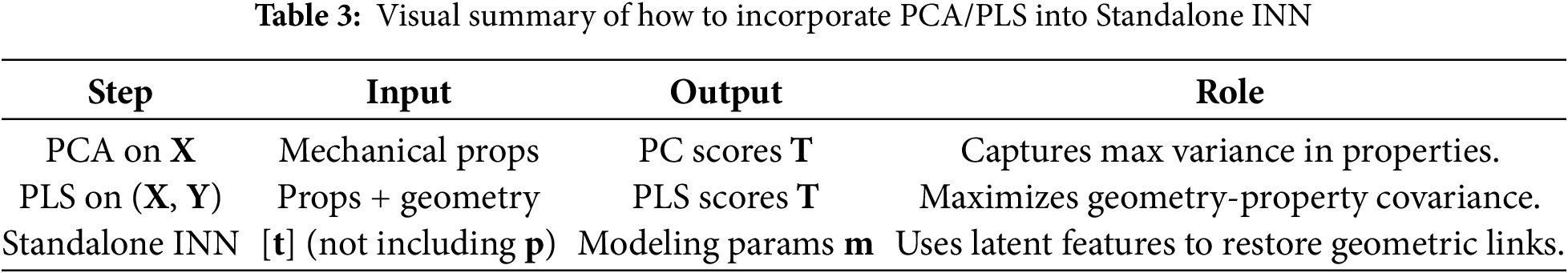
The combined input (p, t) compensates for abstraction losses, achieving near-perfect reconstruction, visual summary as shown in Table 3:
3.5 Mathematical Formulation of Inverse Design with Latent Space
Base on the dimensionality reduction strategies outlined in Section 3.4, by projecting high-dimensional property data into a well-structured latent space using PCA or PLS, the subsequent task is to architect an inverse neural network (INN) that robustly maps condensed property descriptors back to the original or optimal modeling parameters.
To formalize the process, let
The core objective becomes learning a function
where each layer
The training aim is to minimize the mean squared error (MSE) between the predicted geometric parameter vector m^im^i and the ground-truth mimi over all training samples:
optionally augmented by a regularization term
During training, the loss function is minimized using stochastic gradient-based optimizers such as Adam, with key hyperparameters (learning rate, batch size, early stopping patience) set to ensure generalization and reproducibility. All latent variables are standardized, and data splits are stratified to achieve broad coverage of the design space.
By explicitly leveraging the latent spaces constructed in Section 3.4, the approach ensures that only the most informative and robust correlations are utilized, improving both the accuracy and interpretability of the inverse design process. The next section will detail empirical verifications and performance analyses carried out with this formulation.
The research data in this study are sourced from two publications: Kumar et al., 2020 [57] and Ha et al., 2023 [58]. Both data sets used in this investigation exhibit a one-to-one relationship between mechanical properties and geometry in the form of modeling parameters. In other words, there are no two data points in the entire dataset that share the same mechanical property or modeling parameter.
In Kumar’s study, the data is divided into two main categories: modeling parameters and mechanical properties. Modeling parameters include four variables: volume fraction (volFrac), X-axis angle (thetaX), Y-axis angle (thetaY), and Z-axis angle (thetaZ). Mechanical properties are represented by nine components of the stiffness matrix, reflecting the mechanical characteristics. To perform the calculations, a FNN is pre-trained to approximate the FEM and predict mechanical properties from the modeling parameters. In this process, the configuration of the FNN is maintained as presented in Kumar’s publication to ensure consistency and direct comparability with previous results. The FNN is used as a measurement tool to evaluate the ability to accurately reconstruct or predict mechanical properties based on the input modeling parameters, as shown in Fig. 5. The INN network that involves the FNN is called INN-Guide. The R2 score between the mechanical properties generated by the INN (measured by the FNN) and the desired mechanical properties reaches up to 99.9%.
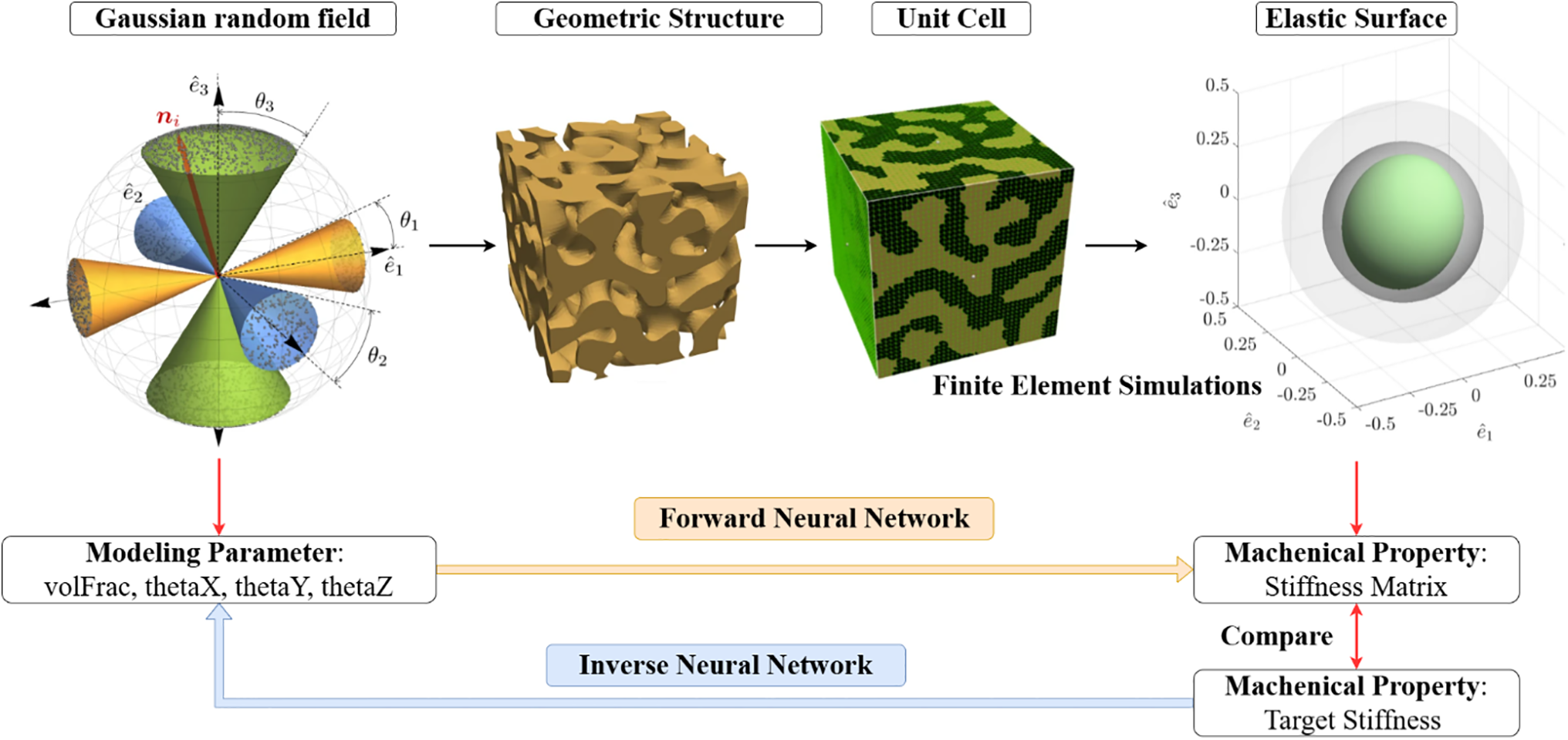
Figure 5: Kumar et al.’s method of parameterizing geometric data and applying it to the inverse design problem [57]
Currently, the goal is to develop a new “independent” INN that achieves higher accuracy than the INN-Guide without the need for FNN support during training, using information from an indirect-dimensional space. To achieve this goal, the data need to be transformed into a different space using techniques such as PCA, as shown in Fig. 6. The features in this new space are condensed and have a clear correlation with the output. Analyzing the correlation between these new features and the output components of the “independent INN” will help determine the number of features that will be used as input for the INN network. Typically, the number of features in the new space will be fewer than in the original space, optimizing the learning process of the independent INN and enhancing the model’s generalization ability.
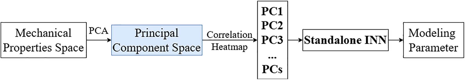
Figure 6: Framework for using Principal Component Analysis (PCA) with a standalone inverse neural network (INN) for predicting modeling parameters from mechanical properties. The process begins by applying PCA to the mechanical properties space to reduce dimensionality and project the properties into a principal component (PC) space. A correlation heatmap is then generated to analyze the relationships between the principal components (PC1, PC2, PC3, etc.). These principal components are subsequently fed into a standalone INN, which predicts the corresponding modeling parameters. This method leverages PCA to simplify the data representation, making it easier for the INN to map mechanical properties to the modeling parameters
In the PCA method, the new space created has a number of dimensions less than or equal to the original space. After applying PCA, analyze the influence of the nine new features in this space on the output of the INN and obtain a heatmap. From this heatmap, it is observed that the last two features, PC8 and PC9, have almost no strong correlation with the output of the INN, as shown in Fig. 7. Therefore, decided to select seven features (PC1 to PC7) as input for the “independent INN” instead of using all nine features from the stiffness matrix, as in the INN-Guide.
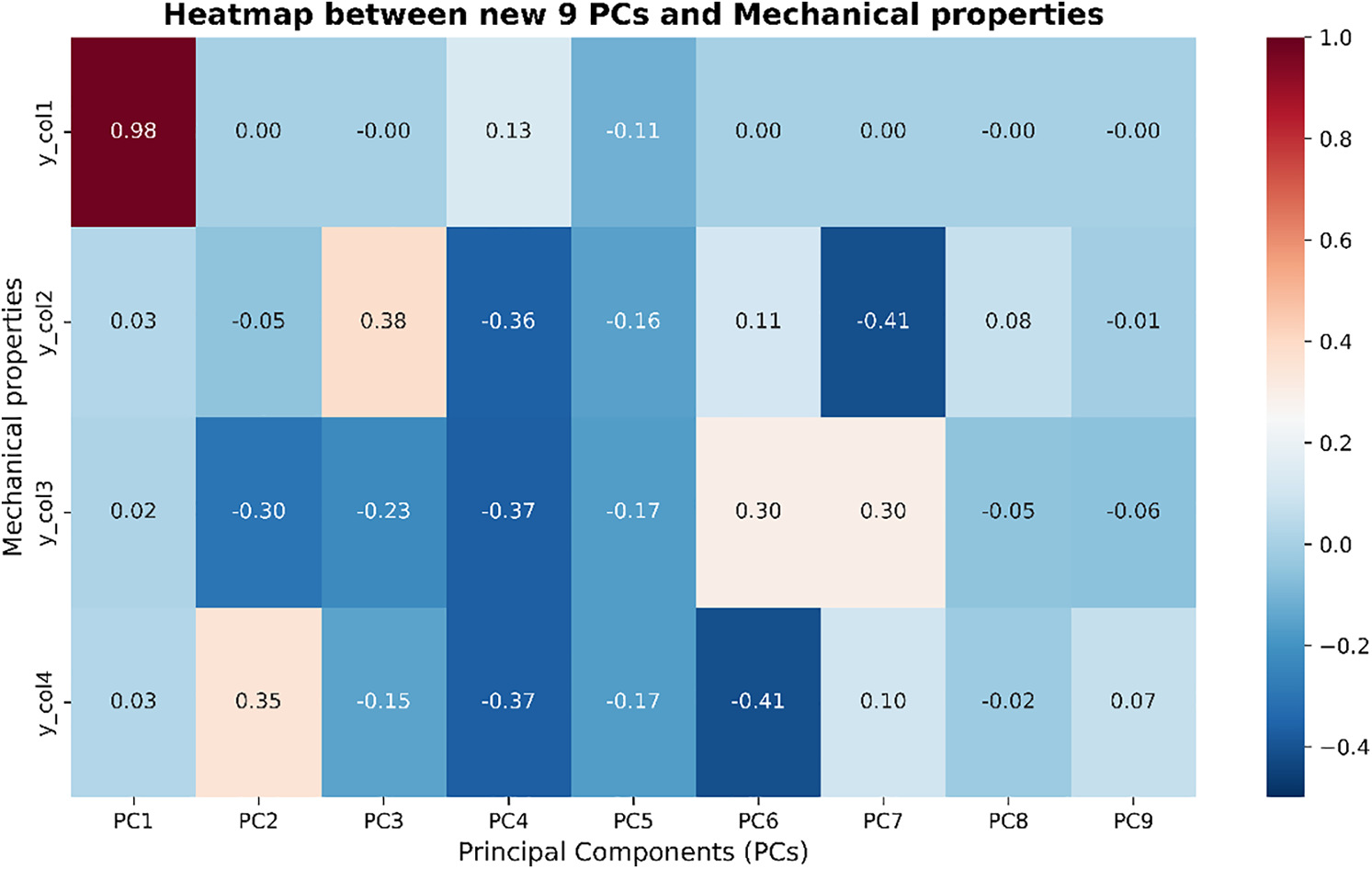
Figure 7: Correlation heatmap between the first 9 principal components (PCs) and selected mechanical property columns. This heatmap visualizes the correlation values between 9 principal components (PC1–PC9) and mechanical properties (y_col1, y_col2, y_col3, and y_col4). The darker shades indicate stronger correlations. From the heatmap, PC1 shows a very high correlation (0.98) with y_col1, while other PCs (especially PC3 and PC4) show moderate correlations with y_col2, y_col3, and y_col4. Based on this analysis, principal components PC1 through PC7 are selected for further modeling as they exhibit notable correlations, whereas PC8 and PC9 are excluded due to their negligible contributions
Among the seven selected components, PC1 has a strong influence on the first output component, namely volFrac. This suggests that the “independent INN” will achieve high accuracy for the volFrac component. The R2 score results for the “independent INN” when using seven PCs from the new space are 99.71%, 83.41%, 83.96%, 83.58%, respectively. The volFrac component achieves an accuracy equivalent to the INN-Guide, while the three other components, thetaX, thetaY, and thetaZ, have approximately 10% higher accuracy than the INN-Guide.
Next, to verify whether the geometries generated by the “independent INN” in the form of modeling parameters truly satisfy the desired mechanical properties, the FNN is used as a verification tool. As shown in Fig. 8, the training process of “independent INN” network, the results obtained are: (99.8%, 99.8%, 99.74%, 99.76%, 99.73%, 99.72%, 99.76%, 99.74%, 99.75%). These results show that the “independent INN” can generate geometries that meet the required mechanical properties, similar to the INN guide.
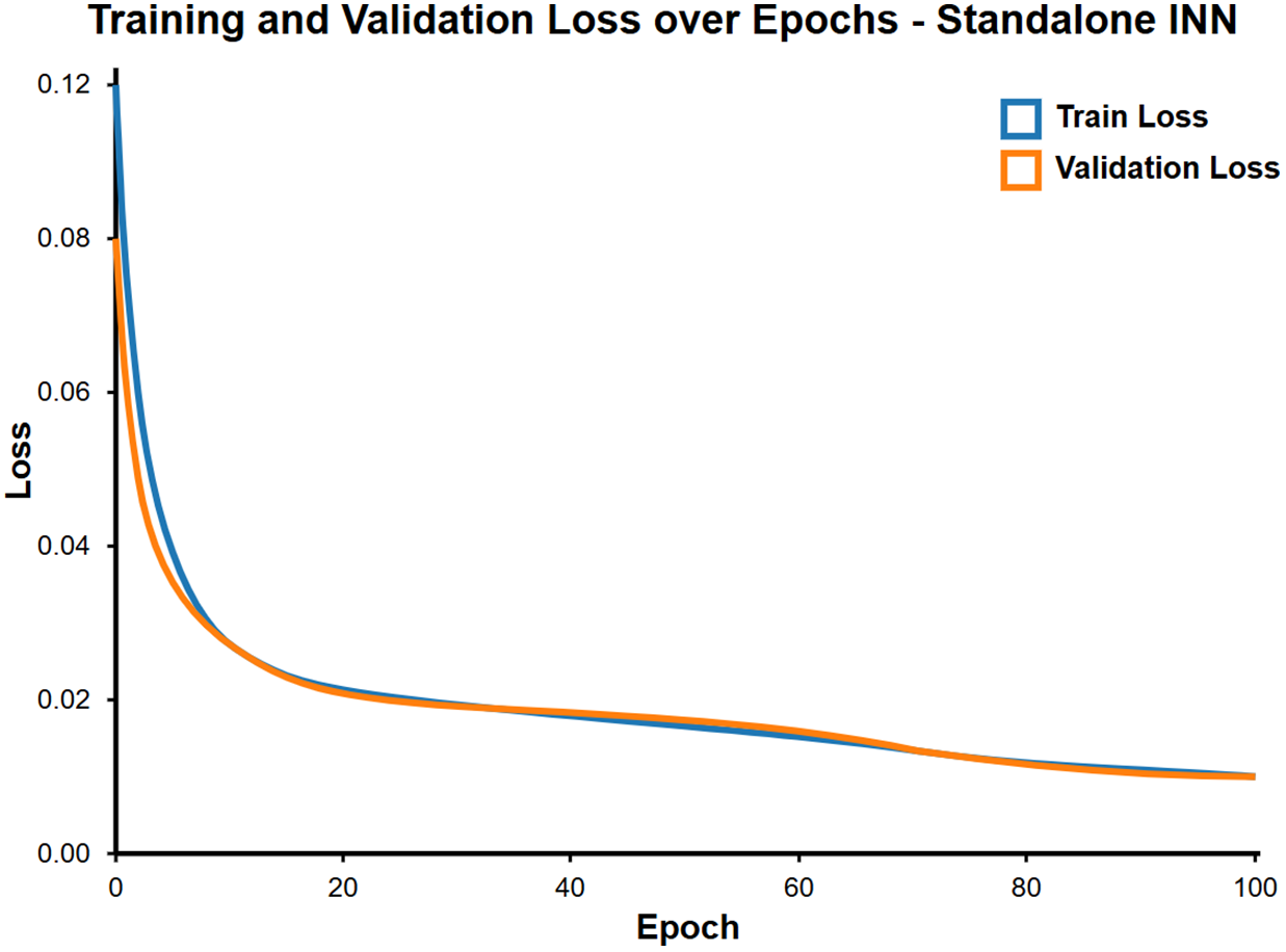
Figure 8: Training and validation loss curves over 100 epochs for the Standalone INN model. The train and validation loss decrease rapidly in the first 20 epochs and stabilize at low values, indicating effective learning by the model. The minimal gap between the training loss and validation loss throughout the training process suggests that the model generalizes well without overfitting
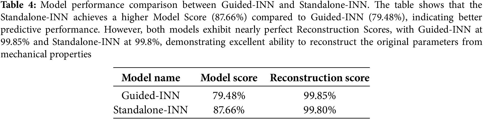
The R2 score on the INN itself is called the ‘Model Score’, while the R2 score of the geometries generated through the FNN is called the ‘Reconstruction Score’, as shown in Fig. 9. Table 4 provides a comparison.
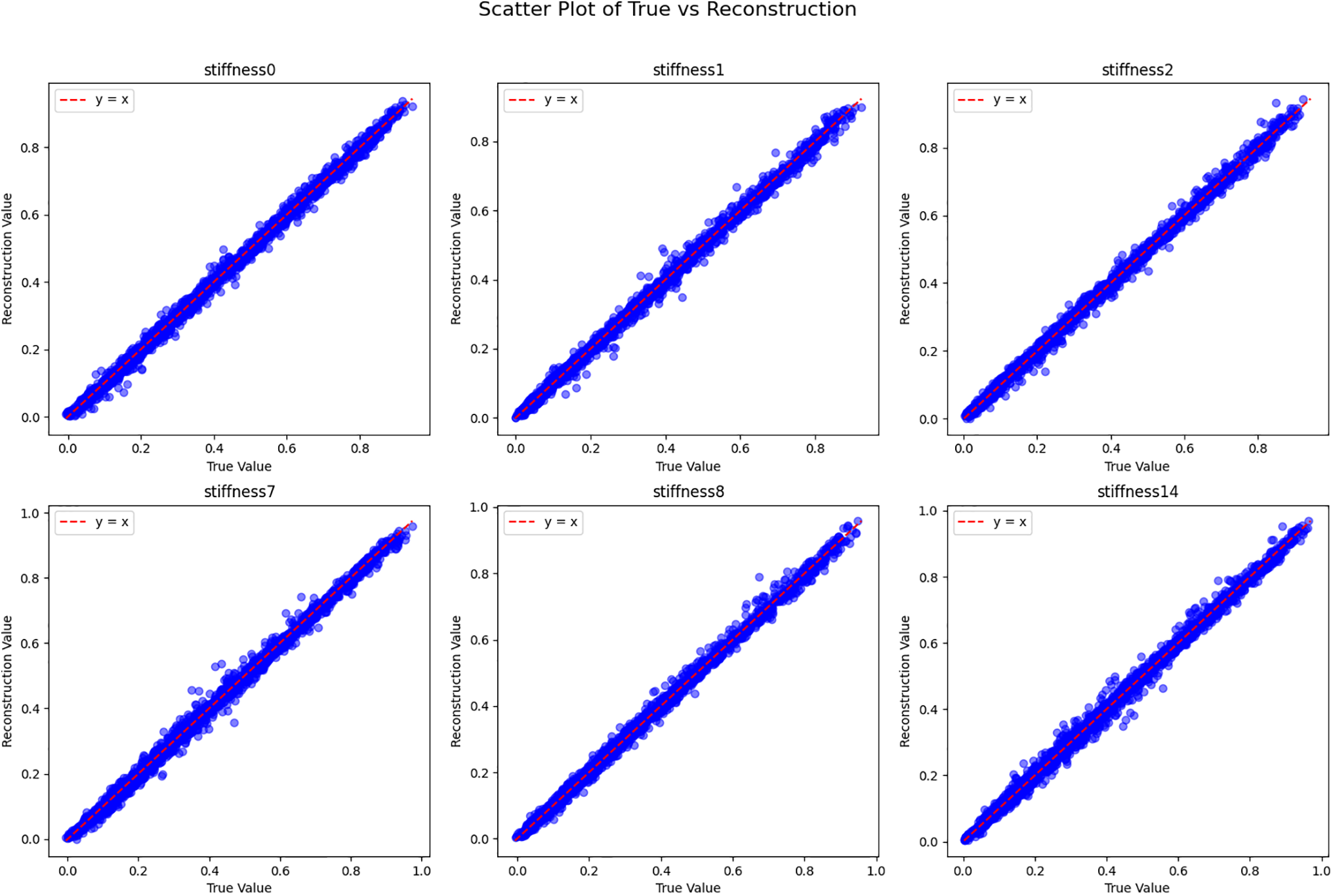
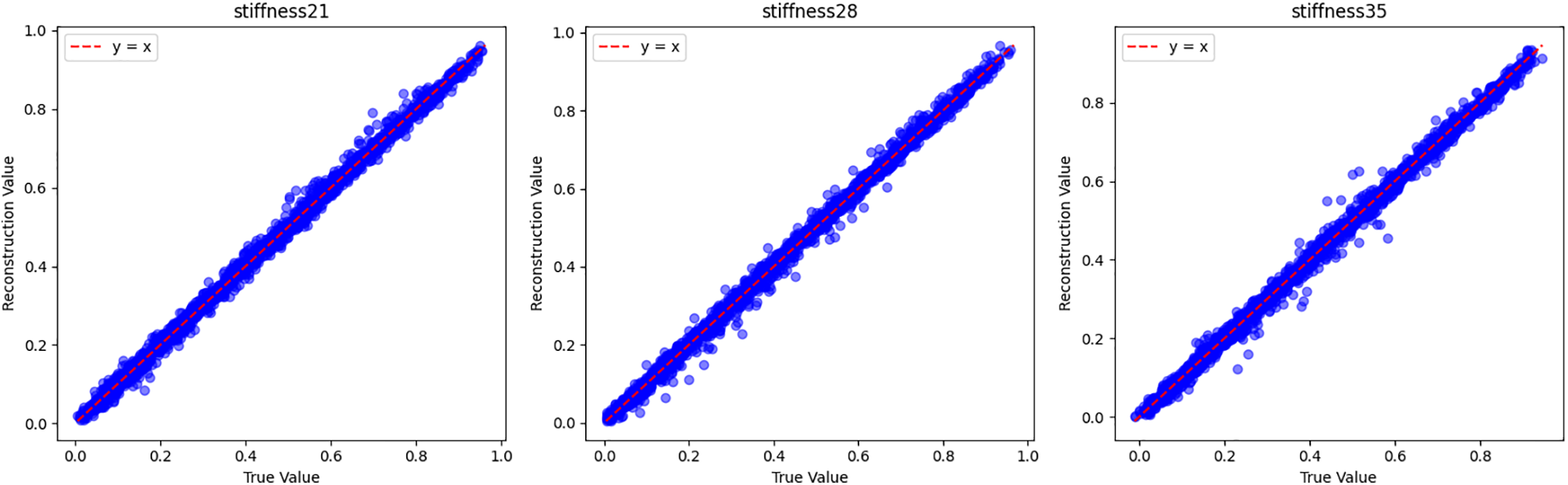
Figure 9: Scatter plots of true vs. reconstructed values for various stiffness parameters with an R2 reconstruction score of 99.8%. Each scatter plot compares the true stiffness values (x-axis) with the corresponding reconstructed values (y-axis) for different stiffness parameters (stiffness0, stiffness1, etc.). The data points align closely with the y = x line (red dashed line), indicating an almost perfect reconstruction of the stiffness values. The high R2 score of 99.8% further supports the accuracy and reliability of the reconstruction model, demonstrating its ability to capture nearly all of the variance in the true values
Results of Standalone-INN: The results demonstrate that training an independent INN without the support of an FNN is entirely feasible. The “independent INN” can still generate geometries that meet the required mechanical properties accurately without needing the FNN’s guidance during training. This shows that focus on training the INN independently, reducing complexity, and saving computational resources.
4.1.1 Independent-INN-Gaussian Network
An advancement of the “independent INN” network involves adding a Gaussian noise mechanism during the training process. Typically, adding noise to a Multilayer Perceptron (MLP) reduces accuracy, but since the “independent INN” has already achieved a much higher R2 score than the Guided-INN, this negative impact has been mitigated. The “independent INN-Gaussian” network is designed to generate multiple geometries in the form of modeling parameters from a single set of mechanical properties. This is equivalent to solving the data generation problem, similar to Generative Adversarial Networks (GAN) or Variational Autoencoders (VAE), but without the need for the presence of the FNN.
In models like VAE and GAN, the FNN often plays an important supporting role. In VAE, the FNN functions as a decoder to guide the encoder in encoding the data. In GAN, the FNN acts as a discriminator, evaluating and classifying the results generated by the generator network. However, the interesting distinction of the “independent INN-Gaussian” is that it does not require the participation of the FNN during the training process.
This approach incorporates Gaussian noise into the “independent INN” as follows: Gaussian noise is added during training, with standard deviation (σ) as a key component, as shown in Fig. 10. The higher the value of σ, the greater the variability in the data and the differences between the predictions. This allows the “independent INN-Gaussian” to function as a generative network similar to VAE or GAN, but with a different approach. By adding Gaussian noise, the “independent INN-Gaussian” can generate multiple geometry versions from the same mechanical property set, extending its generalization ability and creating diverse data without the need for FNN guidance.
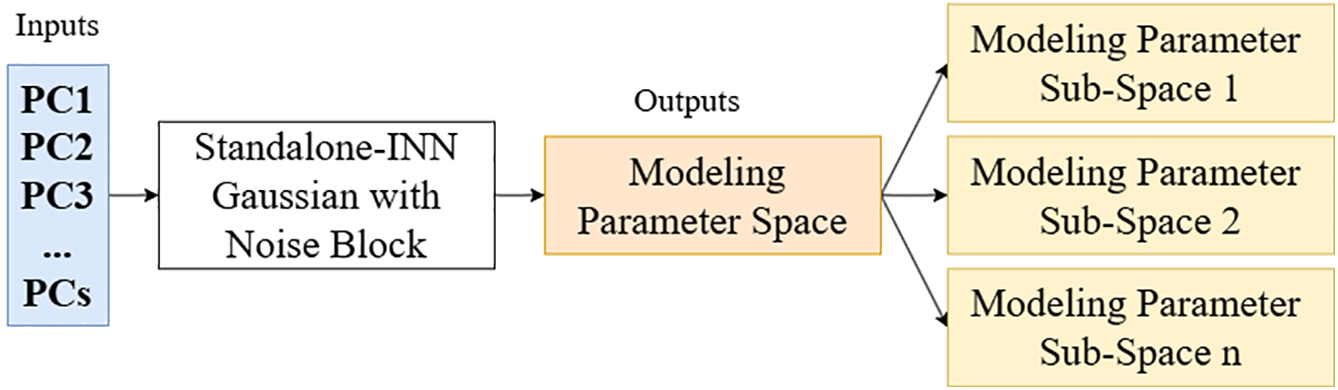
Figure 10: Architecture of the Standalone INN-Gaussian with Noise Block for generative modeling of parameters. The model takes Principal Components (PCs) as input and passes them through the Standalone INN with a Gaussian Noise Block. This block introduces Gaussian noise during training, allowing the model to generate multiple variations of modeling parameters for each input set of mechanical properties. The output consists of a modeling parameter space that is further divided into multiple sub-spaces, each representing different potential geometries corresponding to the same set of mechanical properties. This architecture enables the Standalone INN-Gaussian network to act as a generative model, similar to Variational Autoencoders (VAE) or Generative Adversarial Networks (GAN), but without the need for an FNN during the training process
As shown in Fig. 10, the Standalone INN-Gaussian framework incorporates controlled Gaussian noise during inference to generate diverse geometries while maintaining accuracy. The mathematical formulation is as follows:
1. Noise Injection—Given input features X (mechanical properties and/or latent features), we add noise:
where σ is a tunable standard deviation controlling diversity.
2. Geometry Generation—The noisy input X′ is passed through the pre-trained Standalone INN:
where m′ is the generated modeling parameter set.
3. Quality Control—This step can be performed if there is previous FNN training or another equivalent method to validate the m′ results:
The deviation from the target properties
where ϵ is a user-defined tolerance (e.g., ϵ = 0.05 for 5% error).
The similarity of this Gaussian noise block has the same working mechanism as VAE or GAN, as described in Fig. 11, and by tuning σ and ϵ, balance diversity and accuracy (Figs. 12–15).
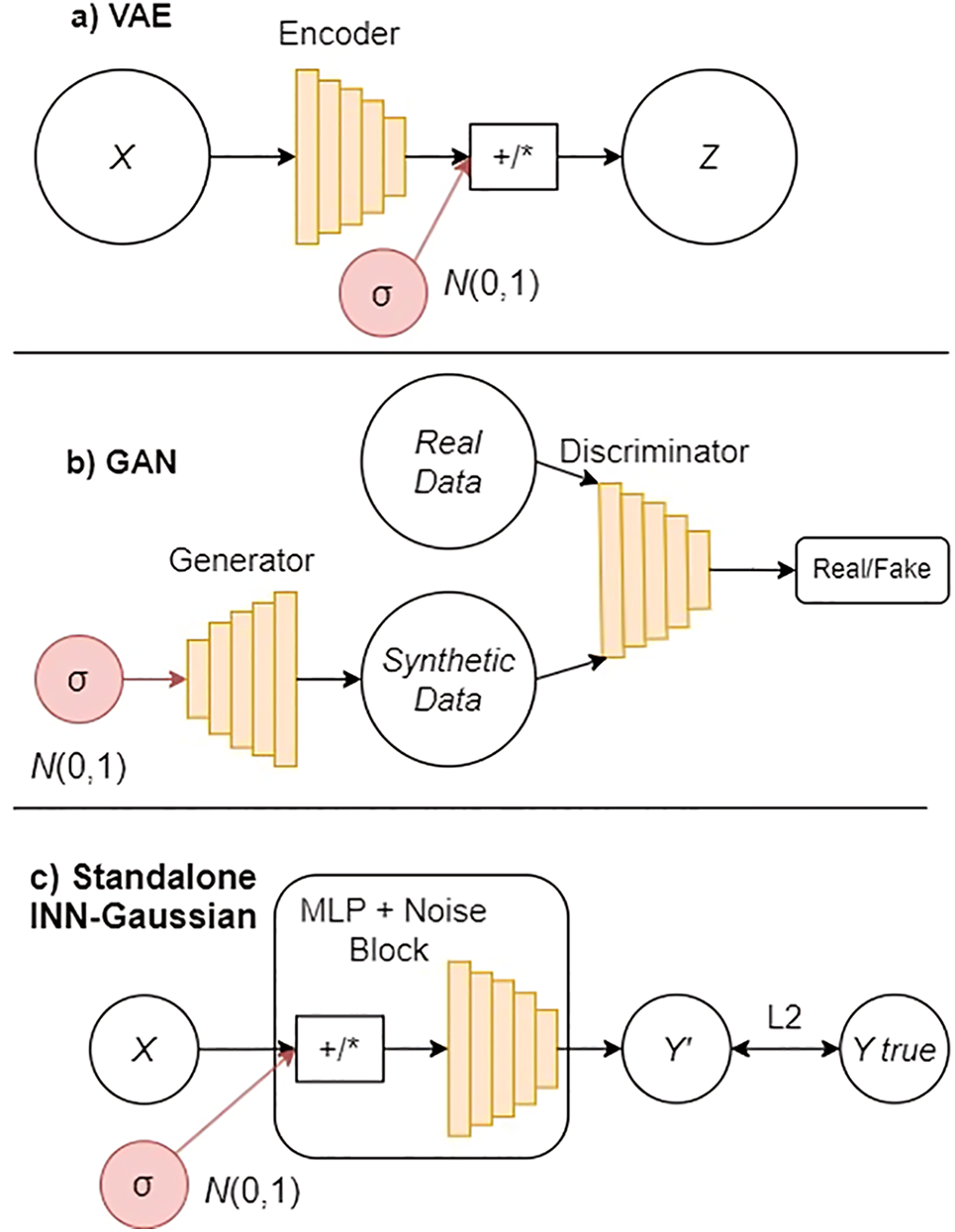
Figure 11: Comparison of VAE, GAN, and Standalone INN-Gaussian architectures incorporating Gaussian noise. (a) VAE (Variational Autoencoder): The model introduces Gaussian noise N(0, 1) with standard deviation σ in the encoding process. The noise is combined with the encoded data to generate the latent variable Z, which is then decoded to reconstruct the input data. (b) GAN (Generative Adversarial Network): The generator network creates synthetic data, starting by adding Gaussian noise N(0, 1). The discriminator network then evaluates the generated data to classify it as real or fake. This process is iterative and adversarial. (c) Standalone INN-Gaussian-ours method: The model introduces Gaussian noise N(0, 1) into the Multilayer Perceptron (MLP) block during training. The noise is added to the input X to generate a predicted output Y′, which is compared to the true value Y_true using an L2 loss function. Unlike the VAE and GAN models, the Standalone INN-Gaussian does not rely on an FNN for guidance, making it independent during the training process
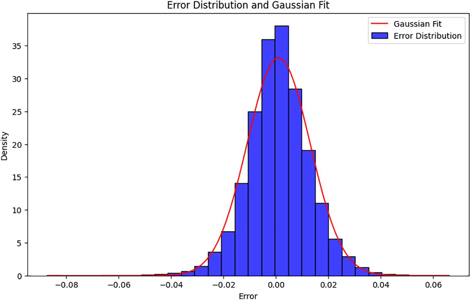
Figure 12: Error distribution and Gaussian fit for the Standalone INN-Gaussian model. With an initial Gaussian noise σ = 0.005, the model generates diverse modeling parameters. The mechanical properties predicted by the FNN, resulting in a slight error of 0.1%–0.2%. The error distribution closely follows a Gaussian fit, indicating the model’s ability to generate diverse yet accurate geometry samples without FNN guidance
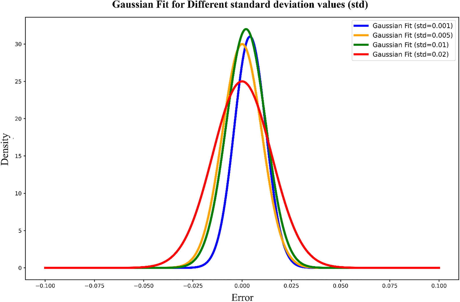
Figure 13: Gaussian fit for different standard deviation values of noise in the Standalone INN-Gaussian model. The plot compares error distributions for various noise standard deviations (σ = 0.001, 0.005, 0.01, and 0.02). As σ increases, the error distribution widens, reflecting greater variability in the generated data. This shows how noise impacts the diversity and accuracy of the generated modeling parameters, with smaller σ values resulting in more concentrated and accurate predictions, while larger σ values introduce more variability
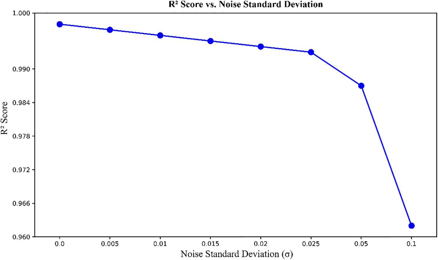
Figure 14: R2 score vs. noise standard deviation (σ) in the Standalone INN-Gaussian model. The plot shows the relationship between the R2 score and increasing levels of σ. As σ increases, the R2 score gradually decreases, indicating a reduction in prediction accuracy. However, even with higher levels of noise, the model maintains a high R2 score above 0.965, demonstrating its robustness in generating accurate predictions despite the introduction of variability. The elbow point around σ = 0.02 to 0.03 represents the most beneficial noise level, where the model maintains high accuracy (R2 score) while still incorporating variability from Gaussian noise
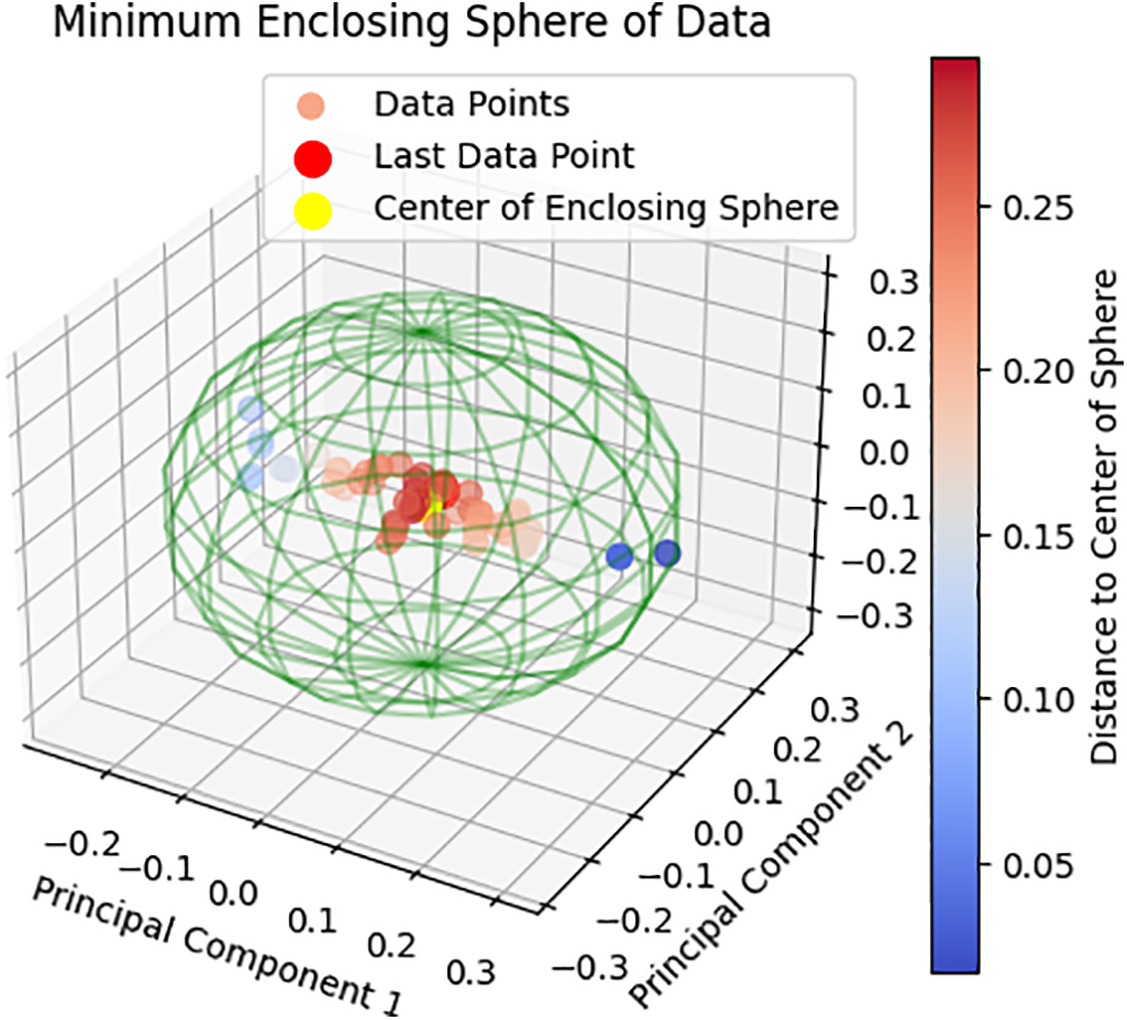
Figure 15: Visualization of mechanical properties generated from variants of modeling parameters using Standalone INN-Gaussian-ours method. In the plots, the ‘Last Data Point’ represents the reference sample without Gaussian noise, while the surrounding points show variants generated with Gaussian noise. These points are distributed around the reference following a Gaussian distribution, as seen in both 3D visualizations. The red dot represents the center of the Gaussian distribution, and the distance of each sample to this center is reflected by the color bar
4.1.2 Similarities with VAE and GAN
Gaussian Noise and Randomness:
• In the “independent INN-Gaussian”, Gaussian noise is added to the input before passing it through the model. This means that each forward pass with the same mechanical property value can generate a different geometry value.
• This approach is similar to VAE, where after encoding the input into a latent space, noise is added to create a set of random points in that space, from which different variations of the output are decoded.
• GAN also employs a random data generation mechanism through Gaussian noise as input to the generator network to create new data samples. This noise determines the characteristics of the generated data sample, leading to diversity in the output data versions.
Adjusting the Degree of Variation:
• In the “independent INN-Gaussian”, σ serves as a component that adjusts the uncertainty. When the value of σ is large, the variability in the geometries generated from the same mechanical property also increases. This allows control over the diversity of the generated geometries.
• In GAN, a similar mechanism is applied by adjusting the intensity of the noise input to the generator. This noise determines the diversity of the generated data samples, similar to the role of σ in the “independent INN-Gaussian”.
Randomness in Predictions:
• Like VAE and GAN, the “independent INN-Gaussian” model with Gaussian noise allows generating multiple random results from the same mechanical property input. This is useful in problems that do not require a single predicted value, but rather require a distribution or set of possible values, as shown Fig. 11.
With an initial σ value of 0.005, the “independent INN-Gaussian” learns to generate different modeling parameters, and the mechanical properties measured R2 score by the FNN are: (0.9968, 0.9974, 0.9975, 0.9969, 0.9975, 0.9972, 0.9974, 0.9974, 0.9972). Although accuracy decreases slightly (around 0.1%–0.2%), the model still maintains high-quality data generation. This error is represented as an error spectrum reflecting the Gaussian distribution during the data generation process of the “independent INN-Gaussian”, as shown in Fig. 12. This indicates that the “independent INN-Gaussian” model can generate diverse geometry samples while still meeting the requirements for mechanical properties, similar to what VAE and GAN accomplish, but without the need for FNN guidance.
Overview of the data generation capability of Standalone-INN-Gaussian:
• Stability and Accuracy: With a σ value of 0.005, the independent INN-Gaussian demonstrates that adding randomness to the generation process of the modeling parameters does not significantly reduce the accuracy of the mechanical properties. This shows that the model can maintain stability in data generation, even with slight variations due to Gaussian noise. As a result, the independent INN-Gaussian can generate modeling parameters with a reasonable degree of randomness while still meeting the requirements for mechanical properties.
• Reasonable Randomness: The level of randomness added to the modeling parameters through Gaussian noise still preserves the stability of the mechanical properties. This indicates that the independent INN-Gaussian can be used to generate modeling parameter values close to the actual values while ensuring a certain level of diversity. This model can create different geometry samples from the same mechanical property, which is very useful for studying variations in material design.
• Potential for Data Generation: Gradually increasing the value of σ allows the independent INN-Gaussian to learn how to generate progressively different modeling parameters, thus identifying the threshold of variation while still controlling the desired mechanical precision.
To optimize the data generation process, systematic evaluations with different σ values of need to be carried out to assess their impact on the error spectrum of mechanical properties. Through experimentation and observation, an appropriate σ value can be determined to ensure a balance between the diversity of the generated modeling parameters and the precision of the required mechanical properties, as shown in Fig. 13. Choosing the correct σ value helps optimize the data generation capability of the ‘independent INN-Gaussian’, better serving problems that require generating multiple geometry versions while meeting mechanical property criteria.
The elbow method is a useful tool for determining the optimal value of σ during the training process of the independent INN-Gaussian model. The elbow point represents the position where the improvement in the model’s performance starts to plateau, meaning that further increasing σ no longer provides significant benefits or even leads to a decline in performance. Identifying the correct elbow point helps balance the noise for generating diverse data while maintaining prediction accuracy, as shown in Fig. 14.
Analysis of the Graph:
Initial stage (σ from 0 to around 0.02):
• For σ values less than 0.02, the R2 score remains high with a very slight decrease, almost negligible. This indicates that adding a small amount of noise to the data generation process of modeling parameters does not significantly affect the accuracy of the mechanical properties.
• At this stage, the model maintains stability and accuracy while adding the necessary randomness to create different geometry versions from the same mechanical property. This is crucial for applications requiring result diversification without sacrificing quality.
After the elbow point (σ from around 0.03 and above):
• From σ = 0.03, the R2 score begins to decline at a faster rate. This indicates that adding too much noise reduces the ability to accurately reproduce the desired mechanical properties.
• The noticeable performance decline after the elbow point suggests that the model starts to lose the ability to maintain a close correlation between the modeling parameters and mechanical properties, leading to a reduction in the quality of the prediction. Adding too much noise can cause the model to become too random, resulting in instability during the prediction process.
Determining the Elbow Point:
• The elbow point is identified around σ = 0.02. This is the position where the rate of decline of the R2 score begins to increase, signaling that further increasing σ no longer provides significant benefits, but instead leads to a decrease in performance.
• Before this point, the decrease in the R2 score is minimal, almost negligible. This allows the use of randomness in data generation without significantly affecting mechanical properties. After this point, the R2 score declines sharply, indicating that adding more noise will lead to a considerable performance decrease.
Based on the elbow method, the σ value of 0.02 is the optimal choice for the ‘independent INN-Gaussian’ model. At this value, the model can generate diverse geometries while maintaining a high R2 score, ensuring the accuracy of the desired mechanical properties, as shown in Fig. 15. This is crucial in inverse design applications, where it is necessary to maintain a balance between the diversity of generated data and the accuracy of predictions. Increasing σ beyond 0.02 leads to a significant decline in prediction quality, making this elbow point an important boundary to optimize the data generation process without compromising the model’s accuracy.
Following the study of Ha et al., 2023 [58], the data set for this problem consists of 280 rows, each describing the material response under loading through characteristic parameters of the stress-strain curve. These parameters include:
• U_loading [N/m2]: Represents the applied stress or load to which the material is subjected, measured in Newtons per square meter (N/m2) or Pascals (Pa).
• S_linear [Pa]: The stress at the end of the linear region of the curve, indicating the phase where the material still follows the ideal elasticity according to Hooke’s law.
• eps_linear [-]: Deformation at the end of the linear region, dimensionless, indicating the level of strain the material undergoes in the elastic region.
• S_local_max [Pa] and eps_local_max [-]: Local maximum stress and corresponding strain, respectively, which identify the highest stress the material withstands before it begins to unload.
• S_local_min [Pa] and eps_local_min [-]: Local minimum stress and strain, often related to phenomena like cracking or plastic deformation.
• S_end [Pa] and eps_end [-]: Stress and strain at the final point of the test, typically when the material fails or the test ends, reflecting the material’s endurance and tensile strength.
Additionally, the data set includes three parameters related to the geometric structure Tgene, angle [deg], and r1/L1 [-]:
• Tgene: A parameter describing the material’s structural characteristics and influencing its overall mechanical properties.
• angle [deg]: An angle measured in degrees related to the geometric structure affecting the orientation and arrangement of fibers or layers in the material.
• r1/L1 [-]: A size ratio that describes the geometric relationship within the material’s structure and influences how the material responds to loading.
These parameters allow for a detailed description of the mechanical behavior under loading and show the dependence of mechanical properties on the material’s geometric structure of the material, as shown in Fig. 16.
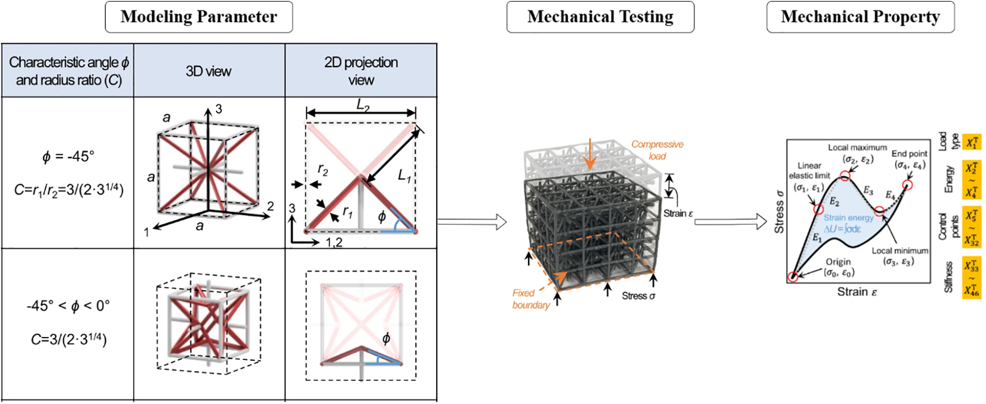
Figure 16: Ha et al.’s [58] parameter modeling process as benchmark data in study 2
The original data set consists of 280 rows with a one-to-one mapping between geometry (in the form of modeling parameters) and mechanical properties, specifically the stress-strain curve. This means that each geometry corresponds to a unique mechanical property and vice versa. Although in theory, the relationship between geometry and mechanical properties can be one-to-many or many-to-many, within the scope of this dataset and the study hypothesis, assuming a one-to-one relationship is reasonable.
Research Implementation Steps:
Step 1: Generate data using transformations based on Mechanical Theory
• The data set is expanded from 280 rows to 2808 rows through transformations, including creating new features based on the available information. Some new features are created using one-hot encoding for categorical data types, while others are derived through calculations and conditions.
• From the initial nine mechanical property parameters, the data are expanded into nine mechanical property parameters and four geometric parameters.
• From the initial three geometry parameters, the data are expanded into seven parameters.
Step 2: Create FNN_curvetype
• The FNN_curvetype network is trained to learn the mapping from seven geometric parameters to four geometric parameters.
• The precision of this network is evaluated using the R2 score, reaching 93.5%, indicating its ability to learn and predict the relationship between geometry and geometric parameters effectively.
Step 3: Create FNN_points
• The FNN_points network is trained to learn the mapping from seven geometry parameters to nine mechanical property parameters.
• The accuracy of FNN_points achieves an R2 score of 97.53%, demonstrating its strong ability to predict mechanical property parameters based on geometry.
Step 4: Create an INN Network involving both FNN_curvetype and FNN_points
• The INN network is designed with an input consisting of nine mechanical property parameters and four geometric parameters, while the output comprises seven geometric parameters. Among the seven outputs, five are in the form of one-hot encoded categories.
• The INN network training process uses both FNN_curvetype and FNN_points to improve the mapping between the parameters. FNN_curvetype assists in mapping from geometry to geometric parameters, while FNN_points handles mapping from geometry to mechanical properties.
Using this approach, the study utilizes the one-to-one relationship in the original dataset to expand and build deep learning models such as FNN and INN. This helps to better understand the relationship between geometry and mechanical properties and enhances the ability to predict and generate data in inverse design problems.
In this study, the focus is not on optimizing the performance of the INN itself but on testing the ability of the seven geometry parameters generated by the INN to reconstruct the stress-strain curve when fed into two FNN networks: FNN_curvetype and FNN_points, as shown in Fig. 17. The goal is to ensure that the Normalized Root Mean Squared Error (NRMSE) of this stress-strain curve is sufficiently small to demonstrate the effectiveness of the Standalone_INN. To achieve this, a standalone INN network was constructed without involving any FNN networks during the training process, as shown in Fig. 18.
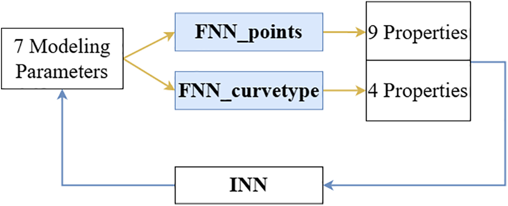
Figure 17: Traditional model structure using an INN and two FNNs. The INN generates 7 modeling parameters, which are then evaluated by two separate FNNs: FNN_points, responsible for predicting 9 mechanical properties, FNN_curvetype, responsible for predicting 4 additional properties based on the curve type. These properties are used to evaluate and validate the modeling parameters generated by the INN, ensuring the model’s performance for different property sets
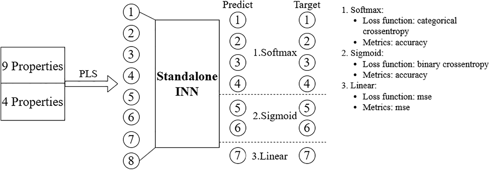
Figure 18: Architecture of the Standalone INN-our method model using PLS components for multi-task predictions. The model takes 9 and 4 mechanical properties as input, which are reduced to 8 PLS components using Partial Least Squares (PLS). These components are fed into the Standalone INN to generate predictions across different tasks. Outputs 1–5 use the softmax activation for multi-class classification (evaluated with categorical crossentropy and accuracy metrics), output 6 uses sigmoid for binary classification (evaluated with binary crossentropy and accuracy), and output 7 uses linear activation for regression (evaluated with mean squared error (MSE))
NRMSE, a common way of measuring the quality of the fit the model, given by:
where
The detailed procedure consists of three main steps:
Step 1: Identify Significant Components as Input for Standalone_INN
• Using PLS: Unlike Study 1, this study selects the partial least squares (PLS) method to analyze the relationship between the 13 input features of the INN and the seven outputs. PLS is used to find the components that have the strongest correlation with the outputs, helping Standalone_INN focus on the most meaningful features.
• Selecting PLS Components: From the correlation table between the 13 PLS components and the seven outputs, the study determined that the last four PLS components have very weak correlations (in the range of −0.2 < x < 0.2) with the outputs, as shown in Fig. 19. Therefore, these four components were excluded, and the first eight PLS components were retained as input for Standalone_INN. This ensures that Standalone_INN uses only the input features closely related to the outputs.
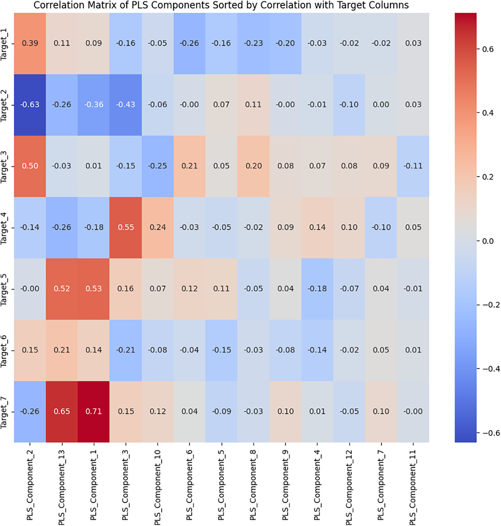
Figure 19: Correlation matrix of PLS components sorted by their correlation with target columns. The heatmap shows the correlation between each of the PLS components and the seven targets. PLS components were selected based on their correlation strength with the targets, as seen by the darker shades of red and blue. The first 8 PLS components were chosen for further modeling due to their higher correlation with multiple targets, ensuring that key information is retained while reducing dimensionality
Step 2: Construct an Appropriate Standalone_INN Network
• Network Design: Standalone_INN is specifically designed to handle seven outputs with different properties. To achieve this, the network uses three different output types, each employing a separate activation function and loss function.
• Reason for Complex Design: Since the seven outputs of the INN include various data types, such as one-hot encoded categorical variables and continuous variables, using multiple activation functions and loss functions helps the model learn and predict more accurately. This design ensures that Standalone_INN can process various types of information during learning.
Step 3: Evaluate the Capability of Standalone_INN
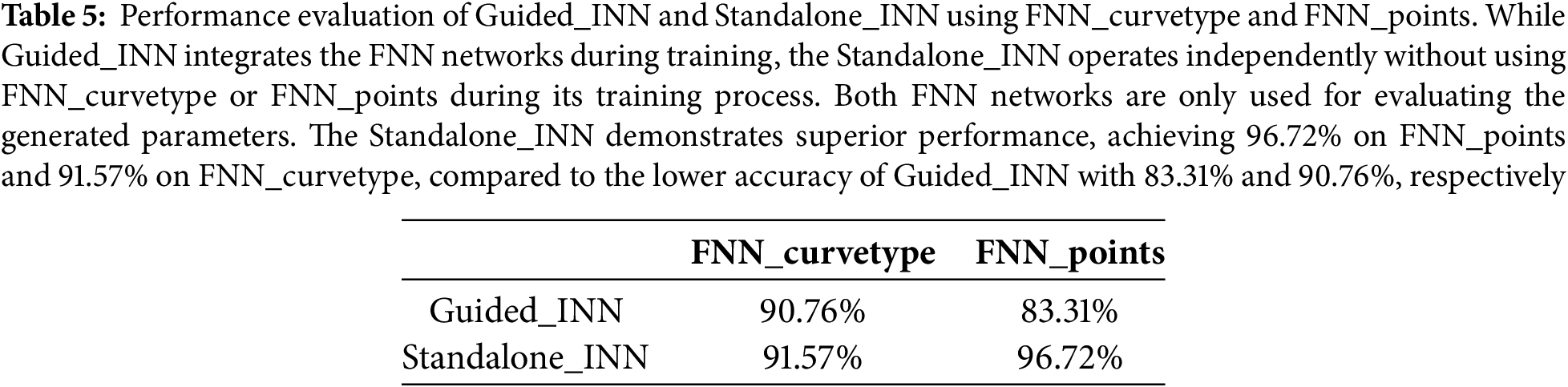
• Evaluation Using the R2 Score: To assess the performance of Standalone_INN, the geometry parameters generated by Standalone_INN were passed through FNN_curvetype and FNN_points. The goal was to test the ability to reconstruct the stress-strain curve. Standalone_INN achieved an R2 score of 96.7% for reconstructing the physical parameters and 90.76% for the curvetype, as presented in Table 5.
• Comparison with FNN-Guided INN: This result shows that Standalone_INN outperforms the INN guided by FNN. This proves that Standalone_INN, when constructed and optimized correctly, can effectively reconstruct geometry without the support of FNN networks during training.
5.1 Performance Analysis and Comparative Evaluation
This study demonstrates the feasibility and superior performance of standalone INN for metamaterial inverse design, achieving significant computational advantages while maintaining high reconstruction accuracy. The standalone INN architecture achieved 99.8% reconstruction accuracy for stiffness parameters in Study Model 1, representing an 8.18% improvement over guided-INN approaches. In Study Model 2, the standalone framework demonstrated 96.72% accuracy, substantially outperforming guided-INN approaches. These results align with recent findings in metamaterial inverse design research.
5.2 Comparative Analysis with Existing Methods
The integration of PCA and PLS dimensionality reduction techniques in our standalone INN framework addresses critical limitations in current methodologies. Compared to generative approaches (GANs, VAEs), our standalone INN-Gaussian methodology provides distinct advantages: eliminating dependencies on discriminator networks/encoder-decoder architectures while maintaining equal/superior accuracy and enabling diverse geometry generation through Gaussian noise injection.
5.3 Challenges and Limitations in Complex Geometry Optimization
Despite these strengths, scalability remains a significant challenge, particularly when moving from laboratory-scale prototypes to industrial manufacturing. Furthermore, while the one-to-one relationship assumption between geometry and mechanical properties holds for the datasets used here, real-world scenarios often involve many-to-one or one-to-many relationships due to measurement uncertainties and environmental variability. The need for validated numerical datasets also restricts the approach’s applicability to contexts where comprehensive data are available. Additionally, although Gaussian noise integration enables geometric diversity, it introduces a trade-off: as the noise parameter σ exceeds 0.02, reconstruction performance declines, limiting the range of viable design exploration.
5.4 Future Applications and Extensions
Future research should extend beyond current one-to-one mappings to address one-to-many and many-to-many relationships. Integrating advanced manufacturing simulation tools could allow fabrication constraints to be considered directly within the optimization process. Moreover, the framework’s adaptability for transfer learning across diverse material domains presents promising opportunities to accelerate AI-driven discovery in areas ranging from electronic materials to biomedical devices.
This study demonstrates that a standalone INN framework can deliver highly accurate and computationally efficient solutions for metamaterial inverse design. By leveraging PCA-PLS dimensionality reduction and eliminating the need for FNNs, the proposed approach achieves state-of-the-art reconstruction accuracy while enabling diverse geometry generation through Gaussian noise integration.
Although the method is currently limited by the assumption of a one-to-one relationship between geometry and mechanical properties, and by the availability of comprehensive datasets, it provides a robust foundation for future work. Expanding the methodology to handle more complex relationships and integrating manufacturing constraints will further enhance its applicability, positioning this framework as a versatile tool for next-generation AI-driven materials discovery.
Acknowledgement: Authors would like to thank the Deutsche Forschungsgemeinschaft (DFG, German Research Foundation) for supporting this research under Germany’s Excellence Strategy within the Cluster of Excellence PhoenixD (EXC 2122, Project ID 390833453).
Funding Statement: Nguyen Dong Phuong and Xiaoying Zhuang appreciate the funding by the Deutsche Forschungsgemeinschaft under Germany’s Excellence Strategy within the Cluster of Excellence PhoenixD (EXC 2122, Project ID 390833453).
Author Contributions: Conceptualization, Nguyen Dong Phuong and Nanthakumar Srivilliputtur Subbiah; methodology, Nguyen Dong Phuong; software, Nguyen Dong Phuong; validation, Nguyen Dong Phuong, Nanthakumar Srivilliputtur Subbiah and Yabin Jin; formal analysis, Nguyen Dong Phuong and Yabin Jin; investigation, Nguyen Dong Phuong; resources, Xiaoying Zhuang; data curation, Nguyen Dong Phuong; writing—original draft preparation, Nguyen Dong Phuong; writing—review and editing, Nguyen Dong Phuong, Nanthakumar Srivilliputtur Subbiah, Yabin Jin and Xiaoying Zhuang; visualization, Nguyen Dong Phuong; supervision, Nanthakumar Srivilliputtur Subbiah and Xiaoying Zhuang; project administration, Xiaoying Zhuang; funding acquisition, Xiaoying Zhuang. All authors reviewed the results and approved the final version of the manuscript.
Availability of Data and Materials: The datasets generated and/or analyzed the current study are available from the corresponding author on reasonable request.
Ethics Approval: Not applicable.
Conflicts of Interest: The authors declare no conflicts of interest to report regarding the present study.
Abbreviations
| Abbreviation | Full Term |
| AI | Artificial Intelligence |
| CAD | Computer-Aided Design |
| FEM | Finite Element Method |
| FNN | Feedforward Neural Network |
| GAN | Generative Adversarial Network |
| INN | Inverse Neural Network |
| MLP | Multilayer Perceptron |
| MSE | Mean Squared Error |
| NMSE | Normalized Mean Squared Error |
| PCA | Principal Component Analysis |
| PLS | Partial Least Squares |
| R2 | Coefficient of Determination |
| VAE | Variational Autoencoder |
| IQR | Interquartile Range |
| Adam | Adaptive Moment Estimation |
| ReLU | Rectified Linear Unit |
| z-score | Standard Score Normalization |
This appendix provides detailed supplementary information to support transparency, reproducibility, and rigorous evaluation of the study. The materials herein are intended to complement the main manuscript by offering in-depth descriptions, technical clarifications, and practical resources related to the datasets, data preprocessing, model architecture, training procedures, hyperparameter configurations, evaluation protocols, and reproducibility assets.
Key objectives of this appendix are:
• To describe fully the datasets utilized, including their structure, preprocessing steps, and suitability for the modeling approaches chosen (Appendix B).
• To elaborate on the dimensionality reduction processes, feature engineering strategies, and rationale behind these methodological choices (Appendix C).
• To document the precise architecture and training pipeline of the standalone inverse neural network (INN) models, accompanied by code-style pseudocode for key procedures (Appendix D).
• To summarize all hyperparameters, experimental design parameters, and evaluation metrics, ensuring that results can be accurately reproduced and interpreted (Appendixs E and F).
By systematically organizing these supplementary materials, we aim to enhance the clarity of the methodological framework and facilitate independent validation or extension by the broader community.
Appendix B Dataset Descriptions & Preprocessing
This section describes the two datasets used (Kumar et al., 2020 [57]; Ha et al., 2023 [58]), details each preprocessing step, explains how these steps support dimensionality reduction (Appendix C) and standalone INN training (Appendix D).
Appendix B.1 Kumar et al., 2020 Dataset [57]
The Kumar et al. 2020 dataset [57] serves as the primary validation benchmark for the proposed inverse design framework in this study (case 1). This dataset encompasses material samples specifically designed to exhibit a clear one-to-one relationship between geometric parameters and mechanical properties, making it particularly suitable for PCA-based dimens.
Appendix B.1.1 Structural Overview
1. Sample count: 12,582 unique unit-cell designs.
2. Geometry descriptor vector m (ℝ4):
3. volFrac—relative solid volume fraction (continuous, 0–1).
4. thetaX—rotation about x-axis (continuous, −90°–+90°).
5. thetaY—rotation about y-axis (continuous, −90°–+90°).
thetaZ—rotation about z-axis (continuous, −90°–+90°).
Mechanical property vector y (ℝ9): full stiffness tensor (symmetry-reduced Voigt form).
Appendix B.1.2 Pre-Processing Pipeline
• Consistency Check: Remove duplicates to ensure each (m, y) pair is unique, which is essential for the INN to learn a valid inverse.
• Z-Score Normalization: Standardize all nine mechanical properties to zero mean and unit variance. This prevents any single dimension from dominating PCA and stabilizes network training.
• Outlier Removal: Exclude 27 samples with extreme z-scores to avoid gradient explosions while retaining sufficient diversity.
• Stratified Split: Cluster samples by their top principal components of y, then split into train/val/test sets (60/20/20) with seed 42. This ensures each subset mirrors the overall property distribution, supporting both INN training (Appendix D) and fair evaluation.
Appendix B.2 Ha et al., 2023 Dataset [58]
The Ha dataset [58] contains 2808 samples, each with five continuous geometry features and two categorical features. After one-hot encoding, the geometry vector expands to eight binary features. Targets include thirteen mechanical properties (elastic moduli, shear moduli, Poisson ratios, yield strength). The complex, nonlinear mapping motivates a covariance-aware reduction method (PLS, Appendix C.1).
Appendix B.2.1 Structural Overview
• Sample count: 2808 metamaterial designs.
• Geometry descriptor vector m (ℝ7):
• 5 continuous parameters.
• 2 categorical parameters → expanded to 8 one-hot binary features after encoding.
• Mechanical property vector y (ℝ13): elastic modulus, shear modulus in three planes, Poisson ratios, and yield strength metrics.
Appendix B.2.2 Pre-Processing Pipeline
1. Missing values—0.3% of property entries imputed via k-nearest neighbours (k = 5) within the same lattice type to maintain physical plausibility.
2. Categorical encoding—topology & boundary layer converted to one-hot (8 binary columns), appended to the 5 continuous geometry features (total q = 13).
3. Continuous scaling—min-max (0, 1) normalisation for continuous geometry; z-score for mechanical properties to balance variance.
4. Train/val/test split—stratified by topology class (8 categories), 60/20/20, seed = 42.
Appendix B.3 Preprocessing Footprint Summary
Each preprocessing step—from duplicate removal to latent-space construction—was chosen to enhance PCA or PLS performance (Appendix C) and to provide a robust, reproducible foundation for standalone INN training (Appendix D).
Appendix C Dimensionality Reduction & Feature Engineering
This section describes the two primary latent space construction techniques—Principal Component Analysis (PCA) and Partial Least Squares (PLS), used in this study to facilitate efficient and robust inverse design model training. Each method is justified in context of both the datasets’ characteristics and the requirements of the standalone inverse neural network (INN) framework.
Appendix C.1 Principal Component Analysis (PCA)
Objective:
Reduce the dimensionality of the mechanical property vector
Procedure:
1. Standardize the training property data matrix
2. Compute the empirical covariance matrix:
3. Perform eigendecomposition of
where
4. Select the minimum number of principal components
5. Project property vectors into the latent space:
where
Remarks: For the Kumar dataset,
Appendix C.2 Partial Least Squares (PLS)
Objective:
For the Ha et al., 2023 dataset [58], which contains a complex mixture of continuous and categorical geometric variables and nonlinear mechanical property relationships, PLS is used to identify a latent space that explicitly maximizes the covariance between geometry
Procedure:
Given centered and normalized training data
1. Solve:
to find weight vectors
2. Compute latent scores (projections):
3. Deflate
4. Construct latent feature matrix:
Remarks: Unlike PCA, PLS seeks latent components that are predictive of the geometric parameters by leveraging joint covariance structure, which is critical given nonlinear dependencies and categorical inputs in the Ha dataset. Empirically,
Appendix C.3 Integration with INN Training
The latent vectors
Appendix D Mathematical Formulation of Inverse Design
This section builds on the latent-space construction described in Appendix C and details the end-to-end standalone INN—from data loading through post-hoc evaluation—using high-level pseudocode.
Appendix D.1 Problem Definition
Let
is approximated by a separately trained feedforward neural network (FNN). Importantly, this forward model
The objective of inverse design is to identify a function:
such that
where
In our framework, train a standalone inverse neural network (INN) model
1. Standalone INN Definition
∘ Train the inverse model
∘ Use early stopping based on validation loss to avoid overfitting.
Initialize model g with:
Input dimension = k
Output dimension = q
Architecture:
- Fully connected feed-forward network
- Number of hidden layers: 4
- Number of neurons per hidden layer: 64
- Activation function: ReLU
- Output layer: linear (no activation)
Define loss function L as:
- L(predicted_m, true_m) = MSE(predicted_m, true_m) + λ * Regularization(predicted_m)
Initialize optimizer:
- Use Adam optimizer on model parameters
- Set learning rate = 0.001
2. Training Loop with Early Stopping
∘ Training proceeds in epochs; each epoch updates model weights using batches from the training set.
∘ After each epoch, the model is evaluated on the validation set.
∘ If validation loss improves, the best model checkpoint is updated and the patience counter is reset.
∘ If validation loss does not improve for “patience” consecutive epochs, training stops early to prevent overfitting.
Initialize:
best_val_loss = infinity
patience = 10
wait_counter = 0
For each epoch from 1 to max_epochs:
Set model to training mode
For each batch (T_batch, M_batch) in the training data:
- Predict geometry: M_pred = model(T_batch)
- Compute training loss: loss = loss_function(M_pred, M_batch)
- Zero model gradients
- Backpropagate loss
- Update model parameters with optimizer
Set model to evaluation mode
Predict on validation set: M_val_pred = model(T_val)
Compute validation loss: val_loss = loss_function(M_val_pred, M_val)
If val_loss is less than best_val_loss:
- Update best_val_loss with current val_loss
- Reset wait_counter to 0
- Save model checkpoint
Else:
- Increment wait_counter by 1
- If wait_counter >= patience:
- Stop training early (early stopping triggered)
- Exit training loop
3. Post-Hoc Evaluation (Audit)
∘ The INN model, trained independently, predicts optimized geometric parameters for all provided latent property inputs.
∘ A pretrained FNN (used strictly for audit and not for any gradient feedback) then estimates the mechanical properties from these INN-predicted geometries.
∘ The accuracy of the inverse mapping is measured by how well Y_recon (from the FNN) matches the original property vectors Y_all using the R2 and MSE metrics.
∘ This procedure enables quantitative assessment of model fidelity and supports fair, post-training benchmarking across different experimental setups.
Load the best INN model from saved checkpoint.
Concatenate the latent vectors from train, validation, and test splits into T_all.
T_all = [T_train, T_val, T_test]
Obtain M_pred by feeding T_all through the INN model:
M_pred = INN.predict(T_all)
Pass predicted geometry M_pred through a pretrained forward model (FNN) to generate reconstructed properties:
Y_recon = ForwardNN.predict(M_pred)
Compare reconstructed properties Y_recon with the original property targets Y_all (concatenation of all splits).
Calculate key metrics:
- R2 (coefficient of determination): R2_score(Y_recon, Y_all)
- Mean Squared Error (MSE): MSE(Y_recon, Y_all)
Export R2 and MSE results for documentation and comparative analysis.
Appendix E Training Hyperparameters
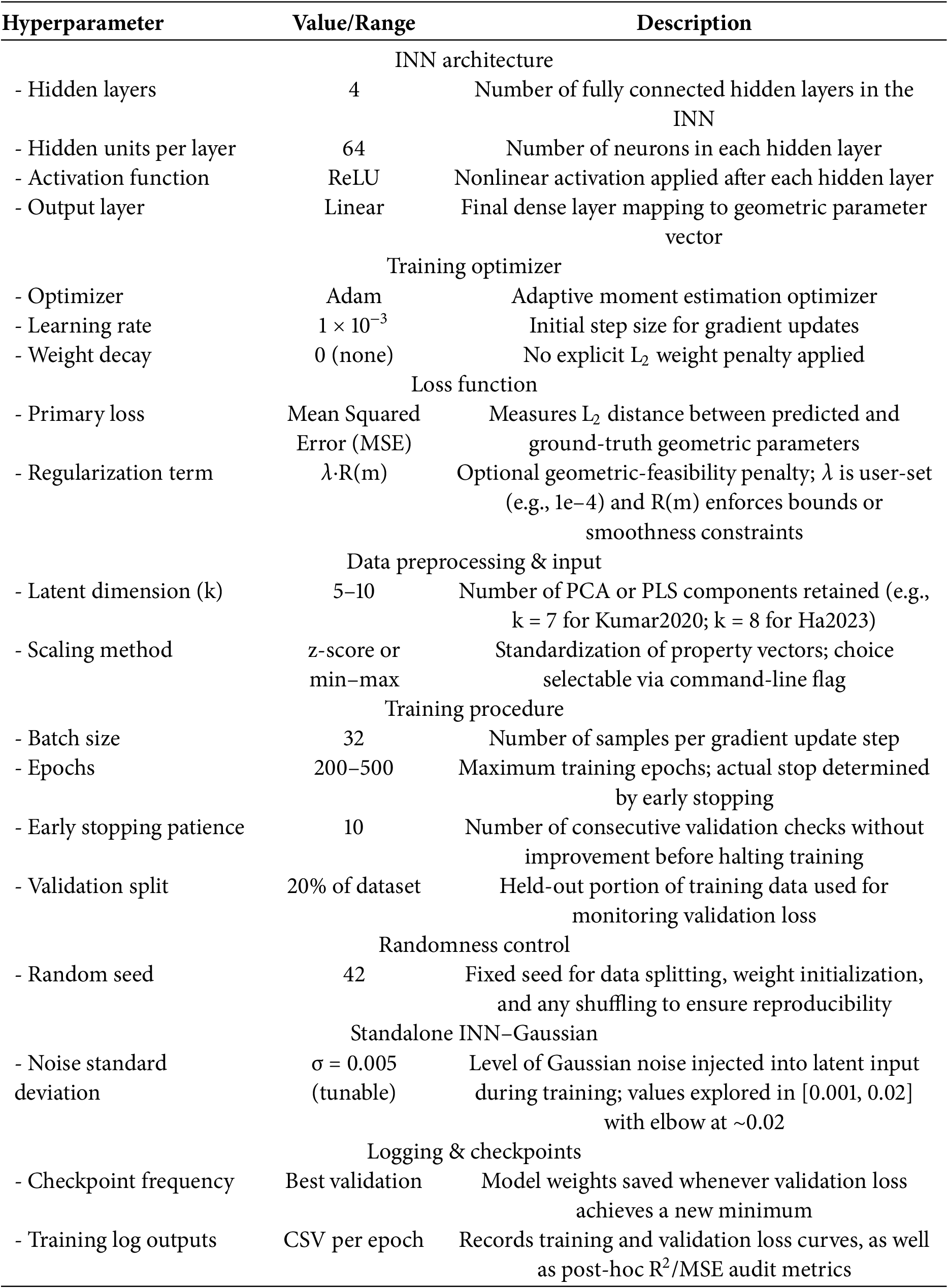
Appendix F Evaluation Procedure & Metrics
In addition to the description in Section 4 of the main text, the following supplementary details ensure full reproducibility of all standalone INN experiments.
Appendix F.1 Evaluation Metrics
After training, the standalone INN predicts geometric parameters for the held-out test split. These parameters are passed through a pretrained forward network (FNN) solely for audit. The following metrics are reported:
• Model Score: R2 between INN-predicted geometry and ground-truth geometry.
• Reconstruction Score: R2 and MSE between FNN-reconstructed properties and original target properties.
• Robustness Test: Gaussian noise (σ = 0.005) injected into latent inputs during inference; resulting variation in Reconstruction Score is recorded.
Appendix F.2 Summary of Results on Test Splits
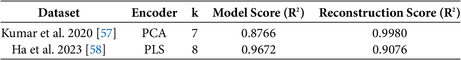
References
1. Edwards KL. Materials and design: the art and science of material selection in product design. Mater Des. 2003;24(5):401–2. doi:10.1016/s0261-3069(03)00043-8. [Google Scholar] [CrossRef]
2. Ashby MF, Shercliff H, Cebon D. Materials: engineering, science, processing and design. 4th ed. Oxford, UK: Butterworth-Heinemann; 2019. [Google Scholar]
3. Bhuvanesh Kumar M, Sathiya P. Methods and materials for additive manufacturing: a critical review on advancements and challenges. Thin Walled Struct. 2021;159:107228. doi:10.1016/j.tws.2020.107228. [Google Scholar] [CrossRef]
4. Bi Z, Wang X. Computer aided design and manufacturing. Hoboken, NJ, USA: John Wiley & Sons; 2020. [Google Scholar]
5. Huang CM, Kucinic A, Johnson JA, Su HJ, Castro CE. Integrated computer-aided engineering and design for DNA assemblies. Nat Mater. 2021;20(9):1264–71. doi:10.1038/s41563-021-00978-5. [Google Scholar] [PubMed] [CrossRef]
6. Top N, Şahin İ., Gökçe H, Gökçe H. Computer-aided design and additive manufacturing of bone scaffolds for tissue engineering: state of the art. J Mater Res. 2021;36(19):3725–45. doi:10.1557/s43578-021-00156-y. [Google Scholar] [CrossRef]
7. Choi JH, Kim H, Kim JY, Lim KH, Lee BC, Sim GD. Micro-cantilever bending tests for understanding size effect in gradient elasticity. Mater Des. 2022;214:110398. doi:10.1016/j.matdes.2022.110398. [Google Scholar] [CrossRef]
8. Manolis GD, Dineva PS, Rangelov T, Sfyris D. Mechanical models and numerical simulations in nanomechanics: a review across the scales. Eng Anal Bound Elem. 2021;128:149–70. doi:10.1016/j.enganabound.2021.04.004. [Google Scholar] [CrossRef]
9. Nasim M, Li Y, Wen M, Wen C. A review of high-strength nanolaminates and evaluation of their properties. J Mater Sci Technol. 2020;50:215–44. doi:10.1016/j.jmst.2020.03.011. [Google Scholar] [CrossRef]
10. Emovon I, Oghenenyerovwho OS. Application of MCDM method in material selection for optimal design: a review. Results Mater. 2020;7:100115. doi:10.1016/j.rinma.2020.100115. [Google Scholar] [CrossRef]
11. Farag MM. Materials and process selection for engineering design. Boca Raton, FL, USA: CRC Press; 2020. [Google Scholar]
12. Martins JR. Ning A. Engineering design optimization. New York, NY, USA: Cambridge University Press; 2021. [Google Scholar]
13. Abdolrasol MGM, Suhail Hussain SM, Ustun TS, Sarker MR, Hannan MA, Mohamed R, et al. Artificial neural networks based optimization techniques: a review. Electronics. 2021;10(21):2689. doi:10.3390/electronics10212689. [Google Scholar] [CrossRef]
14. Chen CT, Gu GX. Generative deep neural networks for inverse materials design using backpropagation and active learning. Adv Sci. 2020;7(5):1902607. doi:10.1002/advs.201902607. [Google Scholar] [PubMed] [CrossRef]
15. So S, Badloe T, Noh J, Bravo-Abad J, Rho J. Deep learning enabled inverse design in nanophotonics. Nanophotonics. 2020;9(5):1041–57. doi:10.1515/nanoph-2019-0474. [Google Scholar] [CrossRef]
16. Tan RK, Zhang NL, Ye W. A deep learning-based method for the design of microstructural materials. Struct Multidiscip Optim. 2020;61(4):1417–38. doi:10.1007/s00158-019-02424-2. [Google Scholar] [CrossRef]
17. Regenwetter L, Nobari AH, Ahmed F. Deep generative models in engineering design: a review. J Mech Des. 2022;144(7):071704. doi:10.1115/1.4053859. [Google Scholar] [CrossRef]
18. Liao X, Ma H, Tang YJ. Artificial intelligence: a solution to involution of design-build-test-learn cycle. Curr Opin Biotechnol. 2022;75:102712. doi:10.1016/j.copbio.2022.102712. [Google Scholar] [PubMed] [CrossRef]
19. Wang H, Fu T, Du Y, Gao W, Huang K, Liu Z, et al. Scientific discovery in the age of artificial intelligence. Nature. 2023;620(7972):47–60. doi:10.1038/s41586-023-06221-2. [Google Scholar] [PubMed] [CrossRef]
20. Dommaraju N, Bujny M, Menzel S, Olhofer M, Duddeck F. Evaluation of geometric similarity metrics for structural clusters generated using topology optimization. Appl Intell. 2023;53(1):904–29. doi:10.1007/s10489-022-03301-0. [Google Scholar] [CrossRef]
21. Xu Y, Tong X, Stilla U. Voxel-based representation of 3D point clouds: methods, applications, and its potential use in the construction industry. Autom Constr. 2021;126:103675. doi:10.1016/j.autcon.2021.103675. [Google Scholar] [CrossRef]
22. Kench S, Cooper SJ. Generating three-dimensional structures from a two-dimensional slice with generative adversarial network-based dimensionality expansion. Nat Mach Intell. 2021;3(4):299–305. doi:10.1038/s42256-021-00322-1. [Google Scholar] [CrossRef]
23. Bader C, Kolb D, Weaver JC, Sharma S, Hosny A, Costa J, et al. Making data matter: voxel printing for the digital fabrication of data across scales and domains. Sci Adv. 2018;4(5):eaas8652. doi:10.1126/sciadv.aas8652. [Google Scholar] [PubMed] [CrossRef]
24. Xu H, Dikin DA, Burkhart C, Chen W. Descriptor-based methodology for statistical characterization and 3D reconstruction of microstructural materials. Comput Mater Sci. 2014;85:206–16. doi:10.1016/j.commatsci.2013.12.046. [Google Scholar] [CrossRef]
25. Zou X, Lo SB, Sevilla R, Hassan O, Morgan K. The generation of tetrahedral meshes for NURBS-enhanced FEM. Eng Comput. 2024;40(6):3949–77. doi:10.1007/s00366-024-02004-z. [Google Scholar] [CrossRef]
26. Fu YF, Rolfe B, Chiu LNS, Wang Y, Huang X, Ghabraie K. Smooth topological design of 3D continuum structures using elemental volume fractions. Comput Struct. 2020;231:106213. doi:10.1016/j.compstruc.2020.106213. [Google Scholar] [CrossRef]
27. Nguyen-Van V, Li S, Liu J, Nguyen K, Tran P. Modelling of 3D concrete printing process: a perspective on material and structural simulations. Addit Manuf. 2023;61:103333. doi:10.1016/j.addma.2022.103333. [Google Scholar] [CrossRef]
28. Upadhyay BD, Sonigra SS, Daxini SD. Numerical analysis perspective in structural shape optimization: a review post 2000. Adv Eng Softw. 2021;155:102992. doi:10.1016/j.advengsoft.2021.102992. [Google Scholar] [CrossRef]
29. Bello SA, Yu S, Wang C, Adam JM, Li J. Review: deep learning on 3D point clouds. Remote Sens. 2020;12(11):1729. doi:10.3390/rs12111729. [Google Scholar] [CrossRef]
30. Han XF, Feng ZA, Sun SJ, Xiao GQ. 3D point cloud descriptors: state-of-the-art. Artif Intell Rev. 2023;56(10):12033–83. doi:10.1007/s10462-023-10486-4. [Google Scholar] [CrossRef]
31. Guo Y, Wang H, Hu Q, Liu H, Liu L, Bennamoun M. Deep learning for 3D point clouds: a survey. IEEE Trans Pattern Anal Mach Intell. 2021;43(12):4338–64. doi:10.1109/TPAMI.2020.3005434. [Google Scholar] [PubMed] [CrossRef]
32. Liu W, Sun J, Li W, Hu T, Wang P. Deep learning on point clouds and its application: a survey. Sensors. 2019;19(19):4188. doi:10.3390/s19194188. [Google Scholar] [PubMed] [CrossRef]
33. Tran TV, Nanthakumar SS, Zhuang X. Deep learning-based framework for the on-demand inverse design of metamaterials with arbitrary target band gap. npj Artif Intell. 2025;1:2. doi:10.1038/s44387-025-00001-1. [Google Scholar] [CrossRef]
34. Ulusoy U. A review of particle shape effects on material properties for various engineering applications: from macro to nanoscale. Minerals. 2023;13(1):91. doi:10.3390/min13010091. [Google Scholar] [CrossRef]
35. Veloso F, Gomes-Fonseca J, Morais P, Correia-Pinto J, Pinho ACM, Vilaça JL. Overview of methods and software for the design of functionally graded lattice structures. Adv Eng Mater. 2022;24(11):2200483. doi:10.1002/adem.202200483. [Google Scholar] [CrossRef]
36. Bishara D, Xie Y, Liu WK, Li S. A state-of-the-art review on machine learning-based multiscale modeling, simulation, homogenization and design of materials. Arch Comput Meth Eng. 2023;30(1):191–222. doi:10.1007/s11831-022-09795-8. [Google Scholar] [CrossRef]
37. Bostanabad R, Zhang Y, Li X, Kearney T, Brinson LC, Apley DW, et al. Computational microstructure characterization and reconstruction: review of the state-of-the-art techniques. Prog Mater Sci. 2018;95:1–41. doi:10.1016/j.pmatsci.2018.01.005. [Google Scholar] [CrossRef]
38. Hsu YC, Yu CH, Buehler MJ. Tuning mechanical properties in polycrystalline solids using a deep generative framework. Adv Eng Mater. 2021;23(4):2001339. doi:10.1002/adem.202001339. [Google Scholar] [CrossRef]
39. Sullivan J, Mirhashemi A, Lee J. Deep learning-based inverse design of microstructured materials for optical optimization and thermal radiation control. Sci Rep. 2023;13(1):7382. doi:10.1038/s41598-023-34332-3. [Google Scholar] [PubMed] [CrossRef]
40. Wang Q, Zhang L. Inverse design of glass structure with deep graph neural networks. Nat Commun. 2021;12(1):5359. doi:10.1038/s41467-021-25490-x. [Google Scholar] [PubMed] [CrossRef]
41. Batra R, Song L, Ramprasad R. Emerging materials intelligence ecosystems propelled by machine learning. Nat Rev Mater. 2021;6(8):655–78. doi:10.1038/s41578-020-00255-y. [Google Scholar] [CrossRef]
42. Cova TFGG, Pais AACC. Deep learning for deep chemistry: optimizing the prediction of chemical patterns. Front Chem. 2019;7:809. doi:10.3389/fchem.2019.00809. [Google Scholar] [PubMed] [CrossRef]
43. He L, Li Y, Torrent D, Zhuang X, Rabczuk T, Jin Y. Machine learning assisted intelligent design of meta structures: a review. Microstructures. 2023;3(4):2023034. doi:10.20517/microstructures.2023.29. [Google Scholar] [CrossRef]
44. Jin Y, He L, Wen Z, Mortazavi B, Guo H, Torrent D, et al. Intelligent on-demand design of phononic metamaterials. Nanophotonics. 2022;11(3):439–60. doi:10.1515/nanoph-2021-0639. [Google Scholar] [PubMed] [CrossRef]
45. Gebauer NWA, Gastegger M, Hessmann SSP, Müller KR, Schütt KT. Inverse design of 3D molecular structures with conditional generative neural networks. Nat Commun. 2022;13(1):973. doi:10.1038/s41467-022-28526-y. [Google Scholar] [PubMed] [CrossRef]
46. Zunger A. Inverse design in search of materials with target functionalities. Nat Rev Chem. 2018;2(4):121. doi:10.1038/s41570-018-0121. [Google Scholar] [CrossRef]
47. Chan TCY, Mahmood R, Zhu IY. Inverse optimization: theory and applications. Oper Res. 2025;73(2):1046–74. doi:10.1287/opre.2022.0382. [Google Scholar] [CrossRef]
48. Lininger A, Hinczewski M, Strangi G. General inverse design of layered thin-film materials with convolutional neural networks. ACS Photonics. 2021;8(12):3641–50. doi:10.1021/acsphotonics.1c01498. [Google Scholar] [CrossRef]
49. Mengu D, Rahman MSS, Luo Y, Li J, Kulce O, Ozcan A. At the intersection of optics and deep learning: statistical inference, computing, and inverse design. Adv Opt Photon. 2022;14(2):209–90. doi:10.1364/aop.450345. [Google Scholar] [CrossRef]
50. Ren Z, Tian SIP, Noh J, Oviedo F, Xing G, Li J, et al. An invertible crystallographic representation for general inverse design of inorganic crystals with targeted properties. Matter. 2022;5(1):314–35. doi:10.1016/j.matt.2021.11.032. [Google Scholar] [CrossRef]
51. Wang L, Chan YC, Ahmed F, Liu Z, Zhu P, Chen W. Deep generative modeling for mechanistic-based learning and design of metamaterial systems. Comput Meth Appl Mech Eng. 2020;372:113377. doi:10.1016/j.cma.2020.113377. [Google Scholar] [CrossRef]
52. Hou L, Jiao RJ. Data-informed inverse design by product usage information: a review, framework and outlook. J Intell Manuf. 2020;31(3):529–52. doi:10.1007/s10845-019-01463-2. [Google Scholar] [CrossRef]
53. Kumar Singh S, Rai R, Pradip Khawale R, Patel D, Bielecki D, Nguyen R, et al. Deep learning in computational design synthesis: a comprehensive review. J Comput Inf Sci Eng. 2024;24(4):040801. doi:10.1115/1.4064215. [Google Scholar] [CrossRef]
54. Ma W, Liu Z, Kudyshev ZA, Boltasseva A, Cai W, Liu Y. Deep learning for the design of photonic structures. Nat Photonics. 2021;15(2):77–90. doi:10.1038/s41566-020-0685-y. [Google Scholar] [CrossRef]
55. Alderete NA, Pathak N, Espinosa HD. Machine learning assisted design of shape-programmable 3D kirigami metamaterials. npj Comput Mater. 2022;8:191. doi:10.1038/s41524-022-00873-w. [Google Scholar] [CrossRef]
56. Bastek JH, Kumar S, Telgen B, Glaesener RN, Kochmann DM. Inverting the structure-property map of truss metamaterials by deep learning. Proc Natl Acad Sci U S A. 2022;119(1):e2111505119. doi:10.1073/pnas.2111505119. [Google Scholar] [PubMed] [CrossRef]
57. Kumar S, Tan S, Zheng L, Kochmann DM. Inverse-designed spinodoid metamaterials. npj Comput Mater. 2020;6:73. doi:10.1038/s41524-020-0341-6. [Google Scholar] [CrossRef]
58. Ha CS, Yao D, Xu Z, Liu C, Liu H, Elkins D, et al. Rapid inverse design of metamaterials based on prescribed mechanical behavior through machine learning. Nat Commun. 2023;14(1):5765. doi:10.1038/s41467-023-40854-1. [Google Scholar] [PubMed] [CrossRef]
59. Suganthan PN, Katuwal R. On the origins of randomization-based feedforward neural networks. Appl Soft Comput. 2021;105:107239. doi:10.1016/j.asoc.2021.107239. [Google Scholar] [CrossRef]
60. Borkowski L, Skinner T, Chattopadhyay A. Woven ceramic matrix composite surrogate model based on physics-informed recurrent neural network. Compos Struct. 2023;305:116455. doi:10.1016/j.compstruct.2022.116455. [Google Scholar] [CrossRef]
61. Cremonesi M, Franci A, Idelsohn S, Oñate E. A state of the art review of the particle finite element method (PFEM). Arch Comput Meth Eng. 2020;27(5):1709–35. doi:10.1007/s11831-020-09468-4. [Google Scholar] [CrossRef]
62. Paul S. Finite element analysis in fused deposition modeling research: a literature review. Measurement. 2021;178:109320. doi:10.1016/j.measurement.2021.109320. [Google Scholar] [CrossRef]
63. Richert C, Odermatt A, Huber N. Computation of thickness and mechanical properties of interconnected structures: accuracy, deviations, and approaches for correction. Front Mater. 2019;6:327. doi:10.3389/fmats.2019.00327. [Google Scholar] [CrossRef]
64. Zhuang Y, Chen W, Jin T, Chen B, Zhang H, Zhang W. A review of computer vision-based structural deformation monitoring in field environments. Sensors. 2022;22(10):3789. doi:10.3390/s22103789. [Google Scholar] [PubMed] [CrossRef]
65. Liu X, Tian S, Tao F, Yu W. A review of artificial neural networks in the constitutive modeling of composite materials. Compos Part B Eng. 2021;224:109152. doi:10.1016/j.compositesb.2021.109152. [Google Scholar] [CrossRef]
66. Chen Y, Lu L, Karniadakis GE, Negro LD. Physics-informed neural networks for inverse problems in nano-optics and metamaterials. Opt Express. 2020;28(8):11618–33. doi:10.1364/OE.384875. [Google Scholar] [PubMed] [CrossRef]
67. Yin W, Ge J, Meng P, Qu F. A neural network method for the inverse scattering problem of impenetrable cavities. Era. 2020;28(2):1123–42. doi:10.3934/era.2020062. [Google Scholar] [CrossRef]
68. Jiang J, Chen M, Fan JA. Deep neural networks for the evaluation and design of photonic devices. Nat Rev Mater. 2021;6(8):679–700. doi:10.1038/s41578-020-00260-1. [Google Scholar] [CrossRef]
69. Yao Z, Sánchez-Lengeling B, Bobbitt NS, Bucior BJ, Kumar SGH, Collins SP, et al. Inverse design of nanoporous crystalline reticular materials with deep generative models. Nat Mach Intell. 2021;3(1):76–86. doi:10.1038/s42256-020-00271-1. [Google Scholar] [CrossRef]
70. Zheng X, Zhang X, Chen TT, Watanabe I. Deep learning in mechanical metamaterials: from prediction and generation to inverse design. Adv Mater. 2023;35(45):e2302530. doi:10.1002/adma.202302530. [Google Scholar] [PubMed] [CrossRef]
Cite This Article
 Copyright © 2025 The Author(s). Published by Tech Science Press.
This work is licensed under a Creative Commons Attribution 4.0 International License , which permits unrestricted use, distribution, and reproduction in any medium, provided the original work is properly cited.
 Downloads
 Citation Tools