ELM-APDPs: An Explainable Ensemble Learning Method for Accurate Prediction of Druggable Proteins

1  Introduction

The human genome is made up of approximately 20,000 genes that encode proteins. However, it should be noted that not all proteins are viable targets for drug development [1–3]. The precise identification of therapeutic targets within the human body remains critical for the development of innovative pharmaceuticals. Compared to conventional experimental techniques, machine learning (ML)-based approaches have gained increasing attention due to their efficiency and predictive accuracy in drug-target identification tasks [4,5]. Recent advancements in explainable artificial intelligence have further strengthened ML-based models in biomedical applications, particularly for druggable protein prediction tasks [6]. A druggable protein is a protein that has the ability to strongly attach to tiny drug-like compounds and has beneficial therapeutic effects [7,8]. Druggable proteins typically belong to extensive protein families that have been effectively recognised as targets for drug development [9]. The primary cause of project failures in the field of drug development is commonly attributed to the undruggable nature of the target, as indicated by an estimated 60% of all cases [10]. Thus, the druggability of a protein plays a critical role in the advancement of a drug development initiative, as it is imperative to identify drug targets [11] accurately.

Computational techniques that rely exclusively on the primary sequences of pharmaceuticals have the potential to enhance experimental approaches by accelerating the process of characterizing and predicting proteins that are amenable to drug development. This urgency is amplified due to the extensive production of new proteins by next-generation sequencing, which presents a significant opportunity to uncover potential druggable proteins that have not yet been described [12]. Conventional experimental techniques can accurately detect the drug targets; however, these techniques are time-consuming and difficult for applications on a large scale [13]. For instance, the investigation of the three-dimensional structure of a protein is a necessary component of experimental procedures, leading to a protracted development cycle [14]. In contrast, computational methods that depend exclusively on pharmaceutical primary sequences can complement experiments to prioritize candidates efficiently [15].

Recent studies emphasize key criteria for optimal drug targets. Gashaw et al. note that an optimal drug target must possess selective expression in anatomical regions, minimal physiological impact, and compatibility with high-throughput screening [16,17]. Similarly, tools like DoGSiteScorer identify druggable binding pockets using geometric and physicochemical features [18], while sequence-based ML models like DrugMiner and DrugFinder [19], XGB-DrugPred [20], and others leverage amino acid composition for predictions [21,22]. Despite progress, fewer than 20% of the ~3000 proteins in the druggable genome are targeted by FDA-approved drugs [23], underscoring the need for improved frameworks.

Our hypothesis posits that the WDR protein family contains a greater number of druggable members [24–26]. We aimed to investigate this hypothesis within the framework of Target 2035, a worldwide endeavor to create pharmacological interventions for every human protein to address scalability. We focus on DEL-ML, a method overcoming practical limitations of DNA-encoded library screening [27,28]. We evaluate three feature extraction strategies: Dipeptide Deviation from Expected Mean (DDE), Enhanced Amino Acid Composition (EAAC), and Enhanced Grouped Amino Acid Composition (EGAAC) to identify optimal sequence descriptors for druggability prediction.

EGAAC, a feature extraction method grouping amino acids by physicochemical properties (e.g., hydrophobicity, charge), outperformed other techniques in capturing critical biochemical patterns for druggability prediction. Our approach employs ensemble learning, a technique combining multiple base models to enhance prediction accuracy. For example, the Gradient Boosting, Extreme Gradient Boosting, and Cat Boosting models achieved accuracies up to 68.33%, while Extreme Gradient Boosting Machine (XGBM) and Stacking models yielded 71.66% accuracy in dataset 1. These results demonstrate that ensemble methods outperform single classifiers, with EGAAC-based models showing superior performance.

We introduce CEL-IDP (Comparison of Ensemble Learning Methods for Identification of Druggable Proteins), a computational framework integrating amino acid composition features with stacking, boosting, and bagging strategies. By leveraging sequence-derived descriptors from protein primary structures, CEL-IDP captures informative biochemical patterns to prioritize druggable targets [29,30]. This work advances machine learning-driven drug discovery by systematizing ensemble learning for high-throughput druggability prediction, addressing the need for scalable methods to analyze large protein datasets, prioritizing the understudied WDR family, and contributing toward global efforts like Target 2035 [31].

2  Methods

2.1 Benchmark Druggable Protein Dataset (Evidence)

The benchmark dataset typically comprises positive samples (proteins capable of interacting with drugs) and negative samples (proteins incapable of interacting with drugs). We used Jamali et al.’s dataset [32]. To ensure a reliable comparison with current approaches. The 1611 druggable proteins have been obtained by using the Drug-Bank database, as previously reported. Similar sequences of these proteins, with respect to characteristics and composition, were eliminated using the Cluster Database at High Identity with Tolerance (CD-HIT) tool. Additionally, there are 1224 druggable proteins in the final set of positive samples. Likewise, the negative sample set was created by integrating the datasets presented by Bakheet and Doig [33]. First, the Swiss-Prot repository was used to obtain these sequences. Following the elimination of analogous sequences, 1300 non-druggable proteins persisted. The final benchmark dataset, which consists of 1218 druggable proteins, is employed in experimental data points amounting to 2518 druggable proteins, as shown in Table 1.

2.2 Feature Extraction Using Dipeptide Deviation from Expected Mean (DDE)

The normalization method is implemented on the data of each DDE vector feature profile, which comprises 400 elements. For the 400 vector characteristics extracted from the original protein profiles, the DDE model demonstrates the generation of score matrix functions. The initial step involves synchronizing all values with a common amino value. The frequency of amino acids is subsequently divided by the length of the sequence. In conclusion, formula X is used to scale all functional values. Means and standard deviations are derived using vector score feature profiles, which consist of 400 vector features. The DDE and 2D techniques are used to configure all vector profiles. The dipeptide composition, as described by Bhasin and Raghava (2004) [34], has been employed to forecast various protein sequence functions, as demonstrated by Dhanda et al. (2013) [35].

Hence, the Dipeptide Deviation from Expected Mean (DDE) method, developed by Saravanan and Gautham (2015) [36], Quantifies deviations in dipeptide frequencies within protein sequences to different enzymes from non-enzymes. The DDE function vector is derived using three parameters: (1) Observed dipeptide composition (Dc), (2) theoretical mean (TM), and (3) theoretical variance (Tv).

De(i)=niN(1)

Here, De(i) represents the observed frequency of a dipeptide i in the sequence, where ni is the number of occurrences of the dipeptide i, and N=L−1 is the total number of dipeptides in a sequence of length L.

TM(i)=Ci1CN×Ci2CN(2)

The theoretical mean (TM(i)) estimates the expected frequency of a dipeptide i, assuming independence between amino acids. Ci1 and Ci2 denote the counts of the first and second amino acid in dipeptide i across the entire dataset, while CN=61 represents the total codons (excluding three stop codons).

Tv(i)=TM(i)(1−TM(i))N(3)

The theoretical variance (Tv(i)) quantifies the expected variability of a dipeptide’s i frequency under the independence assumption, where N is the total dipeptides in the sequence.

DDE(i)=Dc(i)−TM(i)TV(i)(4)

The DDE score standardizes the deviation of observed dipeptide frequencies from their theoretical expectations, with higher absolute values indicating stronger deviations. A 400-dimensional feature vector is generated by computing DDE(i) for all 400 possible dipeptides.

DDEp={DDE(i),...,…DDE(n)},where,i=1,2,…,400(5)

2.3 Feature Extraction Using Enhanced Amino Acid Composition (EAAC)

The approach proposed according to Chen et al. [37] involves the extraction of sequential protein information, which is subsequently used to derive amino-acid frequency information.

g(m,n)=H(m,n)H(n),m∈{A,C,D,…,Y},n∈{W1,W2,....WL}(6)

This method calculated the frequency of amino acid m within sliding windows of the sequence. Denotes the count of amino acid m in the n-th window, and H(n) is the window length. For example, a window size of 5 residues is slid across the sequence to capture local compositional biases.

2.4 Enhanced Grouped Amino Acid Composition (EGAAC)

The computation of EGAAC is derived from the categorization of amino acids. This study classifies amino acids into five distinct categories based on their physicochemical characteristics [38]. This method uses protein sequences to create numerical feature vectors, which are derived from their respective properties. Amino acid are grouped into five categories based on psychochemical properties: aliphatic (such as G, A, V, L, M, I), aromatic (F, Y, W), positively charged (K, R, H), negatively charged (D, E), and neutral (S, T, C, P, N, Q). While here (H(g,n)) is the count of amino acids in group g within the n-th window, and H(n) is the window length, for example, 5 residues. This feature extraction approach is highly effective in bioinformatics research fields, particularly in the prediction of druggable proteins. The calculation of EGAAC is determined by the following equation:

EGAAC(g,n)=H(g,n)H(n),g∈{g1,g2,g3,g4,g5},n∈{W1,W2,....WL}(7)

2.5 Proposed Method Step by Step

Consequently, it is crucial to translate knowledge about protein sequences into numerical values that ensemble learning algorithms can comprehend and use [39–41]. This study utilized three methods for extracting characteristics from protein sequences. The three methods are.

The DDE, EGAAC, and EAAC. An approach to machine learning known as ensemble learning involves training many models. Commonly referred to as “weak learners,” they address the same problems and then combine them to achieve improved outcomes. By combining weak models, we can achieve a more precise model. The concept of Ensemble Learning encompasses three distinct models, including Bagging, Boosting, and Stacking. The fundamental framework comprises multiple machine learning models. The methodology known as CEL-IDPs Fig. 1 comprises five fundamental steps: (i) The researchers gathered datasets and benchmarking data, followed by preprocessing and eliminating redundant similarity, duplication deletion. (ii) Features were extracted to cover various characteristics of sequencing data. (iii) A feature representation learning methodology was utilized, and analysis was conducted using the t-distributed Stochastic Neighbor Embedding (t-SNE) algorithm. (iv) A predictor was constructed using a three-step distinct model: Bagging, Boosting, and Stacking. (v) The final classification model was constructed, as depicted in Fig. 1. The following sections have presented a comprehensive elucidation of each of these noteworthy phases.

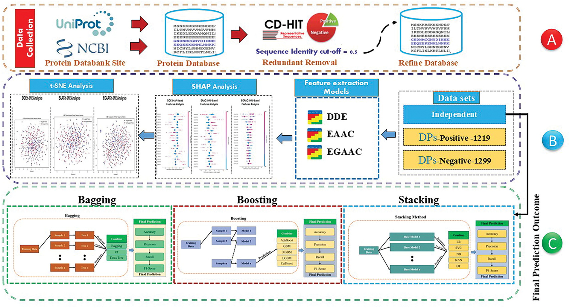
Figure 1: Workflow of the CEL-IDPs framework integrating feature extraction and ensemble learning for druggable protein prediction

Fig. 1 illustrates the proposed methodology’s comprehensive flow chart that depicts the organized process of our proposed methodology for identifying druggable proteins. In Section A, we compiled and improved a dataset of both druggable and non-druggable proteins, assuring data quality through redundancy. Section B emphasizes feature analysis, wherein we do SHAP analysis to elucidate feature significance, followed by t-SNE for data visualization. Furthermore, we obtained essential protein sequence descriptors, namely DDE, EAAC, and CGAAC. Section C delineates the predictive modeling phase in which various ensemble learning techniques-bagging, boosting, and stacking were employed to improve model generalizability and classification efficacy. The initial phase was the construction of a database containing both druggable and non-druggable proteins. Subsequently, the calculation of three families of protein composition descriptors was performed using Python. These descriptors included the 20 amino acid composition (AC), the Dipeptide deviation from expected mean (DDE), features length was 400, the Enhanced amino acid composition (EAAC) method, features length was 920, and the enhanced grouped amino acid composition (EGAAC) method, features length was 230. In the subsequent phase, Jupyter notebooks were utilized to implement Python/Scikit-learn-based machine learning classifiers [42]. These classifiers were constructed by integrating thirteen distinct types, which were derived from the combination of three descriptor families (DDE, EAAC, EGAAC). The classifiers utilized in this study encompassed a range of machine learning algorithms. First step, we conducted all analyses using the Bagging method first (Bagging Classifier) [43], second, the random forest (Random Forest Classifier) [44], and third, the decision tree (Decision Tree Classifier) [45]. In the second step, we used quantitative techniques to analyze the Boosting method, specifically, first AdaBoost [45], GB Boost [46], XGBM [47], LGBM, and CatBoost classifiers are used for the prediction of DPs sites. In the third step, we used the stacking method to combine quantitative techniques for analysis, which was based on first LR, SVC, NB [48], KNN [49], and DT [50] classifiers for the prediction of DPs sites. XGBoost (XGB) is an alternative ensemble method that utilizes sequential weak trees to rectify classification errors [47]. Using gradient boosting to classify is a well-established bootstrapping technique that relies on utilizing a succession of consecutive weak classifiers. A meta-estimator called the Ada-Boost classifier (AdaBoost) [45] starts the fitting process using a classifier that was created from the original dataset. Subsequently, it incorporates many iterations pertaining to the initial classifier, each with modified weights to account for cases that were improperly categorized. The Bagging classifier, also known as Bagging, shares similarities with AdaBoost. In Bagging, supplementary classifiers are produced from sub-sets of the initial dataset. The prediction model for machine learning was developed with distinct protein datasets. The positive set comprised 1219 druggable proteins, identified through their inclusion in the DrugBank database (www.drugbank.ca) and their correlation with FDA-approved pharmaceuticals. Conversely, the negative protein collection consisted of 1299 proteins that are not amenable to pharmacological targeting, as reported in a previous study.

The final machine learning prediction model was used to analyze three sets of cancer-associated protein lists. A total of 230 proteins were identified as essential in the BC dataset [51]. Additionally, 2353 proteins known to drive cancer were obtained from the Network of Cancer Genes [52], while 1365 proteins were classified as RNA-binding proteins (RBPs).

2.5.1 Bagging Method

In this analysis, bagging is a popular ensemble learning technique that combines the predictive outcomes of various base classifiers to provide a robust final classification result. The integration technique involves acquiring training subsets by selecting from the initial dataset, with each subset used to train a distinct model. The classification outcomes of samples are derived by a voting approach. As shown in Fig. 2.

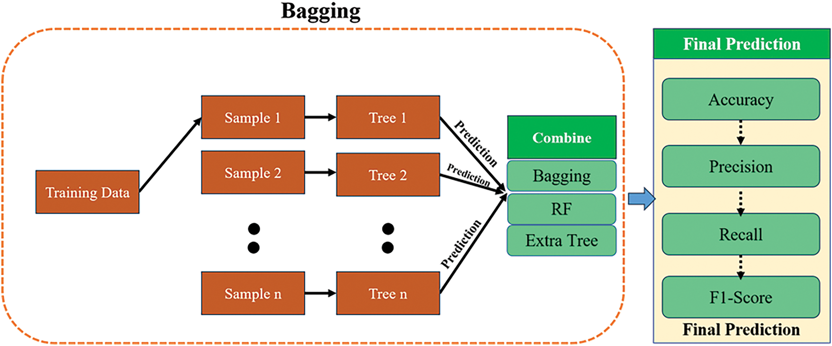
Figure 2: The bagging model framework combines three classifiers

1.    Bagging

2.    Random Forest algorithm

3.    Extra Trees

The Decision Tree model was chosen as the base model due to its consistent and outstanding performance in prior research studies [53–55].

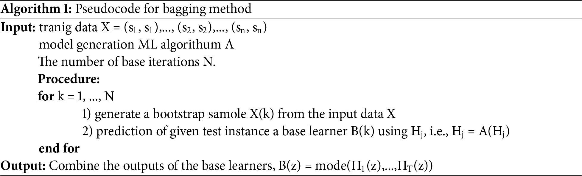
Bagging is a method that employs random sampling to divide the training data related to every base learner into subsets for training. The fundamental learners are aggregated through majority voting to form a robust classifier. The bagging method employed is detailed in Algorithm 1. The most prevalent example of bagging implementations is random forests.

2.5.2 Boosting Method

Boosting is a machine learning technique that combines adaptive sequential learning with a single base model. The optimal outcomes are obtained by combining the outcomes of each basis model with the outcomes of the preceding base model, as seen in Fig. 3.

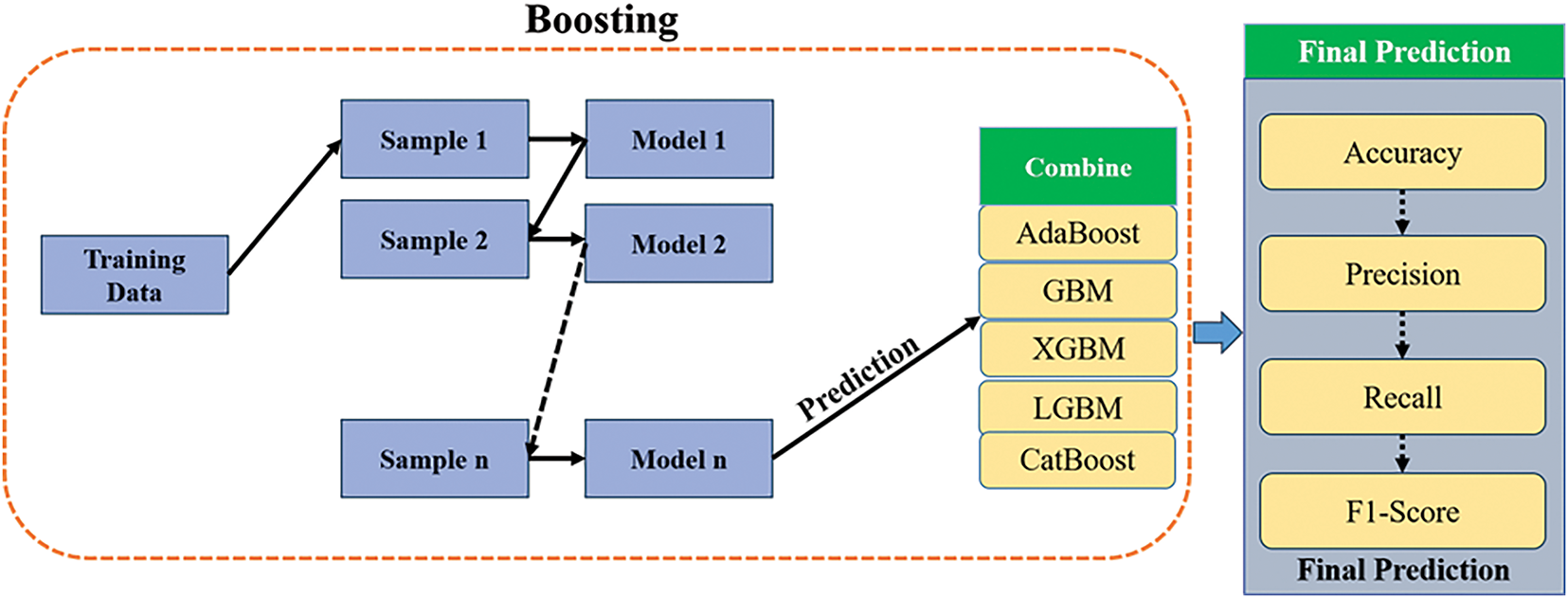
Figure 3: The boosting model framework combines five classifiers

The AdaBoost model, also known as Adaptive Boosting, was chosen to improve ensemble learning.

1.    The acronym GBM refers to Gradient Boosting Machines.

2.    Extra Gradient Boosting Machine (XGBM)

3.    The Light Gradient Boosting Machine (LGBM) algorithms.

4.    CatBoost is the fifth choice.

The Decision Tree model was chosen as the base model because it consistently produced excellent results in earlier research [53–55].

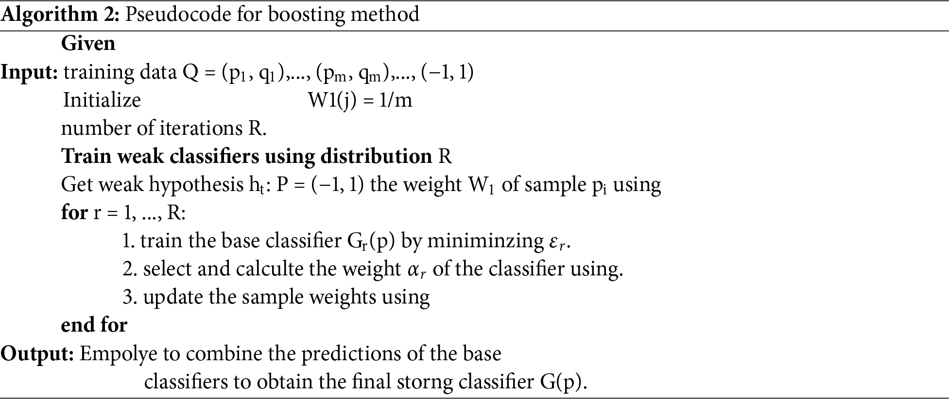
Using decision trees as base learners with a single split, AdaBoost is the first and most successful boosting method. The best way to use AdaBoost, which is used for binary classification tasks, is with AdaBoost M1. The Algorithm 2 explains the boosting method.

2.5.3 Stacking Method

Stacking is a method in Ensemble Learning wherein many base models are trained independently and simultaneously. The basic models are subsequently integrated through a meta-learning method to obtain the ultimate output, which is derived from the amalgamation of their respective findings. The design of the stacking model consists of many base models, termed level-0 models, in conjunction with a meta model that integrates the predictions of the base models, identified as a level-1 model, as illustrated in Fig. 4. The stacking ensemble learning experiment will utilize five base models, specifically:

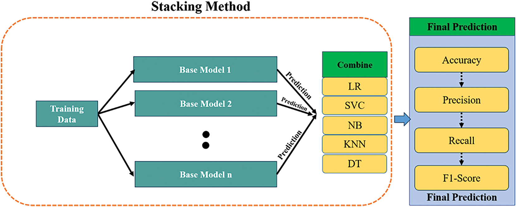
Figure 4: The stacking model architecture includes five classifiers

1.    Logistic Regression

2.    Support Vector Machine (SVC)

3.    Gaussian Naive Bayes

4.    K-Nearest Neighbor algorithm

5.    Decision Trees

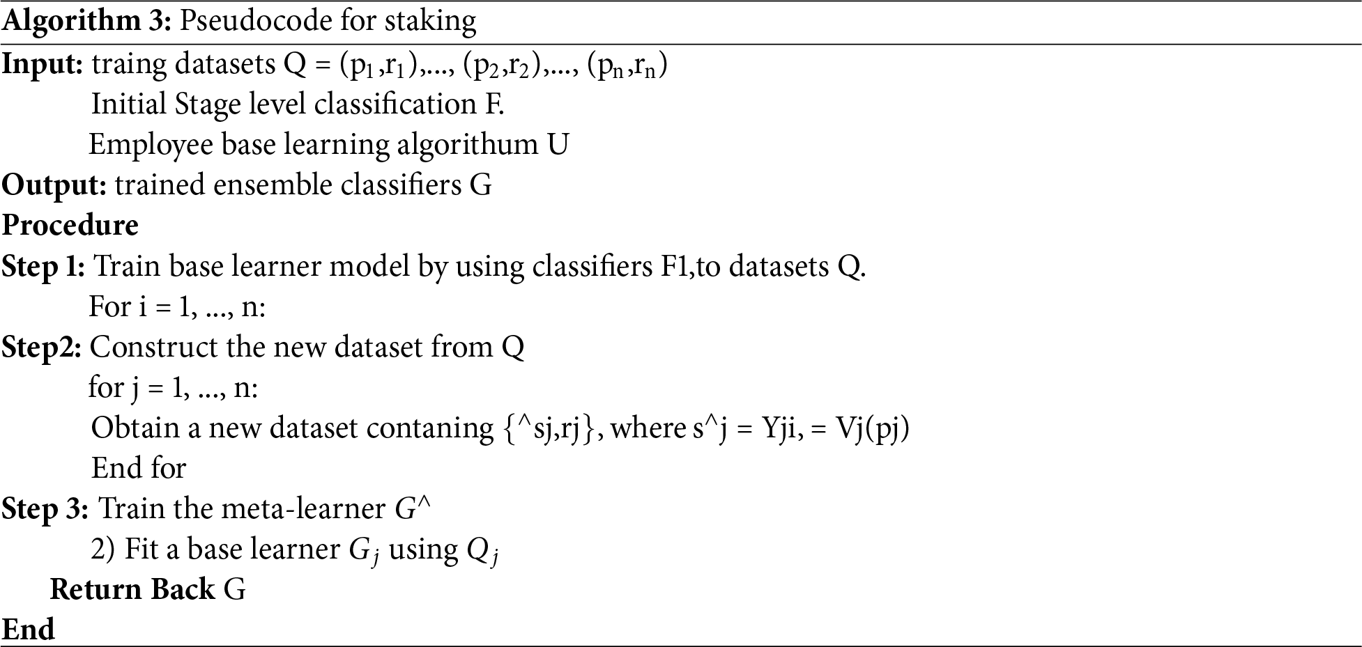
Logistic regression has been selected as the meta-model, while the stacking procedure is described in Algorithm 3.

The ML classifiers were constructed using a 5-fold cross-validation (CV) technique. A pipeline was established for every fold in the experiment. The test set was scaled to correspond with the same scale after the training set was scaled utilizing the Standard Scaler. The AUROC scores for these three ensemble learning methods in all splits were calculated using a cross-validation score. The mean values and standard deviation (SD) of the area under the receiver operating characteristic curve (AUROC) were reported for each machine learning classifier on the test subset. Following the utilization of a machine learning model to screen three protein sets associated with cancer, the proteins deemed suitable for drug targeting were subjected to analysis using g: Profiler (https://biit.cs.ut.ee/gprofiler/, accessed on 01 January 2025). This research aimed to deliver significant annotations (with a false discovery rate under 0.001) pertaining to gene ontology (GO) concepts, pathways, and disease phenotypes [39]. Circos plots were generated to visually represent the current status of clinical trials associated with the most potential druggable proteins identified by the Open Targets Platform (https://www.targetvalidation.org). The platform in question is a thorough data integration system that makes it easier to obtain and visualize potential targets for cancer treatment [40].

3  Model Performance Evaluation

Each model undergoes assessment through the metrics of Accuracy, Precision, and Recall. The values derived from the confusion matrix, which comprises true positive (TP), true negative (TN), false positive (FP), and false negative (FN) values, are used to compute these three measures. The computation of accuracy entails dividing the aggregate of true positives and true negatives by the overall data volume. It provides a comprehensive analysis of the outcomes achieved using the recommended methodology. The proposed technique is assessed in comparison with current methods to demonstrate its superior performance. The PR curves and the AUPRC are more informative regarding performance in class-imbalanced cases than the ROC curves in isolation. To add the PR curves and AUPRC scores to our performance evaluation. We added graphical PR-curves for the proposed and baseline methods in the revised manuscript, along with a paragraph underlining their importance in the presence of unbalanced data (Please see revised Section 4.10). These findings further support the robustness of our method in recognizing druggable proteins, especially when it comes to imbalanced classes.

Accuray=TP+TnTp+Tn+Fp+Fn(8)

Precision=TPTp+Fp(9)

Recall=TPTp+Fn(10)

F1-Score=2×Precision×recallPrecision+recall(11)

4  Results and Discussion

The project aims to propose novel classification models for the prediction of newly druggable proteins. This will be achieved by utilizing three families of protein composition descriptors, namely DDE, EAAC, and EGAAC, which are derived using the ensemble learning methods. Jupyter notebooks, utilizing Python and the sklearn library, were employed to construct classifiers employing a total of thirteen distinct machine learning classifiers and five distinct feature selection approaches. Various parameters were employed in this process, as depicted in Fig. 1. The categorization performance was quantified using AUROC in the scripts. We conducted experiments using models that had varying numbers of features, specifically 400, 920, and 230, as well as models with a combination of different feature quantities. The AUROC values provided in this study are the mean values obtained after a five-fold cross-validation process.

4.1 Ensemble Learning Methods for Accuracy Comparison Results

In Table 2, the results of our study indicate a requirement for improved outcomes in order to demonstrate that the proposed methodologies of bagging, boosting, and stacking improve the performance of these three feature extraction methods. DDE, EAAC, and EGAAC approaches. Results were considered significant. DDE features were used with bagging (RF obtained 66.87%), boosting (XGBM obtained 66.66%), and stacking (Stacking obtained a score of 68.33%). After that, EAAC features used bagging (Bagging obtained 66.66%), boosting (CatBoost obtained 56.66%), and stacking (Stacking obtained a score of 66.66%). Third EGAAC features were considered significant and outstanding, with bagging (RF obtained 71.66%), boosting (XGBM obtained 71.66%), and stacking (Stacking obtained a score of 68.33%). The highest level of performance is achieved by employing the EGAAC feature extraction method with bagging, boosting, and stacking methods.

4.2 Ensemble Learning Methods for DDE Features Performance Comparison Results

Results were considered significant. DDE features were used with bagging (RF obtained 66.87%), boosting (XGBM obtained 66.66%), and stacking (Stacking obtained a score of 68.66%), as shown in Table 3. The initial data set, referred to as the independent dataset, was created using the DDE model and the bagging, boosting, and stacking strategies. Table 3 illustrates this. The stacking method exhibits the greatest accuracy among ensemble learning techniques, attaining an accuracy score of 68.33%, as illustrated in Fig. 5. Additionally, the stacking process produces precise outcomes.

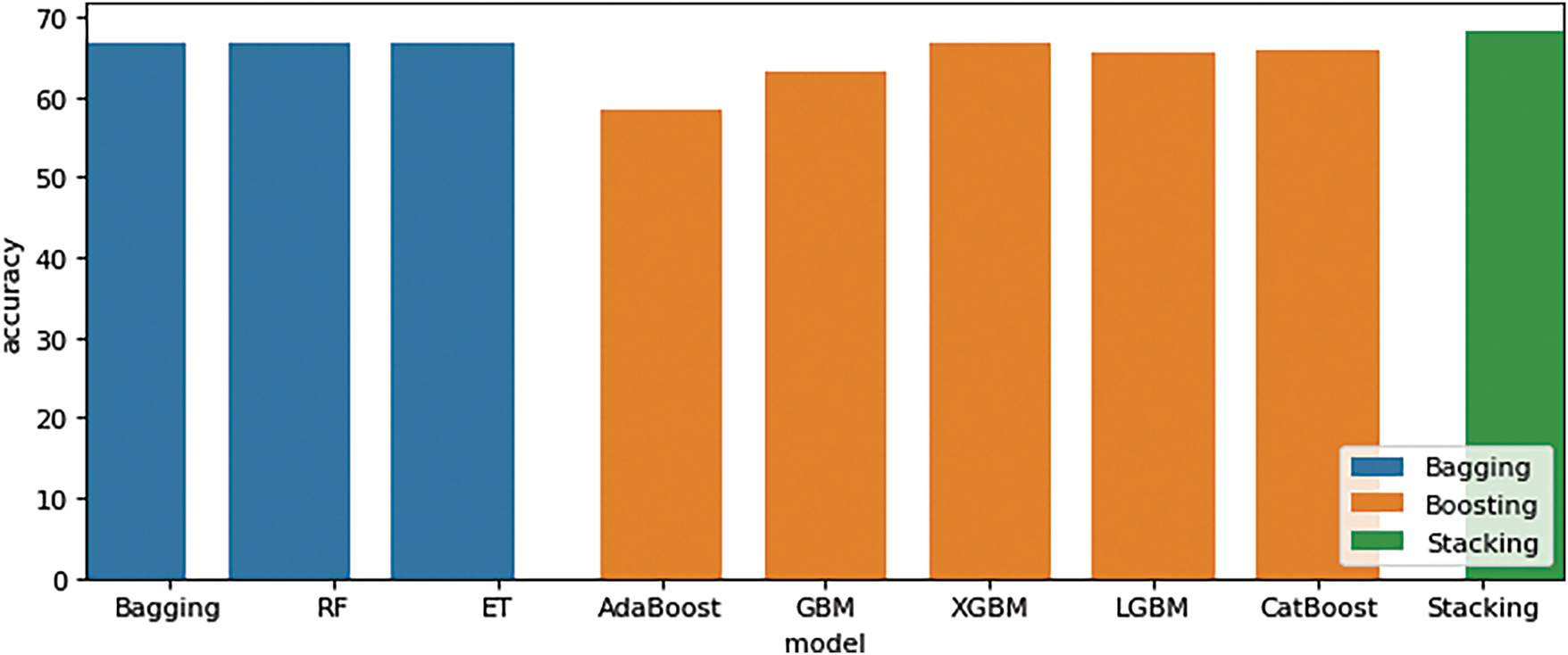
Figure 5: DDE features performance comparison results (Bagging, Boosting, and Stacking)

4.3 Ensemble Learning Methods for EAAC Features Performance Comparison Results

After that, EAAC features used bagging (Bagging obtained 66.66%), boosting (CatBoost obtained 56.66%), and stacking (Stacking obtained a score of 66.66%), as shown in Table 4. This is feasible due to the significantly larger amount of data in the dataset compared with dataset 1. It makes it possible for the model to enhance its learning efficiency, as illustrated in Fig. 6. Furthermore, it is possible that the data employed has a distinct pattern. According to the experimental results on the dataset, the boosting methods AdaBoost, XGB, and Light Gradient Boosting, as well as the random forest Bagging model, attained an average accuracy of 56.66%. Boosting has greater accuracy than bagging and stacking, as evidenced by the prior dataset, with the stacking method achieving the highest accuracy at 66.66%.

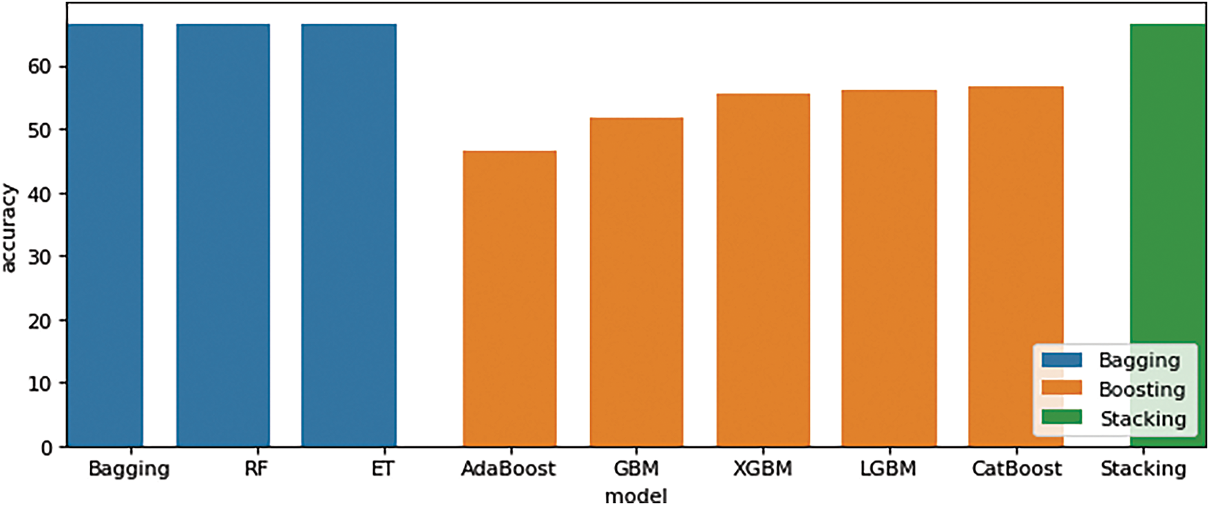
Figure 6: EAAC features performance comparison results (Bagging, Boosting, and Stacking)

4.4 Ensemble Learning Methods for EGAAC Features Performance Comparison Results

Third EGAAC features were considered significant and outstanding results with bagging (RF obtained 71.66%), boosting (XGBM obtained 71.66%), and stacking (Stacking obtained a score of 68.33%), as shown in Table 5. The highest level of performance is achieved by employing the EGAAC feature extraction method using bagging, boosting, and stacking techniques, as illustrated in Fig. 7. Table 5 displays the results of ensemble learning experiments performed on a separate dataset utilizing the EGAAC model. The accuracy acquired from the experimental findings of three ensemble learning approaches, specifically Bagging, Boosting, and Stacking, varied across three distinct datasets.

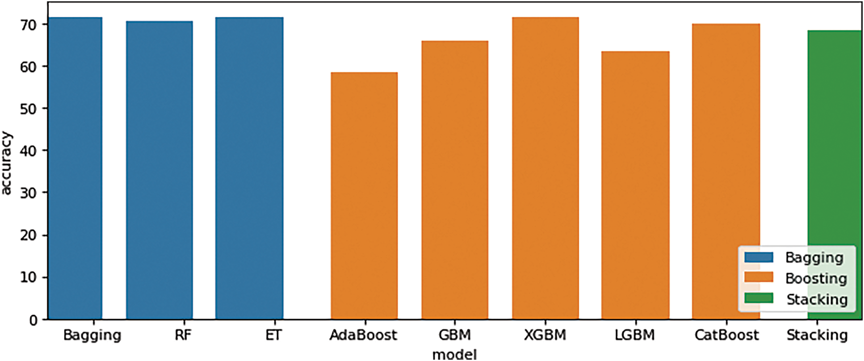
Figure 7: EGAAC features performance comparison results (Bagging, Boosting, and Stacking)

4.5 Comprehensive Evaluation and Interpretability of Classifiers

4.5.1 Classifier Performance Comparison

To evaluate the classification efficacy of various machine learning methods, as shown in Fig. 8, we analyzed the performance of many base classifiers and ensemble models employing common evaluation metrics: accuracy, precision, recall, F1-score, and ROC AUC. Table 6 summarizes the findings for nine classifiers: Random Forest, Gradient Boosting, Support Vector Machine (SVM), Logistic Regression, Decision Tree, Voting (both Hard and Soft), Bagging, and Stacking. The Stacking classifier exhibited the highest overall performance among all models, achieving an F1-score of 0.6683 and a ROC AUC of 0.7219. Subsequently, Soft Voting and Random Forest classifiers were thoroughly examined. These findings underscore the efficacy of ensemble learning methodologies in improving prediction accuracy and model resilience for the identification of druggable proteins.

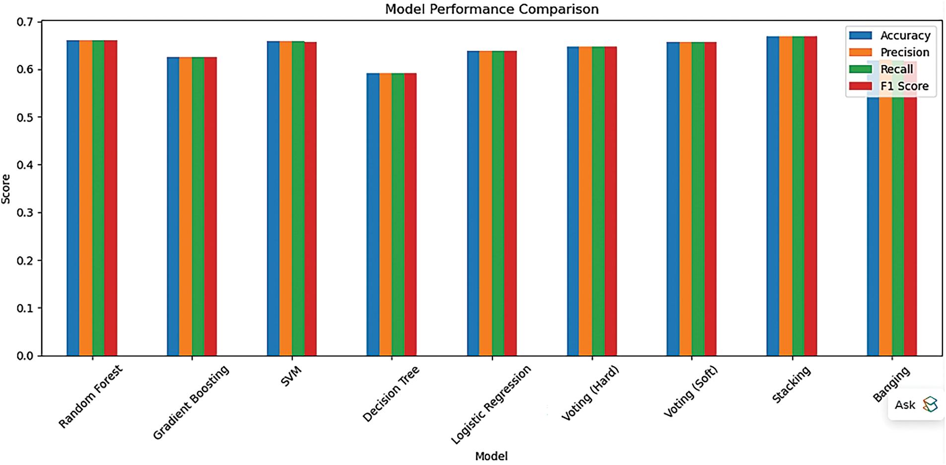
Figure 8: Visual comparison of classifier performance using evaluation metrics

4.5.2 Confusion Matrix Analysis

We visualized the confusion matrices for selected classifiers to conduct a more in-depth analysis of model performance. These matrices depict the quantities of true positives, true negatives, false positives, and false negatives, offering a comprehensive assessment of each model’s efficacy in differentiating between druggable and non-druggable proteins. Fig. 9 illustrates that the Stacking and Soft Voting classifiers yield the most equitable classification outcomes, exhibiting superior true positive and true negative rates relative to other models. These visual diagnostics validate the efficacy and generalizability of ensemble-based approaches in protein classification.

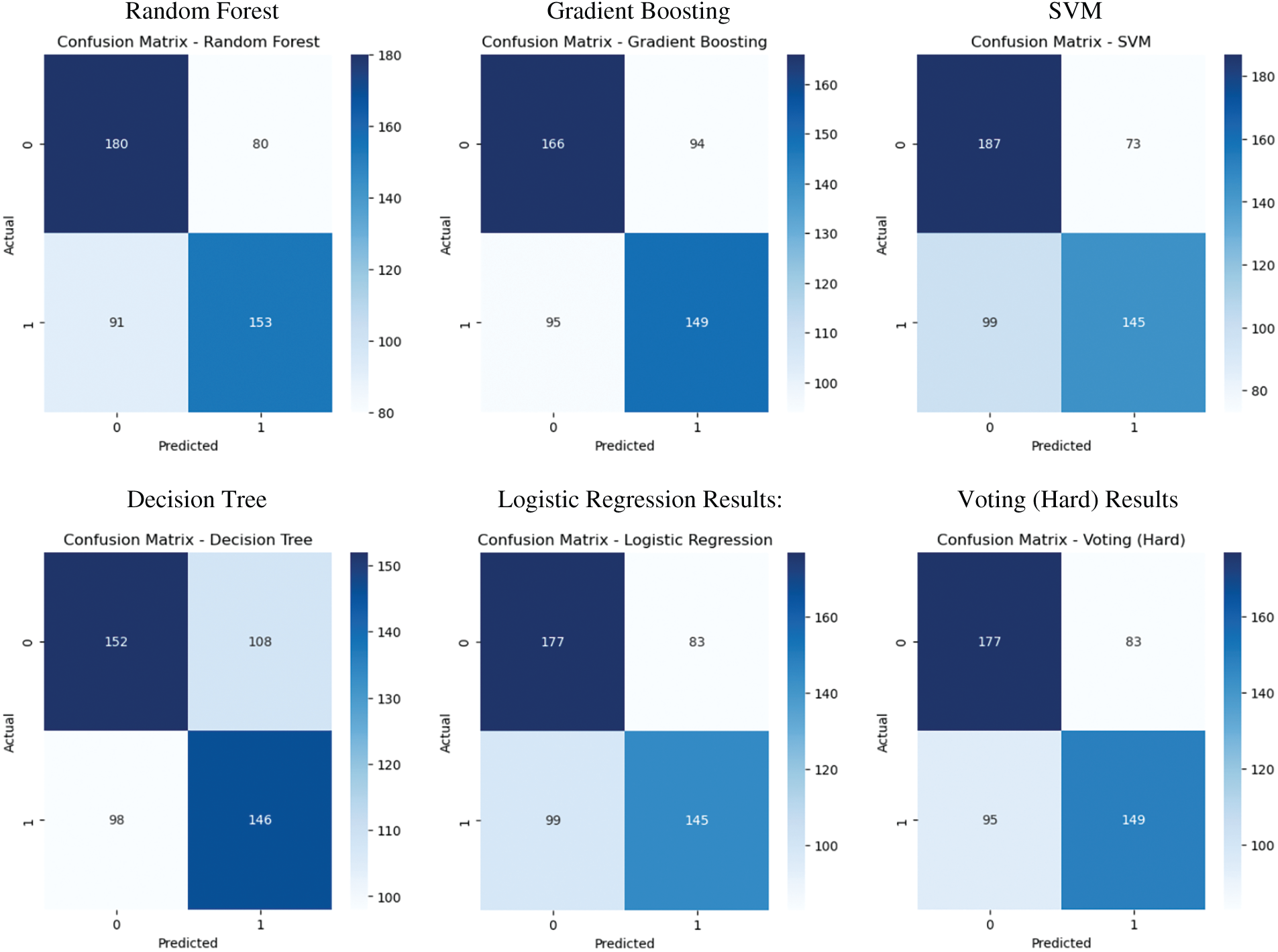
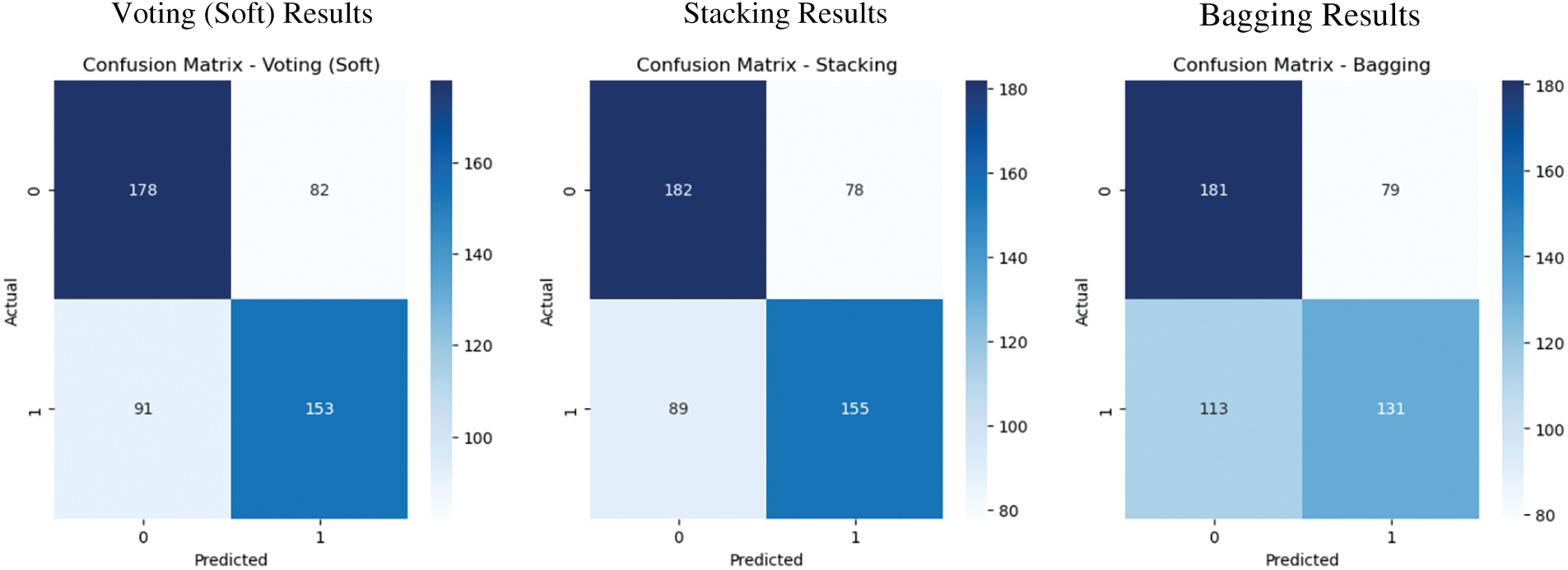
Figure 9: Confusion matrix visualizations for selected classifiers

4.5.3 Feature Importance from Random Forest

We evaluated feature relevance using the Random Forest model to determine which input features most significantly contributed to the classification process. Importance scores were derived using the Gini impurity criterion. As shown in Fig. 10, many of the top-ranked features originated from the EGAAC encoding method, highlighting the biochemical significance of amino acid classifications based on physicochemical groupings. These features substantially improved the model’s ability to distinguish between druggable and non-druggable proteins, offering critical insights into model interpretability and offering critical insights into model interpretability.

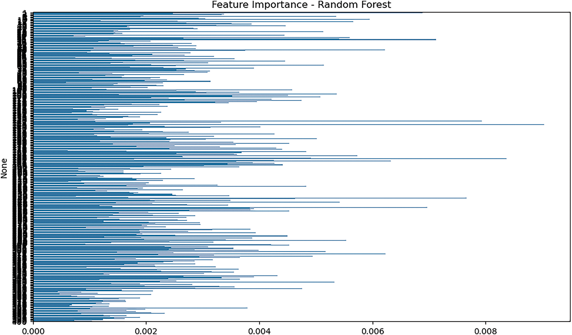
Figure 10: Feature importance plot from the random forest model

The magnitude levels of the attributes are plotted against the axis for the purposes of the discussion. The scores are computed based on the Gini impurity criterion and indicate the contribution of a feature in the classification process. A higher number indicates the characteristic is more important. Y-axis (Features): Each row represents one of the features from the dataset. The longer the line length, the more important this feature is in determining the category.

RHS: The features in contrast (RHS) have higher importance ratings, and they have a greater impact on the decision process of the machine. These features likely closely relate to the output class (eg, distinguishing between druggable and non-druggable proteins in your case). Left side features that are less significant and contribute little to the classification. Rightward extending features (which correspond to high importance) probably originated from the EGAAC encoding procedure, as discussed in the text. The physicochemical properties of the amino acid residues seem to heavily influence the prediction of druggability. Leftward features with shorter bars may be less important or may be redundant information for making precise predictions.

4.6 Comparative Analysis with Existing Druggable Proteins Prediction

Prioritizing previously identified genes based on the Pharmacogenomics Knowledgebase (PharmGKB), the interpreter for cancer genomes, and the Consensus Strategy of the Pan-Cancer Atlas project, we conducted comprehensive analyses of genetic changes, signaling pathways, protein interactions, networks, protein expression, dependency maps, and enrichment maps in a prior study. These investigations enabled us to identify critical proteins linked to the etiology of breast cancer. Predicting the draggability of breast cancer (BC) proteins using machine learning (ML) techniques has the potential to provide important information about potential biomarkers, potential treatment targets, and upcoming clinical trials. This strategy could improve precision medicine and global cancer pharmacogenomics while reducing ethnic bias [56,57].

4.7 SHAP-Based Feature Analysis for Druggable Protein Identification

To enhance the interpretability of our predictive model, we utilized SHAP (SHapley Additive exPlanations) to analyze the impact of specific characteristics in distinguishing druggable and non-druggable proteins. Unlike traditional feature selection methods, through the quantification of each feature’s influence on the model’s decision-making mechanism, SHAP offers a simple way to gauge the value of features [58].

Fig. 11 illustrates the SHAP-based feature analysis applied to three different feature encoding methods: Dipeptide Deviation Encoding (DDE), Enhanced Amino Acid Composition (EAAC), and Extended Grouped Amino Acid Composition (EGAAC). The SHAP plots reveal the most influential features contributing to the classification process. Features with high SHAP values strongly influence the model’s decision in favor of druggable proteins (positive impact) or non-druggable proteins (negative impact). These findings offer deeper insights into the biochemical properties that play a crucial role in druggability prediction, thereby strengthening the biological relevance of our model.

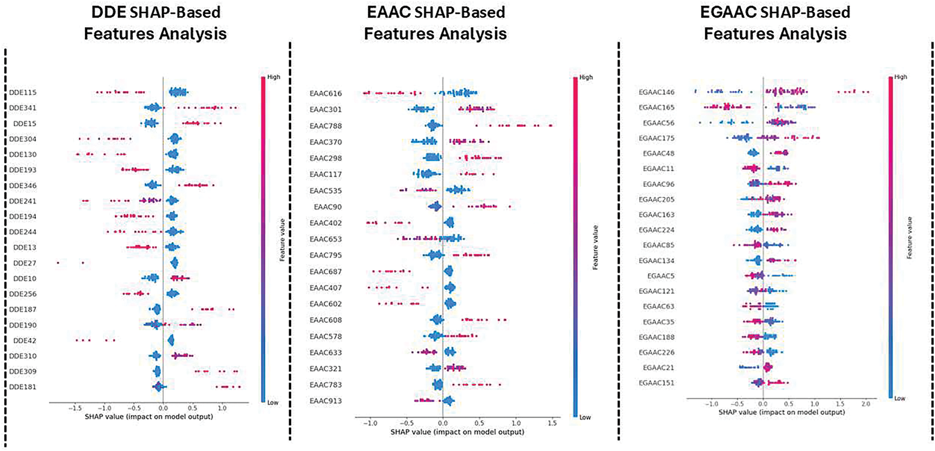
Figure 11: SHAP-based feature (Bagging, Boosting, and Stacking)

The figure demonstrates SHAP (SHapley Additive exPlanations)-based feature analysis applied to different datasets (DDE, EAAC, and EGAAC) using three different machine learning techniques: Bagging, Boosting, and Stacking. While SHAP values explain the importance of features for the model’s prediction, the figure does not make the relevant biology behind these traits as they relate to drug targets for identification, as you observed. Guided visualization and interpretation of SHAP-Inspired results: To improve the interpretability and utility of the SHAP-based research image shown in this study, it is important to annotate these top-ranked features (by the SHAP because these features are considered top-ranked features) with known biology and biological relationships. Conduct checks on the literature to ensure that these top-ranking features (e.g., “DDE115,” “EAAC616,” “EGAAC146,” etc.) actually correspond to biological functions or diseases that are relevant to the new drug target prediction. Explore whether these characteristics are linked to known biomarkers, genes, proteins, or pathways related to diseases such as cancer, diabetes, or neurodegenerative diseases. A functional relationship can be established if the features in the datasets are related to gene expression or protein activities; otherwise, use Gene Ontology (GO) analysis or pathway databases (e.g., KEGG, Reactome, or STRING). For example, one might question whether the genes linked to the affected traits are involved in specific biological processes like cell growth, death, or immunological response. Use bioinformatics techniques to determine if these features are similar to known functional domains, molecular functions, or biological processes. Often, highly maintainable features in biological datasets represent core regulatory proteins, enzymes, and receptors that are involved in drug-target interactions. Cross-reference resulting core traits with biological databases (e.g., UniProt, Ensembl, and/or GeneCards) to identify their implication in established pharmacological targets. This might provide strong support that these core characteristics may serve as potential targets for therapy. Once features are associated with biological pathways or molecular mechanisms, experimental validation such as CRISPR-based knockdown experiments or small molecules screen can validate the potentiality of the features as therapeutic targets. This approach, by linking SHAP-based features to biological literature, can contribute to a better understanding of their impact on drug discovery and possibly help identify new drug targets. It would also improve the interpretability of the SHAP study and bridge computational models with biological insights.

4.8 t-SNE Visualization of Feature Space

To further investigate the separability of druggable and non-druggable proteins in the learned feature space, the nonlinear dimensionality reduction method t-Distributed Stochastic Neighbor Embedding (t-SNE) was utilized [59]. Fig. 12 presents the t-SNE projections for the DDE, EAAC, and EGAAC feature encodings, providing a 2D visualization of the distribution of protein sequences. Each dot in the scatter plots represents a protein, with druggable proteins marked in blue and non-druggable proteins in red. The clustering patterns observed in the t-SNE plots suggest that different feature representations have varying degrees of discriminatory power. While some encodings exhibit better separation between druggable and non-druggable proteins, others display overlapping distributions, indicating that feature selection and fusion strategies may further improve classification performance.

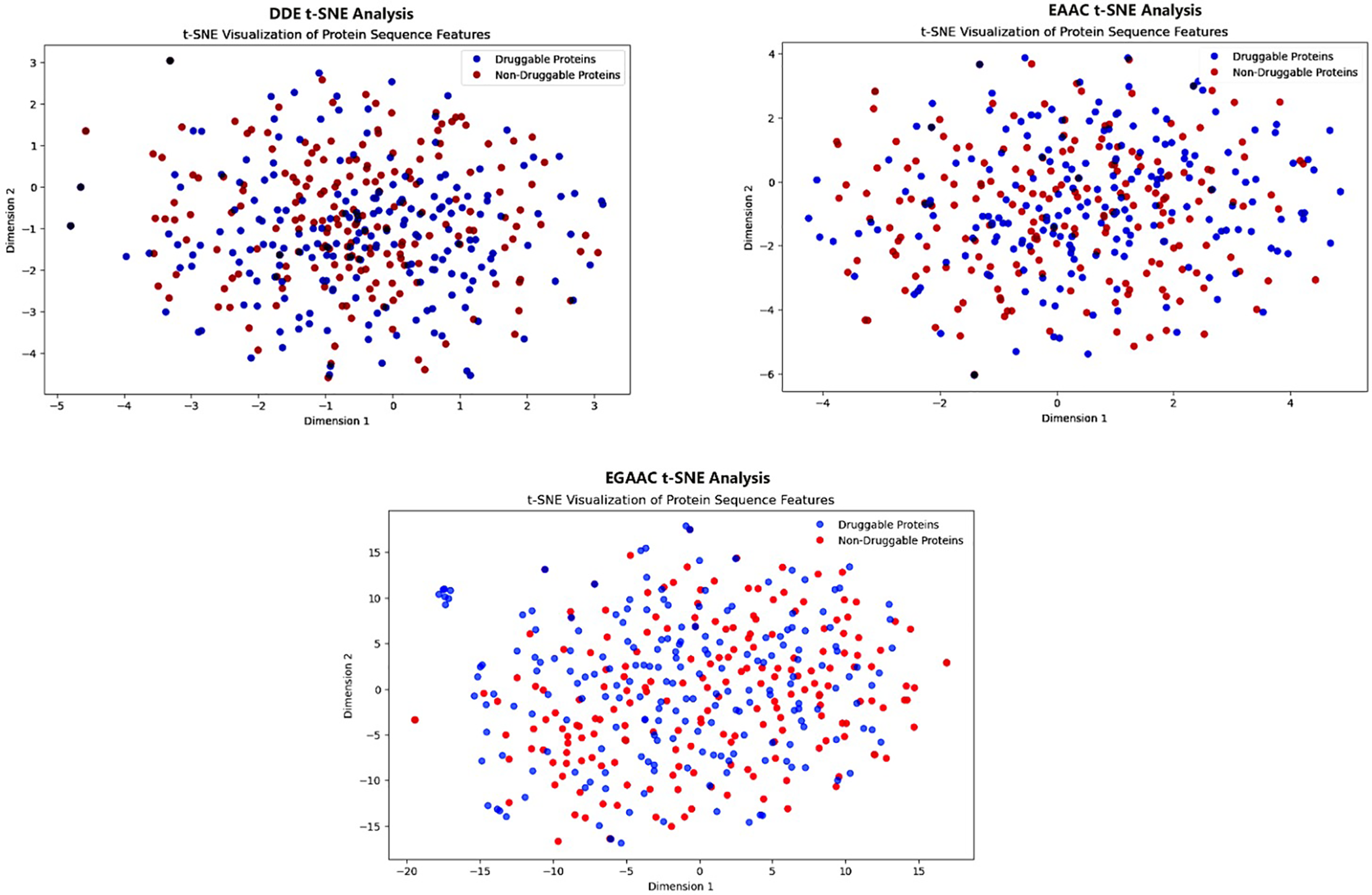
Figure 12: t-SNE Analysis (Bagging, Boosting, and Stacking)

4.9 PCA Feature Analysis for Druggable Protein Identification

To further analyze the underlying structure of the collected features and enhance the t-SNE and SHAP-based interpretations, Principal Component Analysis (PCA) was performed on all three feature types: DDE, EAAC, and EGAAC. PCA is a well-established linear dimensionality reduction method that converts high-dimensional data into a lower-dimensional space, preserving the directions of highest variance using orthogonal principle components [60].

Fig. 13 illustrates that the initial two principal components (PC1 and PC2) were employed to depict the class distribution across each feature set. Indicating that this descriptor captures discriminative patterns in the feature space, the PCA projection for DDE features showed a comparatively clearer separation between druggable and non-druggable proteins. Despite some reported class overlap in EAAC and EGAAC descriptors, significant grouping trends remained apparent. This indicates that even with a linear projection, the derived features retain class-relevant signals.

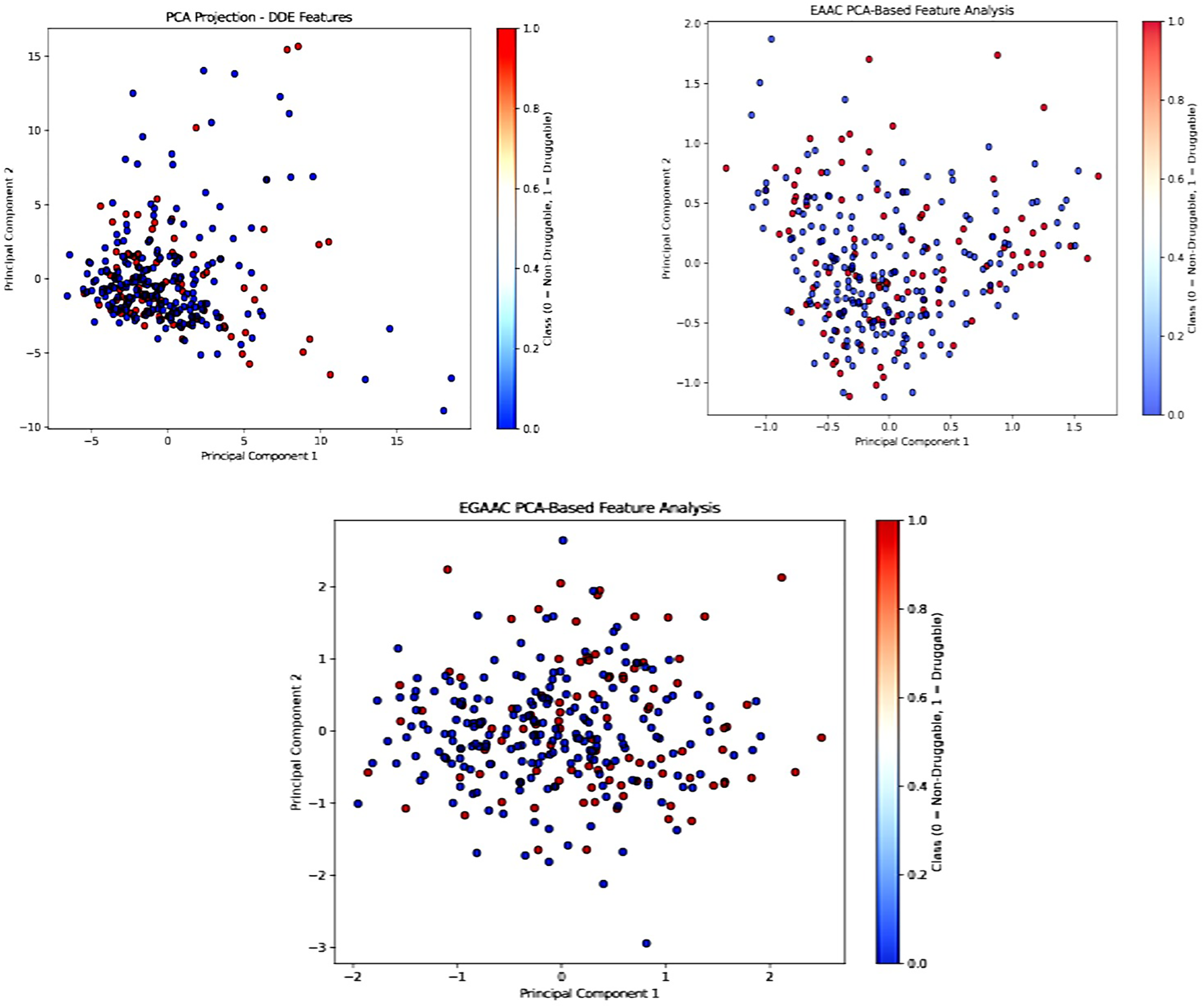
Figure 13: PCA analysis (Bagging, Boosting, and Stacking)

Although PCA may not properly represent intricate nonlinear manifolds like t-SNE, its linear projections provide an interpretable and complementary view of the spatial distribution of samples in the feature space. The congruence of PCA visualizations with t-SNE mappings and SHAP-derived feature importance substantiates the validity and consistency of our engineered feature sets across various interpretive dimensions, emphasizing the robustness of the proposed feature design strategy and its appropriateness for druggable protein prediction, even when assessed through different dimensionality reduction methodologies.

4.10 AUC-PR Curve Performance for Druggable Protein Identification

This figure shows how various models (Random Forest, Gradient Boosting, Support Vector Machine, Decision Tree, Logistic Regression, Voting (Soft), Stacking, Bagging) performed on the Precision-Recall (PR) curve. Each of these models has an AUC-PR score. Here is an overview of the AUC-PR comparison on all models. The best AUC-PR is achieved by RF, Voting (Soft), and Stacking (0.71 for all these models) in this competition. Bagging scores the worst with an AUC-PR of 0.61. Area Under the Precision-Recall Curve (AUC-PR) The AUC-PR is a performance metric used to evaluate how well a model can distinguish between positive and negative classes, particularly for imbalanced datasets, such as that employed in Druggable Protein Identification (refer to Fig. 14). The precision-recall curve (PR curve) allows us to understand to what degree the models are identifying the “druggable” proteins (positive class) vs. controlling the trade-off between minimizing the false positives (which are the proteins that are incorrectly labeled as druggable) and maximizing the precision (which is the correct recognition of druggable proteins). AUC-PR Curve Summary: Random Forest (AUC-PR = 0.71): It does a great job at retrieving the druggable proteins; the performance is high at all recall values. This indicates that RF does a good job of identifying druggable proteins while avoiding increasing the number of false positives. Gradient Boosting (AUC-PR = 0.69): The performance of this model is a bit lower than the Random Forest model, but it is still able to distinguish between druggable and non-druggable proteins quite well. Its performance isn’t as good as Random Forest at first glance, but it’s still good. SVM (AUC-PR = 0.63): Doesn’t crush Random Forest or Gradient Boosting, for sure. The plot visually demonstrates that it struggles in reducing the false positive rate, which translates into lower precision across different levels of recall. Decision Tree (A-UC-PR = 0.68): Better than SVM but not as good as Random Forest or Gradient Boosting. The curve indicates that the Decision Tree has difficulty in finding druggable proteins, especially when a large recall is achieved. Logistic Regression (AUC-PR = 0.65): It doesn’t work as well as the tree-based models (Random Forest, Gradient Boosting, Decision Tree). It has a smaller AUC-PR, indicating a less effective balance of precision and recall. Voting (Soft) (AUC-PR = 0.71): The Voting model (Soft) performs similarly to Random Forest. By applying a soft voting ensemble to average the predictions of multiple models, we can expect good performance while recognizing druggable proteins. Stacking (AUC-PR = 0.71): Stacking, similar to Voting (Soft), takes the best of a few models and has a good AUC-PR.

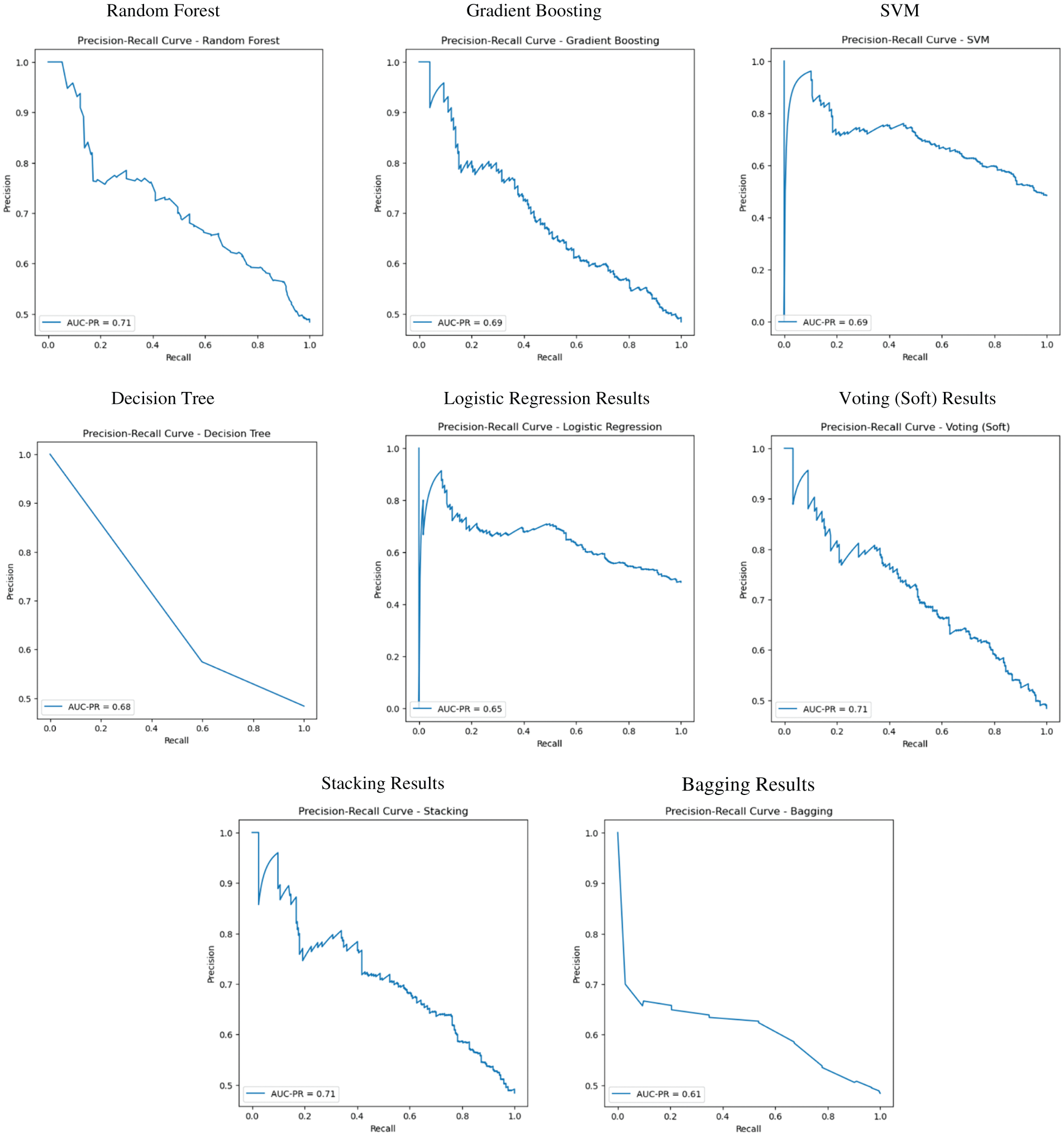
Figure 14: AUC-PR curve performance

Under this setting, the best performer in these figures, Random Forest and Voting (Soft), demonstrates similar results. Bagging (AUC-PR = 0.61): This model shows the lowest AUC-PR value, indicating lower AUC-PR value, which indicates less competitiveness and more false positives. This indicates that Drn can identify druggable proteins with more difficulty than the other models in the study. The models, such as Random Forest, Voting (Soft), and Stacking, perform the best in terms of predicting druggable proteins, with the AUC-PR score of 0.71. They strike the best balance between precision and recall, crucial for finding proteins that drugs can target. Bagging, in contrast, does horribly, with AUC-PR well lower, which implies it may not be as good at discovering druggable proteins.

4.11 AUC-PR Curve or MCC (Matthews Correlation Coefficient) Metrics for Druggable Protein Identification

Description of Table 7: Return on Capital, AUC-PR, and MCC (Matthews Correlation Coefficient) metric scores. This table displays the evaluation measures AUC-PR (Area Under the Precision-Recall Curve) and MCC (Matthews Correlation Coefficient) for various model performances. These metrics are frequently employed in machine learning to evaluate the efficacy of categorization algorithms. This is an analysis of the columns and values in the table:

The initial column, denoted by numbers 0 to 8, serves as an index that presumably signifies several models or experiments for which the metrics are calculated. This statistic assesses the balance between precision and recall at various thresholds, however the area under the curve (AUC) provides a comprehensive evaluation of model performance across all potential classification levels. Elevated AUC-PR values signify superior performance, with values approaching 1 denoting an ideal model and values nearing 0 reflecting subpar performance. MCC quantifies the quality of binary classifications. It considers both true positives and true negatives, and is seen as more relevant than other accuracy metrics when addressing imbalanced datasets. MCC values span from −1 to +1, with +1 denoting a flawless forecast, 0 signifying a random guess, and −1 representing a wholly erroneous prediction. MCC: 0.320107 A moderate MCC score, signifying acceptable model performance, if not exemplary. Analogous to the AUC-PR score, the MCC value is marginally lower, indicating a relatively diminished model performance. The MCC of 0.316226 surpasses that of Index 1, signifying a marginally superior classification accuracy. This table provides a summary of model performance across various metrics (AUC-PR and MCC). It emphasizes areas where specific models exhibit superior or inferior performance, and also illustrates the effect of absent data (NaN values) on various models.

5  Conclusions

The present investigation introduces a novel predictive framework for identifying druggable proteins. This framework leverages amino acid composition descriptors derived from protein sequences as input for three distinct Ensemble Learning Methods for Identification of Druggable Proteins (CEL-IDPs). The Stacking method is the most optimal method while utilizing a limited set of 400 dipeptide deviation from expected mean (DDE) amino acid composition characteristics.

The study identified the top 10 essential proteins in BC OncoOmics that are predicted to be druggable. These proteins include CDK4, AP1S1, POLE, HMMR, RPL5, PALB2, TIMP1, RPL22, NFKB1, and TOP2A. Additionally, the top 10 cancer-driving proteins that are predicted to be druggable were identified as TLL2, FAM47C, SAGE1, HTR1E, MACC1, ZFR2, VMA21, DUSP9, CTNNA3, and ABRG1. Lastly, the study also identified the top 10 RNA-binding proteins that are predicted to be druggable, which include PLA2G1B, CPEB2, NOL6, LRRC47, CTTN, CORO1A, SCAF11, KCTD12, and TMPO. However, the majority of these interventions currently need clinical trials. Ultimately, this robust model offers predictions for a number of proteins that have the potential to be targeted by drugs. These proteins warrant extensive investigation in order to identify more effective therapeutic targets and thereby enhance the efficacy of clinical trials.

This study presents a framework, CEL-IDP, which integrates sequence-derived features with three ensemble learning strategies. It identifies top druggable protein candidates and applies SHAP and t-SNE for model interpretability and visualization. Among all tested combinations, the ensemble models using EGAAC features, especially Bagging and Boosting, consistently achieved the highest accuracy, highlighting the robustness of these methods in predicting druggable proteins.

Various feature extraction algorithms can be employed to turn sequential nominal character information into a numerical vector. The enhancement of classification performance can be achieved through the extraction of efficient features. The following algorithms are utilized to extract characteristics from protein sequences: The EAAC refers to the increased amino acid composition. The improved grouped amino acid composition (EGAAC) and dipeptide deviation from expected mean (DDE) are two important factors to consider.

Clinical validation is required: Even though druggable proteins are predicted in this study, these targets still have to be tested through clinical trials for the proof of efficacy or relevance as therapeutic targets. Feature limitation: The model relies only on a limited set of 400 DDE amino acid composition attributes, which may be insufficient to capture the complexity of protein-drug association and is further limited by the magnitude of predictions. The generalizability of findings is limited by the focus of the study on specific sets of data, e.g., BC OncoOmics and cancer-driving proteins, limiting the usability of the model in other biological contexts or conditions. The approach depends heavily on sequence-based features, which might not fully capture other structural and dynamic features of proteins that may influence druggability.

Necessary for Further Examination: The top choice models and ensemble strategies (Bagging, Boosting, Stacking) all achieve superior accuracy, but the model needs more testing and refinement to ensure applicability to a broader range of proteins and conditions. Interpretability Shortcomings: SHAP and t-SNE enhance model interpretability, but still, they might not provide a complete or clear understanding of the complex relations natured in connection with these complex interactions between proteins and drugs or medicinal chemicals.

Acknowledgement: This research was supported by the MSIT (Ministry of Science and ICT), Korea, under the ITRC (Information Technology Research Centre) support program (IITP-2024-RS-2024-00437191) supervised by the IITP (Institute for Information & Communications Technology Planning & Evaluation).

Funding Statement: This research was supported by the MSIT (Ministry of Science and ICT), Korea, under the ITRC (Information Technology Research Centre) support program (IITP-2024-RS-2024-00437191) supervised by the IITP (Institute for Information & Communications Technology Planning & Evaluation).

Author Contributions: Conceptualization, Mujeebu Rehman and Qinghua Liu; methodology, Mujeebu Rehman and Ali Ghulam; software, Tariq Ahmad; validation, Mujeebu Rehman, Tariq Ahmad and Jawad Khan; formal analysis, Dildar Hussain; investigation, Jawad Khan; resources, Qinghua Liu; data curation, Yeong Hyeon Gu; writing original draft preparation, Mujeebu Rehman and Qinghua Liu; writing review and editing, Tariq Ahmad, Jawad Khan and Dildar Hussain; visualization, Mujeebu Rehman; supervision, Qinghua Liu; project administration, Qinghua Liu and Jawad Khan; funding acquisition, Dildar Hussain. All authors reviewed the results and approved the final version of the manuscript.

Availability of Data and Materials: We used the benchmark online freely available datasets that are mentioned in Section 2.

Ethics Approval: Not applicable.

Conflicts of Interest: The authors declare no conflicts of interest to report regarding the present study.

References

1. Kellner R. Proteomics. Concepts and perspectives. Fresenius’ J Anal Chem. 2000;366(6):517–24. doi:10.1007/s002160051547. [Google Scholar] [PubMed] [CrossRef]

2. Barbarino JM, Whirl-Carrillo M, Altman RB, Klein TE. PharmGKB: a worldwide resource for pharmacogenomic information. [cited 2025 Aug 12]. Available from: https://wires.onlinelibrary.wiley.com/doi/10.1002/wsbm.1417. [Google Scholar]

3. Whirl-Carrillo M, McDonagh EM, Hebert JM, Gong L, Sangkuhl K, Thorn CF, et al. Pharmacogenomics knowledge for personalized medicine. Clin Pharmacol Ther. 2012;92(4):414–7. doi:10.1038/clpt.2012.96. [Google Scholar] [PubMed] [CrossRef]

4. Vefghi A, Rahmati Z, Akbari M. Drug-target interaction/affinity prediction: deep learning models and advances review. Comput Biol Med. 2025;196(Pt A):110438. doi:10.1016/j.compbiomed.2025.110438. [Google Scholar] [PubMed] [CrossRef]

5. Ali N, Hanif N, Khan HA, Waseem MA, Saeed A, Zakir S, et al. Deep learning and artificial intelligence for drug discovery, application, challenge, and future perspectives. Discov Appl Sci. 2025;7(6):533. doi:10.1007/s42452-025-06991-6. [Google Scholar] [CrossRef]

6. Wang Y, Shi Z, Weerawarna P, Huang K, Richardson T, Wang Y. Building an explainable graph neural network by sparse learning for the drug-protein binding prediction. J Comput Biol. 2025;32(7):1–10. doi:10.1101/2023.08.28.555203. [Google Scholar] [CrossRef]

7. Charoenkwan P, Schaduangrat N, Moni MA, Shoombuatong W, Manavalan B. Computational prediction and interpretation of druggable proteins using a stacked ensemble-learning framework. iScience. 2022;25(9):104883. doi:10.1016/j.isci.2022.104883. [Google Scholar] [PubMed] [CrossRef]

8. Liu T, Altman RB. Identifying druggable targets by protein microenvironments matching: application to transcription factors. CPT Pharmacomet Syst Pharmacol. 2014;3(1):e93. doi:10.1038/psp.2013.66. [Google Scholar] [PubMed] [CrossRef]

9. Owens J. Determining druggability. Nat Rev Drug Discov. 2007;6(3):187. doi:10.1038/nrd2275. [Google Scholar] [CrossRef]

10. Sakharkar MK, Sakharkar KR, Pervaiz S. Druggability of human disease genes. Int J Biochem Cell Biol. 2007;39(6):1156–64. doi:10.1016/j.biocel.2007.02.018. [Google Scholar] [PubMed] [CrossRef]

11. Overington JP, Al-Lazikani B, Hopkins AL. How many drug targets are there? Nat Rev Drug Discov. 2006;5(12):993–6. doi:10.1038/nrd2199. [Google Scholar] [PubMed] [CrossRef]

12. Lindsay MA. Finding new drug targets in the 21st century. Drug Discov Today. 2005;10(23–24):1683–7. doi:10.1016/S1359-6446(05)03670-6. [Google Scholar] [PubMed] [CrossRef]

13. Cheng AC, Coleman RG, Smyth KT, Cao Q, Soulard P, Caffrey DR, et al. Structure-based maximal affinity model predicts small-molecule druggability. Nat Biotechnol. 2007;25(1):71–5. doi:10.1038/nbt1273. [Google Scholar] [PubMed] [CrossRef]

14. Gashaw I, Ellinghaus P, Sommer A, Asadullah K. What makes a good drug target? Drug Discov Today. 2011;16(23–24):1037–43. doi:10.1016/j.drudis.2011.09.007. [Google Scholar] [PubMed] [CrossRef]

15. Li Q, Lai L. Prediction of potential drug targets based on simple sequence properties. BMC Bioinform. 2007;8:353. doi:10.1186/1471-2105-8-353. [Google Scholar] [PubMed] [CrossRef]

16. Ding H, Takigawa I, Mamitsuka H, Zhu S. Similarity-based machine learning methods for predicting drug-target interactions: a brief review. Brief Bioinform. 2014;15(5):734–47. doi:10.1093/bib/bbt056. [Google Scholar] [PubMed] [CrossRef]

17. Huang C, Zhang R, Chen Z, Jiang Y, Shang Z, Sun P, et al. Predict potential drug targets from the ion channel proteins based on SVM. J Theor Biol. 2010;262(4):750–6. doi:10.1016/j.jtbi.2009.11.002. [Google Scholar] [PubMed] [CrossRef]

18. Carter AJ, Kraemer O, Zwick M, Mueller-Fahrnow A, Arrowsmith CH, Edwards AM. Target 2035: probing the human proteome. Drug Discov Today. 2019;24(11):2111–5. doi:10.1016/j.drudis.2019.06.020. [Google Scholar] [PubMed] [CrossRef]

19. Zhang M, Wan F, Liu T. DrugFinder: druggable protein identification model based on pre-trained models and evolutionary information. Algorithms. 2023;16(6):263. doi:10.3390/a16060263. [Google Scholar] [CrossRef]

20. Ackloo S, Antolin AA, Bartolome JM, Beck H, Bullock A, Betz UAK, et al. Target 2035—an update on private sector contributions. RSC Med Chem. 2023;14(6):1002–11. doi:10.1039/D2MD00441K. [Google Scholar] [PubMed] [CrossRef]

21. McCloskey K, Sigel EA, Kearnes S, Xue L, Tian X, Moccia D, et al. Machine learning on DNA-encoded libraries: a new paradigm for hit finding. J Med Chem. 2020;63(16):8857–66. doi:10.1021/acs.jmedchem.0c00452. [Google Scholar] [PubMed] [CrossRef]

22. Torng W, Biancofiore I, Oehler S, Xu J, Xu J, Watson I, et al. Deep learning approach for the discovery of tumor-targeting small organic ligands from DNA-encoded chemical libraries. ACS Omega. 2023;8(28):25090–100. doi:10.1021/acsomega.3c01775. [Google Scholar] [PubMed] [CrossRef]

23. Ahmad S, Xu J, Feng JA, Hutchinson A, Zeng H, Ghiabi P, et al. Discovery of a first-in-class small-molecule ligand for WDR91 using DNA-encoded chemical library selection followed by machine learning. J Med Chem. 2023;66(23):16051–61. doi:10.1021/acs.jmedchem.3c01471. [Google Scholar] [PubMed] [CrossRef]

24. Zhou Y, Chen SJ. Advances in machine-learning approaches to RNA-targeted drug design. Artif Intell Chem. 2024;2(1):100053. doi:10.1016/j.aichem.2024.100053. [Google Scholar] [PubMed] [CrossRef]

25. Volkamer A, Kuhn D, Grombacher T, Rippmann F, Rarey M. Combining global and local measures for structure-based druggability predictions. J Chem Inf Model. 2012;52(2):360–72. doi:10.1021/ci200454v. [Google Scholar] [PubMed] [CrossRef]

26. Dezső Z, Ceccarelli M. Machine learning prediction of oncology drug targets based on protein and network properties. BMC Bioinform. 2020;21(1):104. doi:10.1186/s12859-020-3442-9. [Google Scholar] [PubMed] [CrossRef]

27. Gong Y, Liao B, Wang P, Zou Q. DrugHybrid_BS: using hybrid feature combined with bagging-SVM to predict potentially druggable proteins. Front Pharmacol. 2021;12:771808. doi:10.3389/fphar.2021.771808. [Google Scholar] [PubMed] [CrossRef]

28. Sun T, Lai L, Pei J. Analysis of protein features and machine learning algorithms for prediction of druggable proteins. Quant Biol. 2018;6(4):334–43. doi:10.1007/s40484-018-0157-2. [Google Scholar] [CrossRef]

29. Yu L, Xue L, Liu F, Li Y, Jing R, Luo J. The applications of deep learning algorithms on in silico druggable proteins identification. J Adv Res. 2022;41:219–31. doi:10.1016/j.jare.2022.01.009. [Google Scholar] [PubMed] [CrossRef]

30. Butcher SP. Target discovery and validation in the post-genomic era. Neurochem Res. 2003;28(2):367–71. doi:10.1023/a:1022349805831. [Google Scholar] [PubMed] [CrossRef]

31. Müller S, Ackloo S, Al Chawaf A, Al-Lazikani B, Antolin A, Baell JB, et al. Target 2035—update on the quest for a probe for every protein. RSC Med Chem. 2022;13(1):13–21. doi:10.1039/d1md00228g. [Google Scholar] [PubMed] [CrossRef]

32. Jamali AA, Ferdousi R, Razzaghi S, Li J, Safdari R, Ebrahimie E. DrugMiner: comparative analysis of machine learning algorithms for prediction of potential druggable proteins. Drug Discov Today. 2016;21(5):718–24. doi:10.1016/j.drudis.2016.01.007. [Google Scholar] [PubMed] [CrossRef]

33. Bakheet TM, Doig AJ. Properties and identification of human protein drug targets. Bioinformatics. 2009;25(4):451–7. doi:10.1093/bioinformatics/btp002. [Google Scholar] [PubMed] [CrossRef]

34. Bhasin M, Raghava GPS. ESLpred: SVM-based method for subcellular localization of eukaryotic proteins using dipeptide composition and PSI-BLAST. Nucleic Acids Res. 2004;32:W414–9. doi:10.1093/nar/gkh350. [Google Scholar] [PubMed] [CrossRef]

35. Dhanda SK, Vir P, Raghava GPS. Designing of interferon-gamma inducing MHC class-II binders. Biol Direct. 2013;8:30. doi:10.1186/1745-6150-8-30. [Google Scholar] [PubMed] [CrossRef]

36. Saravanan V, Gautham N. Harnessing computational biology for exact linear B-cell epitope prediction: a novel amino acid composition-based feature descriptor. OMICS. 2015;19(10):648–58. doi:10.1089/omi.2015.0095. [Google Scholar] [PubMed] [CrossRef]

37. Chen Z, Zhao P, Li F, Leier A, Marquez-Lago TT, Wang Y, et al. iFeature: a Python package and web server for features extraction and selection from protein and peptide sequences. Bioinformatics. 2018;34(14):2499–502. doi:10.1093/bioinformatics/bty140. [Google Scholar] [PubMed] [CrossRef]

38. Lee TY, Lin ZQ, Hsieh SJ, Bretaña NA, Lu CT. Exploiting maximal dependence decomposition to identify conserved motifs from a group of aligned signal sequences. Bioinformatics. 2011;27(13):1780–7. doi:10.1093/bioinformatics/btr291. [Google Scholar] [PubMed] [CrossRef]

39. Yao L, Rzhetsky A. Quantitative systems-level determinants of human genes targeted by successful drugs. Genome Res. 2008;18(2):206–13. doi:10.1101/gr.6888208. [Google Scholar] [PubMed] [CrossRef]

40. Yıldırım MA, Goh KI, Cusick ME, Barabási AL, Vidal M. Drug-target network. Nat Biotechnol. 2007;25(10):1119–26. doi:10.1038/nbt1338. [Google Scholar] [PubMed] [CrossRef]

41. Cao DS, Xiao N, Xu QS, Chen AF. Rcpi: R/Bioconductor package to generate various descriptors of proteins, compounds and their interactions. Bioinformatics. 2015;31(2):279–81. doi:10.1093/bioinformatics/btu624. [Google Scholar] [PubMed] [CrossRef]

42. Hao J, Ho TK. Machine learning made easy: a review of Scikit-learn package in Python programming language. J Educ Behav Stat. 2019;44(3):348–61. doi:10.3102/1076998619832248. [Google Scholar] [CrossRef]

43. Breiman L. Bagging predictors. Mach Learn. 1996;24(2):123–40. doi:10.1007/BF00058655. [Google Scholar] [CrossRef]

44. Breiman L. Random forests. Mach Learn. 2001;45(1):5–32. doi:10.1023/A:1010933404324. [Google Scholar] [CrossRef]

45. Hughes G. On the mean accuracy of statistical pattern recognizers. IEEE Trans Inf Theory. 1968;14(1):55–63. doi:10.1109/TIT.1968.1054102. [Google Scholar] [CrossRef]

46. Friedman JH. Stochastic gradient boosting. Comput Stat Data Anal. 2002;38(4):367–78. doi:10.1016/S0167-9473(01)00065-2. [Google Scholar] [CrossRef]

47. Chen T, Guestrin C. XGBoost: a scalable tree boosting system. In: Proceedings of the 22nd ACM SIGKDD International Conference on Knowledge Discovery and Data Mining; 2016 Aug 13–17; San Francisco, CA, USA. p. 785–94. doi:10.1145/2939672.2939785. [Google Scholar] [CrossRef]

48. Brewka G. Artificial intelligence—a modern approach by Stuart Russell and Peter Norvig, Prentice Hall. Series in artificial intelligence, Englewood Cliffs, NJ. Knowl Eng Rev. 1996;11(1):78–9. doi:10.1017/s0269888900007724. [Google Scholar] [CrossRef]

49. Cover T, Hart P. Nearest neighbor pattern classification. IEEE Trans Inf Theory. 1967;13(1):21–7. doi:10.1109/TIT.1967.1053964. [Google Scholar] [CrossRef]

50. Swain PH, Hauska H. The decision tree classifier: design and potential. IEEE Trans Geosci Electron. 1977;15(3):142–7. doi:10.1109/TGE.1977.6498972. [Google Scholar] [CrossRef]

51. López-Cortés A, Paz-y-Miño C, Guerrero S, Cabrera-Andrade A, Barigye SJ, Munteanu CR, et al. OncoOmics approaches to reveal essential genes in breast cancer: a panoramic view from pathogenesis to precision medicine. Sci Rep. 2020;10:5285. doi:10.1038/s41598-020-62279-2. [Google Scholar] [PubMed] [CrossRef]

52. Repana D, Nulsen J, Dressler L, Bortolomeazzi M, Venkata SK, Tourna A, et al. The network of cancer genes (NCGa comprehensive catalogue of known and candidate cancer genes from cancer sequencing screens. Genome Biol. 2019;20(1):1. doi:10.1186/s13059-018-1612-0. [Google Scholar] [PubMed] [CrossRef]

53. Daanouni O, Cherradi B, Tmiri A. Predicting diabetes diseases using mixed data and supervised machine learning algorithms. In: Proceedings of the 4th International Conference on Smart City Applications; 2019 Oct 2–4; Casablanca, Morocco. p. 1–6. doi:10.1145/3368756.3369072. [Google Scholar] [CrossRef]

54. Nai-Arun N, Sittidech P. Ensemble learning model for diabetes classification. Adv Mater Res. 2014;931-932:1427–31. doi:10.4028/www.scientific.net/amr.931-932.1427. [Google Scholar] [CrossRef]

55. Mung PS, Phyu S. Ensemble learning method for enhancing healthcare classification. In: Proceedings of 2020 the 10th International Workshop on Computer Science and Engineering WCSE 2020; 2020 Jun 19–21; Shanghai, China. doi:10.18178/wcse.2020.02.024. [Google Scholar] [CrossRef]

56. Guerrero S, López-Cortés A, Indacochea A, García-Cárdenas JM, Zambrano AK, Cabrera-Andrade A, et al. Analysis of racial/ethnic representation in select basic and applied cancer research studies. Sci Rep. 2018;8:13978. doi:10.1038/s41598-018-32264-x. [Google Scholar] [PubMed] [CrossRef]

57. López-Cortés A, Paz-Y-Miño C, Guerrero S, Jaramillo-Koupermann G, León Cáceres Á, Intriago-Baldeón DP, et al. Pharmacogenomics, biomarker network, and allele frequencies in colorectal cancer. Pharmacogenom J. 2020;20(1):136–58. doi:10.1038/s41397-019-0102-4. [Google Scholar] [PubMed] [CrossRef]

58. Rodríguez-Pérez R, Bajorath J. Interpretation of machine learning models using shapley values: application to compound potency and multi-target activity predictions. J Comput Aided Mol Des. 2020;34(10):1013–26. doi:10.1007/s10822-020-00314-0. [Google Scholar] [PubMed] [CrossRef]

59. Xu X, Xie Z, Yang Z, Li D, Xu X. A t-SNE based classification approach to compositional microbiome data. Front Genet. 2020;11:620143. doi:10.3389/fgene.2020.620143. [Google Scholar] [PubMed] [CrossRef]

60. Mayer J, Jin Y, Wurster TH, Makowski MR, Kolbitsch C. Evaluation of synergistic image registration for motion-corrected coronary NaF-PET-MR. Philos Trans A Math Phys Eng Sci. 2021;379(2200):20200202. doi:10.1098/rsta.2020.0202. [Google Scholar] [PubMed] [CrossRef]