Requirements and Constraints of Forecasting Algorithms Required in Local Flexibility Markets

1  Introduction

The increasing use of renewable energy sources combined with increasing electricity demand has highlighted the importance of energy flexibility management in electrical grids [1]. Energy flexibility is the ability of the grid operator to manage variations in demand or generation, which is essential to ensure the stability and efficiency of the grid [2]. The Distribution System Operator (DSO) requires reliable electricity demand forecasts to, first, properly determine the occurrence of critical events (i.e., congestion or voltage variations) and, second, manage this flexibility (changes in generation or demand) to maintain the grid operating under safe conditions to guarantee the supply.

Smart grids represent a modern evolution in the management of electricity distribution and consumption, integrating advanced digital technologies into traditional power grids. They incorporate features such as smart meters, sensors, and automation systems to optimize grid operations, improve reliability, and accommodate the integration of renewable energy sources [3].

The European Council of Energy Regulators recommends that the DSO procurement of energy flexibility should be market-based [4], using local flexibility markets (LFMs) to trade flexibility locally between flexibility providers and DSOs. This market-based approach appears to be the most promising among the congestion management measures evaluated in [5]. Some studies provide compelling evidence that emerging flexibility market models represent a promising business with technical and economic justification [6].

Furthermore, in Europe, the digitalization of networks and smart metering implementations allows consumers and DSOs to know, close to real time, the consumption and generation patterns. This fact enables more accurate and efficient forecasting of consumption, at different time and spatial resolutions, which ultimately allows the DSOs to operate and manage the electrical grid more effectively.

This work analyses the challenges and requirements of forecast algorithms from the perspective of the different actors involved in flexibility trading through LFMs (commonly operated in a day-ahead basis), focusing on the role of DSOs. The DSO requires demand forecasts at different time scales and locations (i.e., voltage levels) in the grid, aiming to forecast critical events and launch flexibility-demand orders accordingly, as part of its mitigation strategy. Consumers and aggregators should respond to these flexibility demands with specific offers to reduce/increase the respective demand. So, they also require some forecasting capacity to elaborate proper flexibility offers; however, these have the additional advantage since they control (switch on/off, regulation, etc.) of the energy assets. Once the flexibility is traded (agreement between the different actors to increase/decrease demand at a specific time and point of the grid), there is still some time before its activation. In this scenario, short-time forecasting is commonly used to schedule flexible loads to optimally serve the agreed flexibility.

The accuracy of forecasts depends basically on the data quality (representativeness, resolution, availability, errors, etc.); however, market timings and current metering technologies impose constraints on data availability and consequently on the quality of models and these on the forecast results. The paper analyses the impact of market definition on the availability of data for both training the models and using them for forecasting.

2  Flexibility Markets: Background

2.1 Flexibility Concept, Actors and Products

Flexibility, in the electricity domain, is often defined as the ability to modify generation and/or consumption patterns, or demand, in response to an external signal to contribute to maintaining the stability of the power system cost-effectively [7]. This is exemplified by changing the amount and timing of energy use, as shown in Fig. 1, aiming to make the system more reliable, defer investments, reduce emissions, and/or reduce operational costs. Fig. 1 illustrates how the peak of demand in the morning and early afternoon can be reduced by activating flexibility, that is, incentivizing the consumer to move part of the demand to valley hours, resulting in a flatter curve and consequently in a more efficient system.

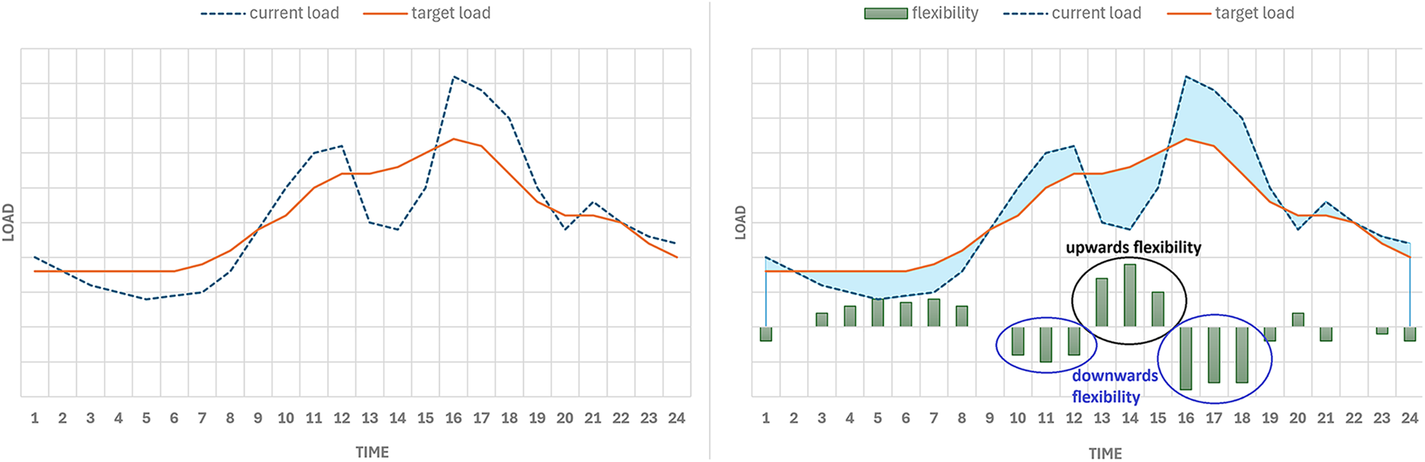
Figure 1: Concept of flexibility

Technically, flexibility is defined as a power change activated at a specified time for a specific duration at a particular node of the grid within the power distribution system. Thus, flexibility can be defined by five attributes [8]:

a)   Direction of flexibility (e.g., up or down).

b)   Rate of change (e.g., power capacity).

c)   Starting time and its trigger.

d)   Duration of the flexibility.

e)   Location (e.g, grid node, area, etc.)

Activation of flexibility can serve multiple purposes, and the goals together with the actors involved in the flexibility trading define the different markets and their operational rules. Thus, demandant of flexibility, i.e., the beneficiaries, are typically the Transmission System Operators (TSOs) and the DSOs, whereas the providers, those that have the capacity to balance generation and demand, are typically the producers and consumers.

The main actors involved in flexibility markets are [9]:

•   Transmission System Operator (TSO): responsible for the operation of the transmission system and its stability. TSO is a flexibility-demanding actor that requires flexibility to maintain energy balance and satisfy technical restrictions to guarantee system stability.

•   Distribution System Operator (DSO): responsible for the operation of the distribution system and power delivery to customers. It requires flexibility to avoid congestion, control voltage, and efficiently manage hosting capacity.

•   Balance Responsible Party (BRP): market entity (wholesale supplier or retailer) or its chosen representative, responsible for keeping its portfolio in balance. This is done by buying and selling energy with other market parties under the supervision of the grid and market operator.

•   Aggregator: acts as a facilitator between small entities providing flexibility (e.g., prosumers) and the market where minimal flexibility capacity is required. They offer aggregated flexibility that consumers can provide to the demanding partners.

•   Retailer: commercial entities that buy electric energy in the markets to be resold to their customers. Despite their role in energy trading, in some countries, they can also offer special products based on collaborative approaches similar to the aggregator.

Flexibility products are managed at different TSO-DSO levels supported by different flexibility markets [9]:

a)   Balancing at the transmission grid: Flexibility is offered to TSOs to correct imbalances between demand and supply in the electricity markets.

b)   Balancing at the distribution grid: Flexibility for the transmission grid, offered to TSOs for balancing purposes, but provided in the distribution grid by Distribution Energy Resource (DER) providers.

c)   Flexibility for the distribution grid: Flexibility products provided by DERs to DSOs for local balancing, voltage and congestion constraints, or reduction of losses. Proposals usually combine services to the DSOs as well as balancing services to the TSO, with hints on the coordination between both.

The first two categories, in the EU, are operated at different time frames through specific platforms according to availability requirements. These are typically known as Replacement Reserves (RR), Manual Frequency Restoration Reserves with Manual Activation (mFRR), and Restoration Reserves with Automatic Activation (aFRR), according to the harmonized market model definition. On the other hand, local market mechanisms for DSOs still have too low liquidity to be competitive, and their definition and operation depend on existing initiatives. However, the increasing electrification of heating and electromobility envisions the need for rapid development and expansion across the EU. This is the focus of this paper.

2.2 Local Flexibility Markets

A local flexibility market (LFM) can be defined as an electricity flexibility trading platform to trade flexibility in geographically limited areas such as neighborhoods, communities, towns and small cities [10]. There are some key aspects to consider to better understand the local flexibility markets [11]:

a)   Pre-qualification: It is the process imposed on flexibility assets and service providers to assess the level of complexity and any potential barriers to their participation in the local flexibility market. The process is divided into technical aspects (e.g., pre-qualification tests and other processes) and compliance with the necessary regulatory, legal, and/or financial requirements.

b)   Design of flexibility products: technical specifications of the flexibility products, such as the direction of the traded flexibility, horizon, and activation period, minimum bid size, notice period, time to full activation, and ramping limits.

c)   Trading of flexibility (market design): this considers how, and between which parties, flexibility products are traded.

d)   Activation and settlement procedures: these procedures encompass the communication means for the activation of flexibility services, verification of their execution, and billing.

The sequence of trading flexibility in an LFM, generally speaking, consists of three main stages [12]:

(1)   Contracting and bidding process: during this process, the DSO and flexibility providers (i.e., aggregator) reach an agreement for flexibility trading through an LFM operator. The result of the agreement includes quantity, time, location, and price of flexibility to be delivered. Flexibility demand is launched by the DSO some time (months, days, hours) before its expected activation. Flexibility demand is motivated by expected critical events in the grid, computed with forecast demand and generation together with grid models. Thus, the accuracy of forecast models is a crucial factor to estimate and elaborate flexibility demands (DSO side). Once the flexibility demand is launched to the market, elaboration of offers implies scheduling load/generation reserves by aggregators (or large prosumers/consumers).

(2)   Activation process: It consists of executing the procured flexibility by responding to a flexibility activation request with the increase or decrease of demand/generation according to agreed conditions. The aggregator (or prosumer) controls the energy assets (e.g., switch on/off of loads and/or DERs, charge/discharge of storage elements) to provide the amount of energy previously traded and under the agreed conditions (time, duration, quantity). The confirmation of the activation is communicated to the LFM operator by the aggregator, and the LFM operator confirms the flexibility provision to the DSO (and/or the BRP).

(3)   Settlement process: The flexibility transactions are completed through settlement arrangements and payment among the DSO, BRP, LFM operator, and aggregators/prosumers. The complexity resides in establishing the baseline from which the amount of activated flexibility is measured and verified. And, this baseline is defined based on forecasting models.

LFMs can operate at very different time frames (i.e., months in advance, day-ahead or intra-day) and they operate in parallel with the already existing energy and balancing markets [13]. Consequently, multiple forecast models, dealing with different time horizons and granularity, are required for flexibility trading.

2.2.1 Market Design and Definitions

The DSO is going to be the main buyer of flexibility in an LFM. Firstly, the DSO runs load flow analysis to investigate whether there is a future congestion or any other critical event. In order to run this load flow, accurate demand and generation forecasting is required. The more precision achieved in the forecasting, the more precise the load flow analysis will be, and, ultimately, the flexibility required will be able to solve more effectively the potential critical events in the grid. When the DSO forecasts a risk of critical events in the grid, it sends a request for flexibility to the LFM operator, including delivery information (location where flexibility is needed, type of problem, and system state). The LFM operator informs aggregators and market participants about the flexibility demanded, and these elaborate offers of flexibility accordingly. Finally, the LFM operator clears the market, and the results are sent to both the DSO and aggregators (Fig. 2).

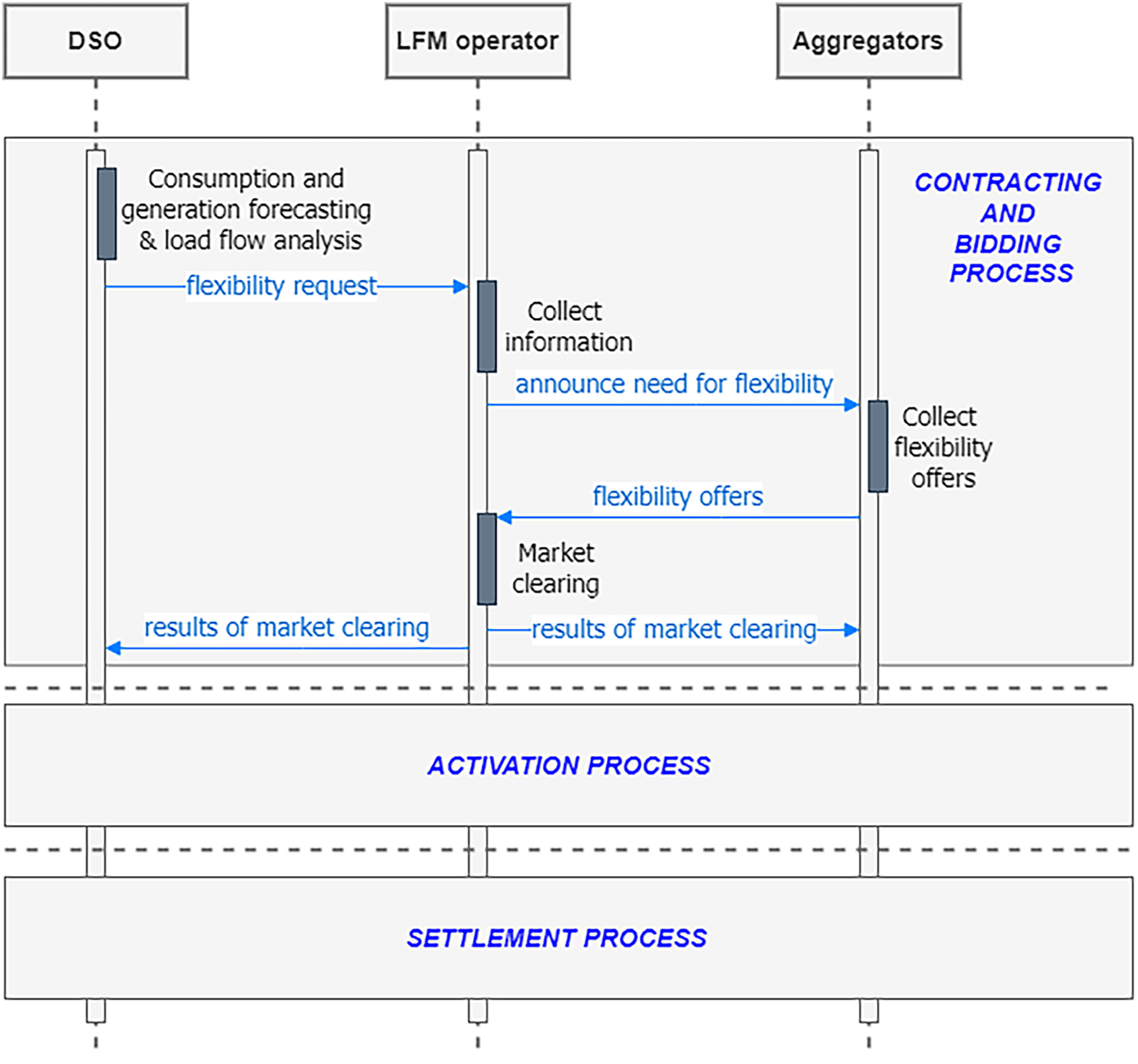
Figure 2: Sequence of trading flexibility in a local flexibility market

There are very few LFMs implemented and integrated into the existing EU electricity markets. However, there are promising initiatives covering interesting scenarios and products. One of the most representative is GOPACS, a TSO-DSO intermediary that allows for dealing with the coordination of grid operators outside of the market platform [14]. Basic characteristics include:

(1)   Pre-qualification: is the process of validating and accepting the flexibility provider. Participation in balancing markets usually implies the validation of the activation capacity and the availability of a real-time communication system, but in LFMs, this is usually less restrictive and does not include physical tests. In GOPACS, it takes a maximum of 5 working days.

(2)   Direction of flexibility offered goes both ways (upwards and downwards), and the minimum bid size is dictated by the intra-day market. Downwards flexibility means a consumption reduction, and it is commonly associated with positive values of flexibility (consumer view), whereas upwards is associated with an increase in generation (or alternatively a decrease in consumption) and it is assigned to negative values.

(3)   The market time unit (MTU): the minimum period of time for which the flexibility product price is established. It can vary, but common values are 15 min or 60 min, the same as in the wholesale intra-day market.

(4)   Starting of trading (tt): defines the time when the flexibility market opens and participants can start submitting their bids, or offers, for providing flexibility services. The market remains open until the closure time (tc).

(5)   Closure time (tc): Time instant when the flexibility market closes and does not accept new offers or changes.

(6)   Activation time (ta), deactivation time (td), and duration of activation (d=td−ta): times that define when flexibility is required to be activated after market clearance.

These concepts do not have a clear regulation and harmonization in the LFMs, and the multiple existing markets use different values (Fig. 3). There are LFMs where the start of trading begins 7 days before the time when flexibility services are required, others begin the trading 3 days before flexibility is required, while GOPACS begins a day before flexibility is needed. Gate closure time is also not unified, and every LFM sets distinct values for it; the same thing happens with the MTU (Fig. 3).

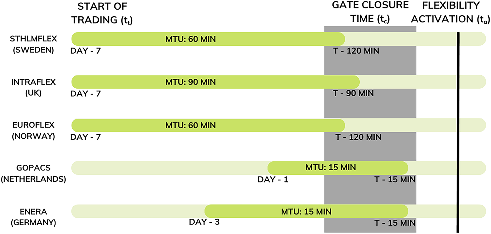
Figure 3: Local flexibility markets’ timings

Observe that the whole market is operated based on a forecasted demand, or baseline. Elaborating and agreement, among involved actors, on this baseline is a key factor in the flexibility trading process. The baseline represents how the net customer demand would be in the absence of the potential activation of flexibility according to some forecasting model. Estimation of the baseline, either by the DSO or the aggregator, is basically a forecasting problem constrained by the LFM market design and availability of data at every decision time. Thus, data granularity used in the forecasting models should be at least equal to MTU or shorter. Data availability before tt to forecast flexibility demand, at the DSO side (or before tc in case of aggregators or consumers/prosumers) influences the quality of the forecast at ta. And, the forecasting horizon is being defined by the difference ta−tt+d (or ta−tc+d for the consumer/prosumer).

2.2.2 Outline of Local Flexibility Markets in EU

There are a few LFMs currently operating in the EU. Some of the most representative are: Sthmlmflex (Sweden), IntraFlex (UK), NorFlex (Norway), GOPACS (Netherlands), Enera (Germany), UK tenders, and ENEDIS tenders (France). These initiatives were examined in [11], complementing in-depth desktop research with a survey and structured interviews with relevant stakeholders. Several key factors were considered to study the LFMs: pre-qualification procedures, the design of flexibility products, the trading of flexibility (procurement architecture), and the activation and settlement procedures.

A general conclusion in [15] states that there is not “one size fits all” design to manage congestion: characterizing and understanding the local context and needs before implementing new market or regulatory mechanisms is a prerequisite to ensure effectiveness and efficiency. LFMs address specific needs with different designs: it is, thus, unlikely that a unified/homogeneous design will emerge among European countries, although some common design principles and guidelines could emerge. Local market design from the DSO perspective is examined in [14], and they investigate the impact on technical infrastructure, network constraints, skill requirements, and regulatory rules. Based on them, an LFM framework is defined. In addition, Energy Networks Association has also designed a standard agreement for procuring flexibility services in [16].

Institutional implications of LFMs are discussed in [17]. They also analyze three discrimination concerns from the perspective of the network operator as a flexibility purchaser. Transparency policies on local flexibility markets are studied in [18]; and they claim that, in general, the forecast models for network congestion and LFM outcome are feasible. Nevertheless, the amount and quality of available information influence the performance of these forecasts. It can be expected that some market participants are better able to collect information than others. Therefore, an appropriate transparency policy should be designed as one major step when implementing LFMs, to provide a level playing field.

It was found in [19] that baseline services in LFMs do not meet the established requirements and that they are not compatible with the active participation of distributed energy resources in the power markets. Alternatively, they propose the use of limit-capacity services, which represent temporary absolute consumption caps for aggregators, and argue that they are better suited to tackle the challenges of distribution systems operation.

Key factors that impact the future of the local markets in Europe (with a focus on Sweden) are explored and ranked in [20]. The results show that the availability of active and smart end-users, and possible regulatory incentives for promoting the local markets, play important roles in the future of local markets. However, other impact factors in the future of local markets are the digitalization (availability of high-resolution data together with monitoring and control of medium & low voltage grids), the availability of distributed generation, and the controllability of loads (batteries, electrified mobility, and heating and cooling).

A fully functional local flexibility market under real conditions was designed and operated in the EcoGrid 2.0 project [21]. They assessed the benefits of baseline and capacity limitation services, showing that flexibility services in the distribution network can act as an insurance policy against network overload and outages. It was found in the study that aggregators can reliably deliver load reduction services on feeders with a large penetration of residential heating loads.

A local energy market (LEM) was simulated in [22], and it was found that the participation of a household without flexible assets would only be profitable for forecast errors below 30%–40%. They found in the literature review that the average forecast error for household loads is about 50%, which led them to consider participation in the LEM as not profitable, assuming state-of-the-art forecasting methods.

A paper demonstrates that predictions of significantly greater quality result in marginally higher value in terms of KPIs for the energy community in [23].

Authors in [24] propose a random forest-based method for building energy demand forecasting for 48 h ahead with a 15-min resolution adapted to the constraints imposed by LFMs. They utilize time-series decomposition to capture trend and seasonal components, combined with shape factor analysis to model grid load patterns.

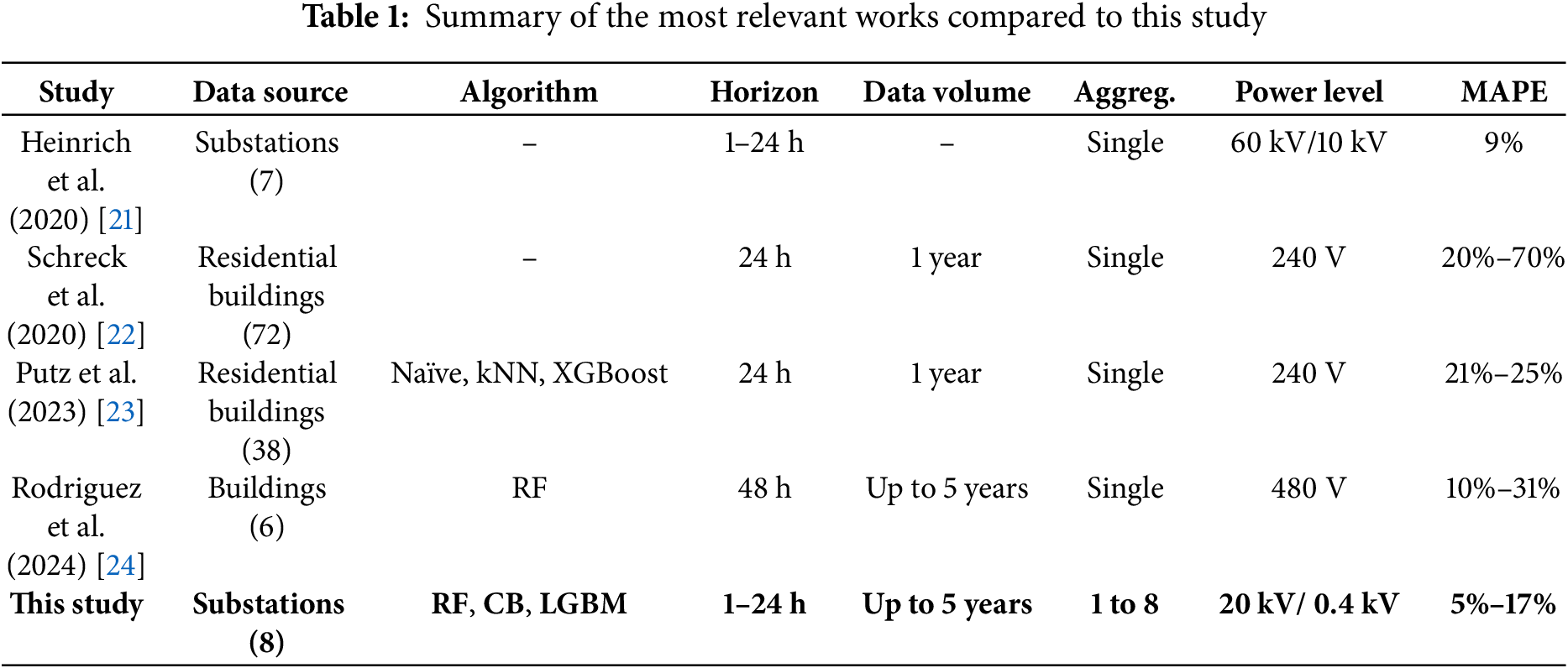
A comparison with the literature in Table 1 confirms the numerical validity of the proposed approach, which achieves similar results to the studies found. However, it is important to point out that due to the difference in datasets, the comparisons with the numerical results can only be indicative.

This study analyses the impact of local market definition on the requirements of forecasting algorithms. Forecasting is required by different actors and at different stages during market operation. DSOs, for instance, have access to smart metering infrastructure and can aggregate data according to grid topology, enabling more accurate forecasts of events such as congestion or over-voltages and the formulation of precise flexibility demands in LFMs. By contrast, aggregators typically rely on lower levels of aggregation, often under conditions of limited or less reliable data. Once the market closes and offers have been accepted, aggregators may further refine flexibility activation using short-horizon, household, or building-level forecasts. These differences highlight how data granularity and forecasting horizon critically shape the suitability of forecasting tools for flexibility provision in LFMs.

Despite the growing body of research on forecasting methodologies for energy systems, remarkably little attention has been paid to the requirements and constraints imposed by real-world data in LFM contexts. Most contributions emphasize novel model design or predictive accuracy under idealized datasets, while practical limitations such as granularity, heterogeneity, accessibility, aggregation level, and temporal resolution remain largely overlooked. To the best of our knowledge, studies explicitly examining how these data-related constraints influence the reliability of forecasting tools for LFMs are practically nonexistent. This gap is particularly problematic given that LFMs operate under stringent operational and temporal conditions, where forecasting is not an academic exercise but a prerequisite for market efficiency and stability. By addressing this issue, the present work contributes to the scientific discourse by aligning methodological advances with the operational realities of flexibility provision and activation in emerging LFMs.

3  The Challenge of Forecasting

Forecasting demand, generation, and flexibility (capability to change demand, or generation) is essential for the DSO to operate and manage electric power networks [9]. An energy forecast is also necessary to cope with risk management and to prevent potential congestion problems on the grid. To achieve this, several artificial intelligence (AI) methods are used.

However, there is no very well-defined structure for LFMs; studies found in the literature did things differently. Nevertheless, the forecasting timeframes in an LFM can be separated as such: short-term market and long-term market. Depending on the targeted market, the requirements of the forecasting algorithms differ. Algorithms for the short-term market require data close to real-time, while algorithms for the long-term market do not. Thus, data availability can be a huge factor in the short-term market for the algorithms to have a good performance.

There is another important factor to take into account, and that is data requirements. Studies found in the literature worked with different data requirements due to a lack of a well-defined guideline on how to operate an LFM. Forecasting algorithms can be heavily influenced depending on the availability of data, the frequency of each data sample, and the forecasting horizon. Thus, it is very important to establish clear and concise requirements of forecasting algorithms to participate in LFMs.

3.1 Formulation of the Forecasting Challenge

L(t) represents the net load demand at a specific point of the grid (e.g., feeder, transformer, or secondary substation). This can be considered as an aggregation of demand of individuals, li(t), in a specific area, Z, covered by the grid Eq. (1). Monitoring the evolution of L(t) is usually required to assess the loading of a transformer and support operation, maintenance, and investment planning.

L(t)=∑Zli(t)(1)

In that sense, forecasting this demand can help prevent critical events. Let us define L~t′(t) as the forecast of this demand at t, computed at t′. Usually, a forecast is not required for a single time instant but for a time interval, T, after t1 (t′<t1<t1+T), and the precision of this estimation is crucial to take the appropriate decisions. In general, the main factors affecting the accuracy of forecasts depend on the quality of the models, and this is influenced mainly by:

•   Representativeness of the data used when training the model. Thus, the calendar, weather, and historical energy data are usually the input of energy forecast models. However, more data does not always imply better results (forecasts of congestion events in summer probably are not correlated with winter demand).

•   Level of aggregation: As previously stated in Eq. (1), L(t) is the result of adding multiple individual and independent loads (and/or generations). If we assimilate these to continuous random variables, their addition results in a new variable that resembles a normal one, and the associated variance (in fact, time-varying variance) could be approximated by σ2L=∑σ2l⁢i (under the assumption that the individual variables are also normal). That means that the relative variability, in terms of σ, of aggregated demand is much lower than the addition of individual σ; and, consequently, the forecasting models improve with the level of aggregation.

•   Forecast horizon: The time separation between the time instants to forecast [t1,t1+T] and the instant when it is computed (t′) is very relevant. The correlation between samples of the random variable is highly influenced by their temporal distance. Thus, the demand at two consecutive hours is highly correlated. This also happens with the demand at the same time of the day in consecutive days; however, this is less true when trying to find relations between samples of different days at different hours or when considering different months (load demand in summer probably does not depend on the winter or spring demand).

Thus, forecasting to estimate critical events at the substation or transformer level requires using either data from a specific meter installed in the transformer or the aggregation of data from smart meters installed at the consumption points. Intuitively, it can be deduced that the longer the difference t1−t′ the greater the forecast error; and this interval basically depends on the market definition. According to previous LFMs definitions, t′ should correspond to tt and tc in the case of the DSO (flexibility demanding actor) and aggregator/prosumers (flexibility offering actor). However, this is not completely true since the availability of data either at tt or tc depends on how often metering devices report data. Therefore, two different data sources could be available to measure demand at the secondary substations: power measurements, available in near real time (seconds), through SCADAs; or hourly/quarterly energy data available daily through the Advanced Metering Infrastructure (AMI). Despite this, it is feasible to estimate energy demand from real-time power measurements. However, this is not commonly done because the level of instrumentation of secondary substations is still very limited (less than 10% of transformers at the secondary substations are instrumented). So, usually, energy metering data is used to estimate the demand, and this is affected by a low update ratio (typically once a day with hourly/quarterly granularity). This means that day-ahead forecasting can only benefit from data of the previous day (collected during today) (t1−t′>24h).

3.2 Forecasting Literature

Different methods and approaches have been found in the literature, and they can be classified into three main categories: statistical models [25,26], machine learning (ML) models [27–30], and deep learning (DL) models [31–34].

Statistical models aim to discover a mathematical relationship between the electricity consumption time series. We can mention models such as the Bayesian approach, the Autoregressive Moving Average, the Kalman filter, and the Gray methods. However, these algorithms are less accurate for long-term predictions, are highly susceptible to outliers in the dataset, and cannot handle the non-linear variation of energy data [35].

With the development of information technology, AI methods have replaced statistical models due to their abilities of learning features and processing data. Consequently, numerous studies and reviews on AI forecasting techniques have been conducted in the literature [36].

In [37], a comparison between conventional models and more recent AI models is made. Conventional models encompass time-series models (derived from auto-regressive and moving average models), regression models (linear, non-linear, logistic models), and gray models. For more recent ML and DL models, they consider Artificial Neural Network (ANN), Support Vector Regression (SVR), and Random Forest (RF). The conclusion drawn is that for daily and hourly energy consumption forecasting, more recent ML and DL-based models are more accurate than conventional models. Both ML and DL (a subcategory of ML) approaches require considerable amounts of data. In general, the more data available, the better the results will be [38]. Increasing input features of the model also improves the results if the features themselves are in some ways significant for the data model [38]. Therefore, data requirements play a big role in constructing an accurate model.

Three forecasting intervals, short, medium, and long-term, are reviewed in [39]. It is observed that most of the researches are conducted on short-term instead of medium and long-term. It is concluded in the research that a precise prediction will not only lead to notable decreases in penalties but also promote performance of various application fields, e.g., power grid maintenance and operating scheduling as well.

Reference [40] reviews the current state of the art of load forecasting models and draws several conclusions. Historical load data contributes to better model design, resulting in better accuracy and model performance. Every model has its own merits and demerits; however, hybrid methods were observed to have more performance efficiency in comparison to standalone methods. The hybridization of models with fine-tuned parameters had better performance. The short-term load forecasting is considered more reliable for operations and planning of utilities. It is also considered to further expand the operations and contribute in medium-term and long-term load forecasting.

In [41], the efficiency of hybrid models is discussed. The models put forward are: models based on Support Vector Machine (SVM) or Artificial Neural Networks (ANN) combined with Firefly Algorithm, Clustering Techniques, or Wavelet Transform, for instance.

An ML-prediction oriented review [42] exposes the superiority of eXtreme Gradient Boosting (XGB) methods compared to Multiple Linear Regression (MLR), ELastic Net (ELN), Random Forest (RF), Gradient Boosting Machines (GBM), or Support Vector Regression (SVR). In addition, the performance and accuracy of Deep Neural Network (DNN) models are praised in this research work.

DL has proven its ability to forecast time series. In particular, these models can be used to highlight inherent abstract characteristics and invariant structures in the data. Reference [43] provides a review of different DL methods such as Auto-encoder, DNN, Convolution Neural Network (CNN), and Recurrent Neural Network (RNN). The article highlights the interest of these models for feature extraction in demand forecasting, achieving good results with CNN for short-term forecasting.

Study [44] aims to optimize the performance of CNN, a model widely used in time-series forecasting. The conclusion drawn is that the smoothed CNN (a combination of exponential smoothing with CNN) outperforms other tested methods.

Other methods studied in the literature include Long Short-Term Memory (LSTM) methods. Reference [45] demonstrates the potential of using LSTM, attention-based LSTM, and Seq2Seq LSTM for multi-step prediction.

More recently, with the emergence of the attention mechanism and its integration into transformer models, the range of methods used to predict electricity consumption has been extended [46]. Initially used for natural language processing tasks, transformers are increasingly used for modeling time series. For instance, the Lag-Llama project [47], has been developed for non-limited prediction to a dataset. Lag-Llama is a foundational model built for univariate probabilistic time-series forecasting based on a decoder-only transformer architecture. It demonstrates strong results for 24-h prediction on unseen datasets and is able to achieve similar results compared to dataset-specific models.

Another hybrid model was developed in [48]. They propose a Self-Partitioning Local Neuro-Fuzzy (SPLNF) model based on Linear Neuro-Fuzzy models for short-term load forecasting, achieving better results than other tested methods, such as: seasonal auto-regressive integrated moving average (sARIMA), SVR, RF, and ANN.

3.3 Performance Evaluation Metrics

This work requires a comprehensive performance evaluation for Short-Term Load Forecasting (STLF). The appraisal involves the application of multiple evaluation metrics. MAE (Mean Absolute Error) is a measure of errors between paired observations expressing the same phenomenon (Eq. (2)).

MAE=∑t=1T|At−Ft|(2)

RMSE (Root Mean Square Error) is a commonly used metric for regression tasks since it penalizes large errors more heavily, making it sensitive to outliers (Eq. (3)).

RMSE=1T∑t=1T(At−Ft)2(3)

The sMAPE (symmetric Mean Absolute Percentage Error) (Eq. (4)) addresses some of the limitations of MAPE by applying a higher penalty to positive errors than to negative errors [49]. However, if the actual value is zero, the forecast is likely also close to zero. In such cases, the denominator in the formula approaches zero, which can lead to instability, so these instances are typically excluded from the calculation.

sMAPE=100T∑t=1T|Ft−At|(|At|+|Ft|)/2(4)

R2 (coefficient of determination) is a measure of how well the model explains the variance in the data; a high R2 value indicates a good fit of the model to the data (Eq. (5)).

R2=1−∑t=1T(At−Ft)2∑t=1T(At−y¯)2(5)

4  Case Study

In the short-term flexibility market, the forecasting requires data as close to real time as possible to forecast future consumption; timing specificities vary between LFMs as seen in Fig. 3. We study the impact on demand and generation forecasting of using different timings. Afterwards, we propose the most coherent and logical requirements for forecasting algorithms to participate in LFM according to market timings.

Literature review shows that DL methodologies are becoming really popular as of late due to their improved accuracy, robustness, and flexibility. State-of-the-art shows that deep neural networks, convolutional neural networks, and recurrent neural networks (specifically, the long short-term memory technique) are gaining a lot of traction.

In this study, RF, LightGBM (LGBM), and CatBoost (CB) [50] are evaluated to compare the effectiveness of the proposed forecasting model. The reasons for choosing these algorithms are that they have demonstrated to provide good performance to predict grid dynamics [51,52] and they provide a good trade-off between computational cost and accuracy. ANN-based algorithms were also tested (CNN, Auto-Encoders, LSTM), but were about ten times slower than RF, LGBM, and CB. Although the computational cost is not a severe constraint in this application domain, a faster response was prioritized in the selection of algorithms since it is important for decision makers (DSO operators).

RF is easy to interpret; each decision tree is a simple and transparent model, and they are relatively fast to train and predict. These facts make them suitable for large datasets. LGBM and CB are both popular machine learning algorithms, especially for gradient boosting, and they have gained widespread use in the data science and machine learning communities. These algorithms are remarkably optimized for speed and efficiency and incorporate various techniques to achieve high accuracy and robustness.

The case study takes place in Germany, data has been gathered in substations, and it was collected in the period of five years (from January 2018 to December 2022) with an hourly sampling rate. This data was collected during FEVER, an European Research & Innovation project. FEVER’s objective is to promote optimal management of the power grids in the future energy system based on renewable sources.

To carry out this study, we are going to consider the following scenarios:

1)   Time period for training: different periods of time are used to train the models to examine the best case scenarios (Section 5.1).

2)   Time horizon: the difference in accuracy between forecasting demand and generation before start of trading (next day forecasting) and after gate closure time (next hour forecasting) is studied (Section 5.2).

3)   Participant aggregation: it is studied how aggregating the points of data can impact the forecasting performance (Section 5.3).

4.1 Updated Process of Flexibility

The necessity for flexibility is forecasted by the DSO before the start of trading, which means that a longer horizon demand and generation forecasting is mandatory to estimate risks in the grid. Once gate closure time is reached and no more bids or offers can be submitted, the LFM operator clears the market and the results are sent to the DSO and aggregators (Fig. 2). However, we propose an additional step in the contracting and bidding process, right after the gate closure time and before the market clearing (Fig. 4). We suggest the DSO repeat the forecasting of demand and generation, repeat the load flow analysis, and update the flexibility required from aggregators. Forecasting the next day or forecasting the next hour can yield very different results. Thus, updating the forecast closer to real time could contribute substantially to improving forecasting performance. It is studied in detail whether the improvement of forecasting the next hour over the next day is enough to be considered as an additional step to implement in an LFM.

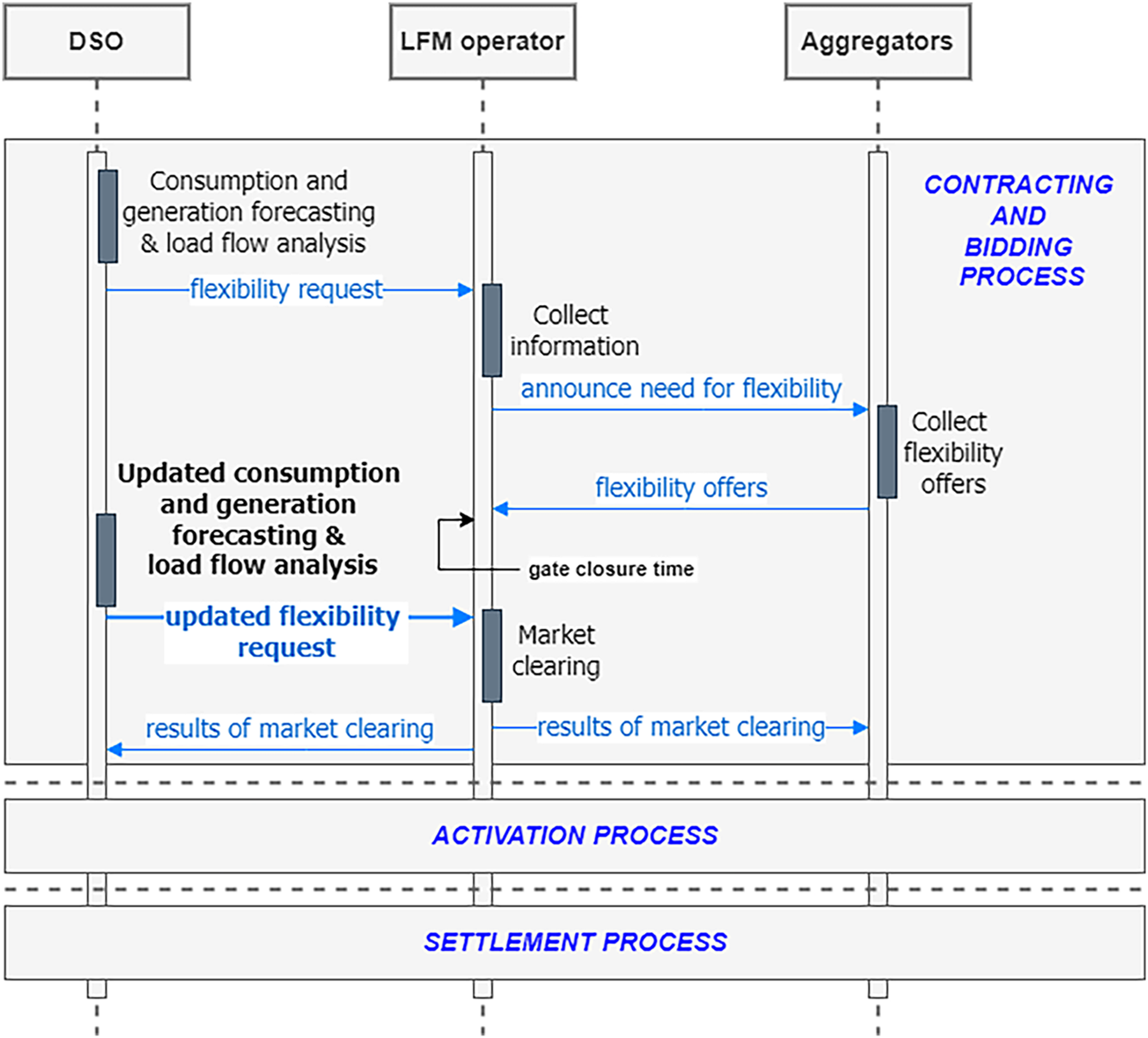
Figure 4: Proposal sequence of trading flexibility in a local flexibility market

4.2 Limitations

There is, however, a problem when it comes to forecasting the demand of individual participants of the LFMs. As per [22], the literature reveals that current forecast methodologies achieve an average forecast error of about 50% for individual household loads. This is an inherent limitation to individual household forecasting affected by human behavior.

Nevertheless, there are potential solutions to cope with this limitation. The implementation of a market mechanism with near-real-time trading of flexibility to give the possibility to compensate for forecast errors. Another solution is aggregating the participants of the LFM to reduce the combined forecast error. As mentioned, it is studied in detail how aggregating more participants of the LFM together can impact forecasting performance and help reduce the combined forecasting error. This way, however, the individual household is not the flexible asset anymore; the result of the aggregation becomes the flexible asset to manage.

4.3 Data

As mentioned, the data used for building the forecasting models is from the FEVER project (German pilot). We consider the data points from multiple substations as an aggregation of participants in an LFM and analyze how different operations on the dataset can positively affect the performance of the forecasting algorithms. Ultimately, improving forecasting performance is going to improve the quality of the flexibility procured, as seen in [23].

The data used in the study consisted of hourly electricity consumption data from multiple substations. Data does not contain missing values or any clear biases. Before modeling, the dataset undergoes a structured feature engineering process aimed at incorporating temporal dependencies and calendar effects into the predictive variables. Other features, such as forecasted temperature or forecasted solar radiation, have not been used as inputs because they would introduce an additional source of uncertainty in the results.

The primary predictive variables are constructed by generating lagged consumption values. For each timestamp, the consumption from the previous hours was extracted at varying lags ranging from one hour up to one week (e.g., 1 to 168 h prior—a week). Temporal calendar effects were incorporated by adding the day of the week and the month as categorical predictors. Additionally, a holiday indicator is generated, and it captures exogenous demand shifts due to non-working days.

A brief analysis of data used to train the models can be seen in Fig. 5. There are multiple clear, identifiable patterns, such as weekends having load demand profiles completely different than weekdays. Conversely, weekdays seem to have very similar load demand profiles. Weekends have considerably lower load demand than weekdays. This fact is accentuated on Sundays, which is the day of the week with the lowest load demand by a substantial margin, even when compared to Saturdays.

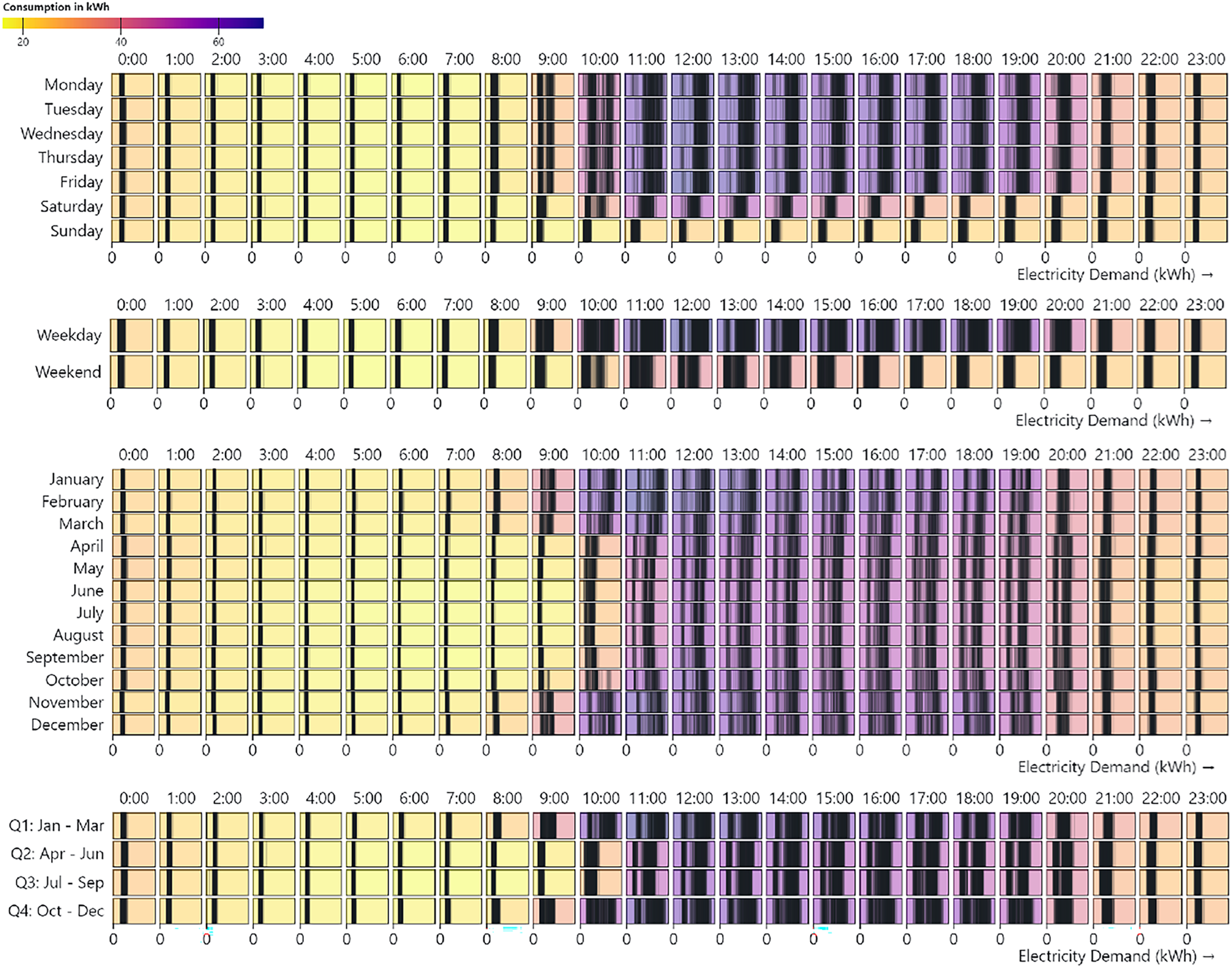
Figure 5: Distribution of load demand according to: different days of the week, weekdays or weekends, different months of the year and different quarters of the year

Similarly, load demand profiles seem to be higher early in the mornings during colder months, such as January, February, March, November, and December. This fact is also seen in the last plot of Fig. 5, where the hotter quarters have a lower load demand in the mornings. This phenomenon can be attributed to an increase in the use of heating, ventilation, and air conditioning (HVAC).

In [53], a period of time between 2000 and 2016 is studied, and it is concluded that colder winters can result in occasional consumption peaks. The warmest winters over the studied period concur with a decline in energy consumption. Conversely, 2010 represented one of the coldest years, and it coincides with a hike in energy consumption compared to other years.

Thus, the use of HVAC could be one of the factors causing this fluctuation of load demand profiles during the morning part of the day.

5  Results and Discussion

In this section, the results and performance metrics of the forecasting models, which are Random Forest, CatBoost and LightGBM, are presented. The evaluation results obtained for the models in the STLF are comprehensively discussed. Finally, based on their various performance metrics, a highlight of the best-performing prediction models is made.

The process of tuning the hyperparameters is carried out before the final performance evaluation of the models. Model training is performed within a randomized search framework using cross-validation. Specifically, for each candidate algorithm (RF, CB, and LGBM), a search space of key hyperparameters is defined (e.g., tree depth, learning rate, number of iterations, sub-sampling ratios, and regularization coefficients). Parameter combinations of these distributions are sampled and evaluated via 5-fold cross-validation. The hyperparameter configuration yielding the best validation performance is selected, and the final model to be evaluated is retrained on the full training set.

5.1 Data Volume Evaluation

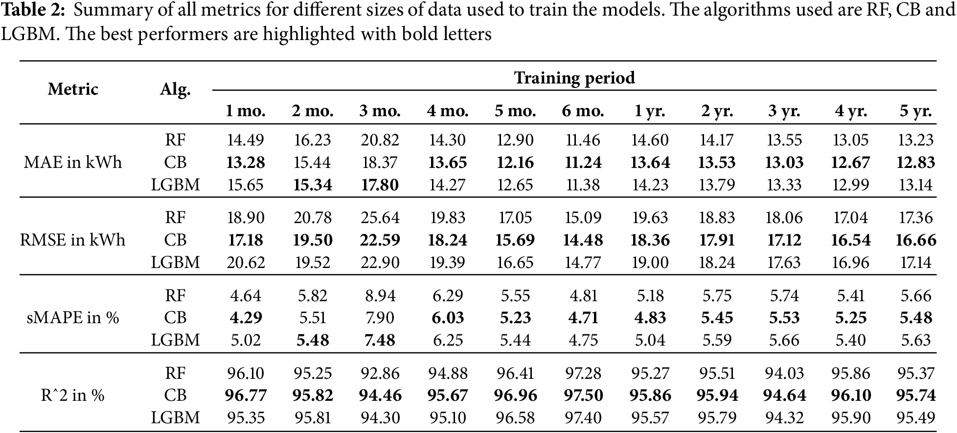
Having too much or too few data impacts the performance of the models for STLF. Surprisingly, the more data we have does not correlate with better metric values. Table 2 shows the evaluation metrics for each set of data. The shorter training periods seem to lead to worse results, with the exception of using 1 month to train, which achieves the best sMAPE value of 4.29%. This phenomenon seems to be contrary to what is expected in machine learning, although literature explicitly states that more data does not always mean better results [38].

The best R2 value is achieved by CB using 6 months of data, with a value of 97.50%. Furthermore, the same model also achieves the lowest MAE and RMSE values, 11.24 and 14.48 kWh, respectively. Notably, adding more data does not seem to improve results starting from the 6-month dataset onward.

In most cases, CB is obtaining the best results for the evaluated metrics, with exceptions on the 2 and 3-month training periods, where LightGBM has the advantage.

5.2 Time Horizon Evaluation

Evaluating the impact of different time horizons is crucial for an LFM. Due to the technical characteristics of the grid, an LFM can be limited to using certain time horizons, such as day-ahead or hour-ahead. STLF encompasses both hour-ahead and day-ahead forecasting. Results are shown in detail in Table 3.

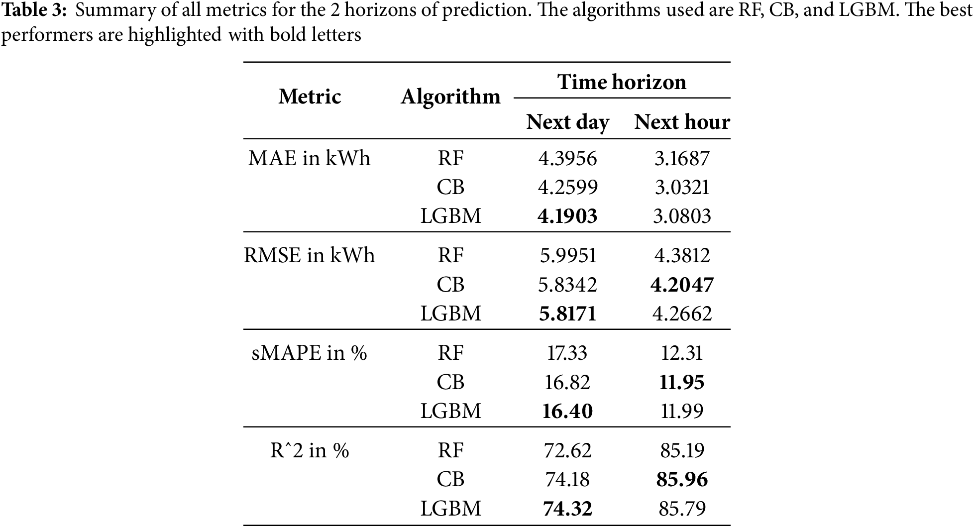
Unsurprisingly, the next hour time horizon achieves better results than the next day time horizon. The closer to real time approach has around 5% lower sMAPE than the day ahead approach, from 17% it goes to around 12% (depending on the forecasting method). The R2 metric also experiences a significant increase of around 12% in the hour ahead over the day ahead, from about 74% to 86%.

On another note, there is not a considerable difference between RF, CB, and LGBM algorithms. All three methods went through a process of hyperparameter tuning, and in the end, the variation between them seems to be negligible. However, LGBM takes advantage of next-day forecasting, and CB has the edge on next-hour forecasting.

5.3 LFM Participants Aggregation Evaluation

The results of aggregating participants are plotted in Fig. A3 and shown in Table 4. It shows a clear improvement in all metrics as more participants are aggregated together. The average sMAPE of each participant is about 12%, while the average sMAPE of all the participants aggregated together is about 6%. The R2 metric also shows a very steady increase as the participants are aggregated.

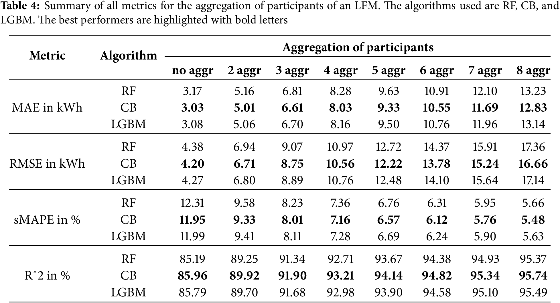
Nevertheless, MAE and RMSE values keep increasing as we aggregate more participants; this is due to the error being the average error. In reality, the MAE error for no aggregation should be the error committed by each participant multiplied by the number of participants (3kWh×8participants=24kWh). A MAE of 24 kWh when there is no aggregation is now in line with the MAE of 13 kWh when all participants are aggregated. Table 4 summarizes all error metrics regarding the aggregation of LFM participants.

5.4 Discussion

In this section, the previous results are examined in more detail, and multiple conclusions are reached from them. From the three cases we studied, there is a very clear winner when it comes to improving forecasting performance: aggregation of participants of the LFM.

Aggregating participants of an LFM seems to be really worthwhile since it increases the forecasting accuracy dramatically. Aggregating the participants together improves our sMAPE metric by about 100%, and R2 metric improves by 16% approximately. This is a sizable increase in forecasting performance just from the fact of aggregating participants together and treating them as a single unit. However, smaller aggregations such as 2-participant aggregation or 3-participant aggregation also seem to be worth considering.

Based on these results, the existence of data close to real time has a hefty impact on the accuracy of the forecasts, about 40% improvement in forecasting accuracy. This increase in forecasting accuracy could be significant enough to consider updating the flexibility request once gate closure time has been reached. This additional step, which consists of updating the flexibility request, is precisely what is proposed in Section 4.1 (Fig. 4).

On another note, training the models with half a year of data manages to obtain the best results. However, this could change in other scenarios and participants’ data. Training with half a year captures best the load consumption behaviors, but using smaller datasets, such as 1 month or 2 months, could also be considered. The accuracy of models trained with more data, such as 1 year to 5 years, does not beat the models with half a year of data, although we have seen in the literature that adding more data generally tends to positively impact the quality of the models. This could be due to the fact that load patterns change substantially over the course of the years, household appliances could have become more efficient with time, new necessities that require electricity consumption arise, households installing more and more DERs, etc.

6  Conclusions

This study delves into the requirements and constraints of forecasting algorithms in order to participate in the emerging local flexibility markets. Specifically, different data characteristics are analyzed throughout this paper to find out the performance impact it has on the STLF models. STLF models used in this work are Random Forest, CatBoost, and LightGBM. Through a methodical fine-tuning of the model parameters, we intend to increase the models’ accuracy and provide more precise and trustworthy load forecasts. Taken together, the analysis suggests the following trends and insights.

Firstly, adding more data to train the models does not always imply higher forecasting accuracy. While it is generally true that the bigger the dataset, the higher the model performance, in this case, it does not seem to follow this trend. This fact can be attributed to data having seasonal characteristics, even monthly characteristics. A forecasting model trained with summer data is going to be completely different than a forecasting model trained with winter data; consumption patterns are going to be entirely distinct. CatBoost seems to be the most accurate one in most of the training periods, with certain exceptions where LightGBM takes the lead.

Secondly, forecasting the next hour’s consumption is indeed more accurate than forecasting the entire next day’s consumption. The closer in time we are to the value we want to predict, the easier it is for the forecasting models. In the next hour horizon, CatBoost takes the lead, whereas LightGBM takes the edge on the next day horizon.

Thirdly, the more participants of the LFM that are aggregated together, the higher the performance of the STLF models. The accuracy of the models is improved by about 100%, going from no aggregation to aggregating 8 participants together. Additionally, CatBoost also takes the lead in this case study, in all sets of aggregation of participants.

Overall, these results provide compelling evidence that data requirements can play a pivotal role in LFMs. Forecasting algorithms need to be meticulously trained in order to be as accurate as possible, resulting in better flexibility procurement in the LFM. Finally, this paper has found that LFM in Spain is still in an infancy stage, with regulatory barriers hindering its development. As the regulatory landscape evolves, it is likely that LFMs will play a crucial role in Spain’s transition to a low-carbon economy. Thus, taking into consideration the results obtained in this paper could help propose a better framework to develop efficient and robust LFMs in Spain.

Future research avenues may delve further into the integration of additional time resolutions to the dataset to analyze how it impacts the accuracy and robustness of STLF models. Forecasting the hour-ahead demand with smaller resolutions, such as 15-min, could influence the accuracy of the models. The local flexibility markets seem to be moving towards this 15-min resolution. Current local flexibility markets that use this resolution are GOPACS and Enera.

Acknowledgement: The authors would like to thank the FEVER project—Flexible Energy Production, Demand and Storage-Based Virtual Power Plants for Electricity Markets and Resilient DSO Operation—for contributing to the data used in this work.

Funding Statement: This research was funded by RESCHOOL, grant agreement No. 101096490. The work had continuity within the RESCHOOL project—Strategies and Tools for Incentivization and Management of Flexibility in Energy Communities with Distributed Resources—aiming to analyze the capacity of energy communities to participate in local flexibility markets.

Author Contributions: Alex Segura: Data Acquisition and Analysis, Investigation, Methodology, Formal Analysis, Software, Validation, Visualization, Writing–Original Draft. Joaquim Meléndez: Conceptualization and Design of This Study, Supervision, Study Review, Writing–Review and Editing. All authors reviewed the results and approved the final version of the manuscript.

Availability of Data and Materials: Due to the nature of this research, participants of this study did not agree for their data to be shared publicly, so supporting data is not available.

Ethics Approval: Not applicable.

Conflicts of Interest: The authors declare no conflicts of interest to report regarding the present study.

Appendix A

See Figs. A1–A3.

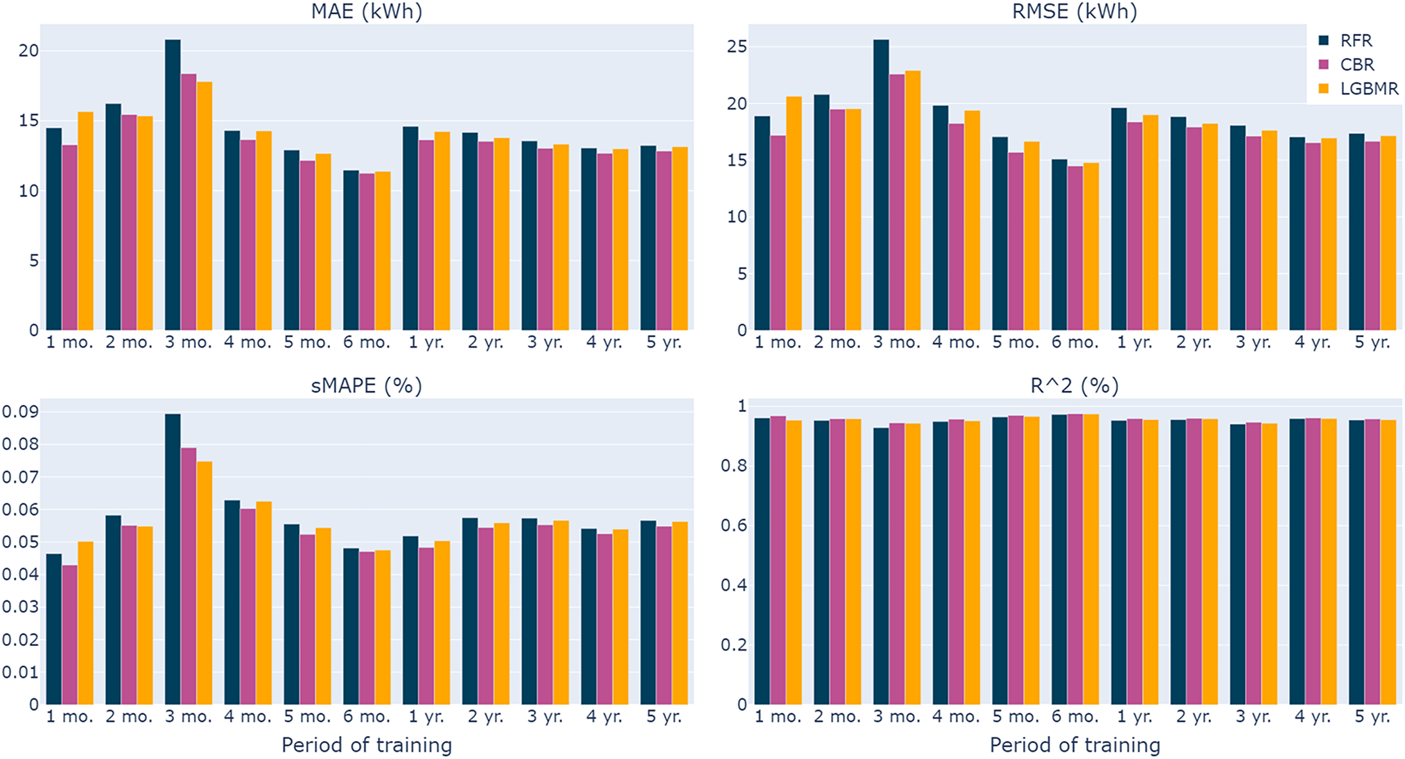
Figure A1: Training data volume comparison. The algorithms used are RF, CB, and LGBM. Different datasets are generated to train the models for each period of time, starting model training with 1 month of data and increasing the amount of data until the model training uses 5 years of data

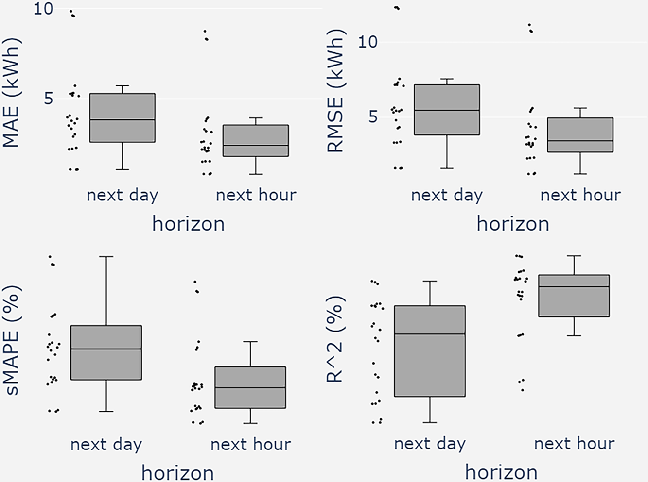
Figure A2: LFM closure time comparison: hour ahead vs. day ahead. The algorithms used are RF, CB, and LGBM. Each box-point represents a trained model (RF, CB, or LGBM) for a participant

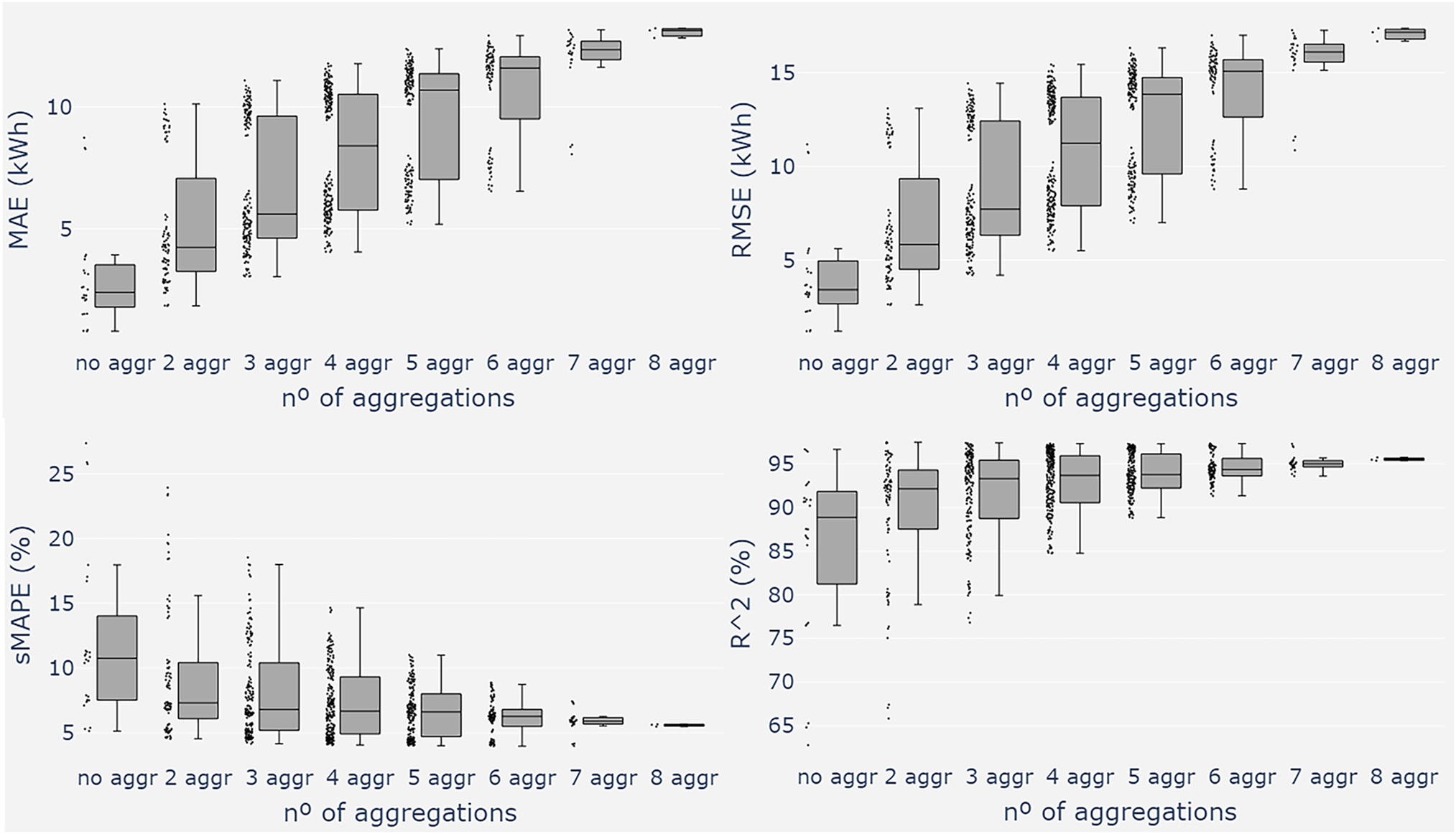
Figure A3: Demand aggregation comparison. The algorithms used are RF, CB, and LGBM. Each box-point represents a trained model (RF, CB, or LGBM) with a possible aggregation combination of the participants

References

1. Guchhait R, Sarkar B. Increasing growth of renewable energy: a state of art. Energies. 2023;16(6):2665. doi:10.3390/en16062665. [Google Scholar] [CrossRef]

2. Hussain S, Lai C, Eicker U. Flexibility: literature review on concepts, modeling, and provision method in smart grid. Sustain Energy Grids Netw. 2023;35(1):101113. doi:10.1016/j.segan.2023.101113. [Google Scholar] [CrossRef]

3. Bayindir R, Hossain E, Vadi S. The path of the smart grid -the new and improved power grid. In: 2016 International Smart Grid Workshop and Certificate Program (ISGWCP). Istanbul, Turkey: IEEE; 2016. p. 1–8. [Google Scholar]

4. Regulatory recommendations for the deployment of flexibility. In: EG3 report. Washington, DC, USA: Smart Grid Task Force; 2015. EU SGTF-EG3. 2015. [Google Scholar]

5. Kulms T, Meinerzhagen AK, Koopmann S, Schnettler A. Development of an agent-based model for assessing the market and grid oriented operation of distributed energy resources. Energy Proc. 2017;135:294–303. doi:10.1016/j.egypro.2017.09.521. [Google Scholar] [CrossRef]

6. Valarezo O, Gómez T, Chaves-Avila JP, Lind L, Correa M, Ulrich Ziegler D, et al. Analysis of new flexibility market models in Europe. Energies. 2021;14(12):3521. doi:10.3390/en14123521. [Google Scholar] [CrossRef]

7. Ma J, Silva V, Belhomme R, Kirschen DS, Ochoa LF. Evaluating and planning flexibility in sustainable power systems. IEEE Trans Sustain Energy. 2013;4(1):200–9. doi:10.1109/tste.2012.2212471. [Google Scholar] [CrossRef]

8. Eid C, Codani P, Perez Y, Reneses J, Hakvoort R. Managing electric flexibility from distributed energy resources: a review of incentives for market design. Renew Sustain Energy Rev. 2016;64:237–47. doi:10.1016/j.rser.2016.06.008. [Google Scholar] [CrossRef]

9. Villar J, Bessa R, Matos M. Flexibility products and markets: literature review. Electric Power Syst Res. 2018;154:329–40. doi:10.1016/j.epsr.2017.09.005. [Google Scholar] [CrossRef]

10. Olivella-Rosell P, Bullich-Massagué E, Aragüés-Peñalba M, Sumper A, Ødegaard Ottesen S, Vidal-Clos JA, et al. Optimization problem for meeting distribution system operator requests in local flexibility markets with distributed energy resources. Appl Energy. 2018;210(4):881–95. doi:10.1016/j.apenergy.2017.08.136. [Google Scholar] [CrossRef]

11. Stamatios C, Julija V, Antonios M, Ioulia P, Gianluca F. Local electricity flexibility markets in Europe. Luxembourg: Publications Office of the European Union; 2022. KJ-NA-31-194-EN-N. [Google Scholar]

12. Jin X, Wu Q, Jia H. Local flexibility markets: literature review on concepts, models and clearing methods. Appl Energy. 2020;261(1):114387. doi:10.1016/j.apenergy.2019.114387. [Google Scholar] [CrossRef]

13. Torbaghan SS, Blaauwbroek N, Nguyen P, Gibescu M. Local market framework for exploiting flexibility from the end users. In: 13th International Conference on the European Energy Market (EEM); 2016 Jun 6–9; Porto, Portugal. p. 1–6. [Google Scholar]

14. Honarmand ME, Hosseinnezhad V, Hayes B, Siano P. Local energy trading in future distribution systems. Energies. 2021;14(11):3110. doi:10.3390/en14113110. [Google Scholar] [CrossRef]

15. Dronne T, Roques F, Saguan M. Local flexibility markets for distribution network congestion-management in Center-Western Europe: which design for which needs? Energies. 2021;14(14):4113. doi:10.3390/en14144113. [Google Scholar] [CrossRef]

16. Association EN. Flexibility services standard agreement; 2023 [Internet]. [cited 2024 Mar 22]. Available from: https://www.energynetworks.org/publications/ena-on-standard-agreement-for-procuring-flexibility-services-07-sep-2023. [Google Scholar]

17. Buchmann M. How decentralization drives a change of the institutional framework on the distribution grid level in the electricity sector–the case of local congestion markets. Energy Policy. 2020;145(2013):111725. doi:10.1016/j.enpol.2020.111725. [Google Scholar] [CrossRef]

18. Heilmann E. The impact of transparency policies on local flexibility markets in electric distribution networks. Util Policy. 2023;83:101592. doi:10.1016/j.jup.2023.101592. [Google Scholar] [CrossRef]

19. Ziras C, Heinrich C, Bindner HW. Why baselines are not suited for local flexibility markets. Renew Sustain Energ Rev. 2021;135(1):110357. doi:10.1016/j.rser.2020.110357. [Google Scholar] [CrossRef]

20. Alavijeh NM, Ghazvini MAF, Steen D, Tuan LA, Carlson O. Key drivers and future scenarios of local energy and flexibility markets. In: 2021 IEEE Madrid PowerTech; 2021 Jun 28–Jul 2; Madrid, Spain. p. 1–6. [Google Scholar]

21. Heinrich C, Ziras C, Syrri ALA, Bindner HW. EcoGrid 2.0: a large-scale field trial of a local flexibility market. Appl Energy. 2020;261(4):114399. doi:10.1016/j.apenergy.2019.114399. [Google Scholar] [CrossRef]

22. Schreck S, Prieur de La Comble I, Thiem S, Niessen S. A methodological framework to support load forecast error assessment in local energy markets. IEEE Trans Smart Grid. 2020;11(4):3212–20. doi:10.1109/tsg.2020.2971339. [Google Scholar] [CrossRef]

23. Putz D, Gumhalter M, Auer H. The true value of a forecast: assessing the impact of accuracy on local energy communities. Sustain Energy Grids Netw. 2023;33(2):100983. doi:10.1016/j.segan.2022.100983. [Google Scholar] [CrossRef]

24. Rodriguez F, Maqueda E, Fernandez M, Pimenta P, Marques MI. A novel methodology for day-ahead buildings energy demand forecasting to provide flexibility services in energy markets. Int J Electr Power Energy Syst. 2024;161(6):110207. doi:10.1016/j.ijepes.2024.110207. [Google Scholar] [CrossRef]

25. Güngör O, Akşanlı B, Aydoğan R. Algorithm selection and combining multiple learners for residential energy prediction. Future Gen Comput Syst. 2019;99(3):391–400. doi:10.1016/j.future.2019.04.018. [Google Scholar] [CrossRef]

26. Massana J, Pous C, Burgas L, Melendez J, Colomer J. Short-term load forecasting in a non-residential building contrasting models and attributes. Energy Buildings. 2015;92(5):322–30. doi:10.1016/j.enbuild.2015.02.007. [Google Scholar] [CrossRef]

27. Huang Y, Yuan Y, Chen H, Wang J, Guo Y, Ahmad T. A novel energy demand prediction strategy for residential buildings based on ensemble learning. Energy Procedia. 2019;158:3411–6. doi:10.1016/j.egypro.2019.01.935. [Google Scholar] [CrossRef]

28. Divina F, García Torres M, Goméz Vela FA, Vázquez Noguera JL. A comparative study of time series forecasting methods for short term electric energy consumption prediction in smart buildings. Energies. 2019;12(10):1934. doi:10.3390/en12101934. [Google Scholar] [CrossRef]

29. Jiang B, Cheng Z, Hao Q, Ma N. A building energy consumption prediction method based on random forest and ARMA. In: 2018 Chinese Automation Congress (CAC); 2018 Nov 30–Dec 2, Xi’an, China. p. 3550–5. [Google Scholar]

30. Wang Z, Wang Y, Zeng R, Srinivasan RS, Ahrentzen S. Random forest based hourly building energy prediction. Energy Buildings. 2018;171(2):11–25. doi:10.1016/j.enbuild.2018.04.008. [Google Scholar] [CrossRef]

31. Sülo I, Keskin SR, Dogan G, Brown T. Energy efficient smart buildings: LSTM neural networks for time series prediction. In: 2019 International Conference on Deep Learning and Machine Learning in Emerging Applications (Deep-ML); 2019 Aug 26–28; Istanbul, Turkey. p. 18–22. [Google Scholar]

32. Marino DL, Amarasinghe K, Manic M. Building energy load forecasting using deep neural networks. In: IECON 2016-42nd Annual Conference of the IEEE Industrial Electronics Society; 2016 Oct 23–26; Florence, Italy. p. 7046–51. [Google Scholar]

33. Mlangeni S, Ezugwu AE, Chiroma H. Deep learning model for forecasting institutional building energy consumption. In: Conference on Information Communications Technology and Society (ICTAS); 2020 Mar 11–12; Durban, South Africa. p. 1–8. [Google Scholar]

34. Mocanu E, Nguyen PH, Gibescu M, Kling WL. Deep learning for estimating building energy consumption. Sustain Energy Grids Netw. 2016;6(4):91–9. doi:10.1016/j.segan.2016.02.005. [Google Scholar] [CrossRef]

35. Khalil M, McGough AS, Pourmirza Z, Pazhoohesh M, Walker S. Deep learning and statistical analysis for forecasting building energy consumption—a systematic review. Eng Appl Artif Intell. 2022;115(11):105287. doi:10.1016/j.engappai.2022.105287. [Google Scholar] [CrossRef]

36. Barja-Martinez S, Aragüés-Peñalba M, Munné-Collado Í, Lloret-Gallego P, Bullich-Massagué E, Villafafila-Robles R. Artificial intelligence techniques for enabling Big Data services in distribution networks: a review. Renew Sustain Energ Rev. 2021;150:111459. doi:10.1016/j.rser.2021.111459. [Google Scholar] [CrossRef]

37. Wei N, Li C, Peng X, Zeng F, Lu X. Conventional models and artificial intelligence-based models for energy consumption forecasting: a review. J Pet Sci Eng. 2019;181(11):106187. doi:10.1016/j.petrol.2019.106187. [Google Scholar] [CrossRef]

38. Kariluoto A, Kultanen J, Soininen J, Pärnänen A, Abrahamsson P. Quality of data in machine learning. In: 2021 IEEE 21st International Conference on Software Quality, Reliability and Security Companion (QRS-C); 2021 Dec 6–10; Hainan, China. p. 216–21. [Google Scholar]

39. Ahmad T, Zhang H, Yan B. A review on renewable energy and electricity requirement forecasting models for smart grid and buildings. Sustain Cities Soc. 2020;55(1):102052. doi:10.1016/j.scs.2020.102052. [Google Scholar] [CrossRef]

40. Azeem A, Ismail I, Jameel SM, Harindran VR. Electrical load forecasting models for different generation modalities: a review. IEEE Access. 2021;9:142239–63. doi:10.1109/access.2021.3120731. [Google Scholar] [CrossRef]

41. Mamun A, Sohel M, Sami NM, Sunny MS, Roy D, Hossain E. A comprehensive review of the load forecasting techniques using single and hybrid predictive models. IEEE Access. 2020;8:134911–39. doi:10.1109/access.2020.3010702. [Google Scholar] [CrossRef]

42. Fan C, Xiao L, Zhao Y. A short-term building cooling load prediction method using deep learning algorithms. Appl Energy. 2017;195(3):222–33. doi:10.1016/j.apenergy.2017.03.064. [Google Scholar] [CrossRef]

43. Wang H, Lei Z, Zhang X, Zhou B, Peng J. A review of deep learning for renewable energy forecasting. Energy Convers Manag. 2019;198(11):111799. doi:10.1016/j.enconman.2019.111799. [Google Scholar] [CrossRef]

44. Wibawa A, Putra Utama AB, Elmunsyah H, Pujianto U, Dwiyanto F, Hernandez L. Time-series analysis with smoothed convolutional neural network. J Big Data. 2022;9(1):44. doi:10.1186/s40537-022-00599-y. [Google Scholar] [PubMed] [CrossRef]

45. Lindemann B, Müller T, Vietz H, Jazdi N, Weyrich M. A survey on long short-term memory networks for time series prediction. Procedia CIRP. 2021;99(2):650–5. doi:10.1016/j.procir.2021.03.088. [Google Scholar] [CrossRef]

46. Vaswani A, Shazeer N, Parmar N, Uszkoreit J, Jones L, Gomez AN, et al. Attention is all you need. arXiv:1706.03762. 2023. [Google Scholar]

47. Rasul K, Ashok A, Williams AR, Ghonia H, Bhagwatkar R, Khorasani A, et al. Lag-Llama: towards foundation models for probabilistic time series forecasting. arXiv:2310.08278. 2024. [Google Scholar]

48. Tavassoli-Hojati Z, Ghaderi SF, Iranmanesh H, Hilber P, Shayesteh E. A self-partitioning local neuro fuzzy model for short-term load forecasting in smart grids. Energy. 2020;199(4):117514. doi:10.1016/j.energy.2020.117514. [Google Scholar] [CrossRef]

49. Makridakis S, Hibon M. The M3-Competition: results, conclusions and implications. Int J Forecast. 2000;16(4):451–76. doi:10.1016/s0169-2070(00)00057-1. [Google Scholar] [CrossRef]

50. Zhang L, Jánošík D. Enhanced short-term load forecasting with hybrid machine learning models: CatBoost and XGBoost approaches. Expert Syst Appl. 2024;241(4):122686. doi:10.1016/j.eswa.2023.122686. [Google Scholar] [CrossRef]

51. Mallala B, Khan PA, Pattepu B, Eega PR. Integrated energy management and load forecasting using machine learning. In: 2024 2nd International Conference on Sustainable Computing and Smart Systems (ICSCSS); 2024 Jul 10–12; Coimbatore, India. p. 1004–9. [Google Scholar]

52. Mallala B, Ahmed AIU, Pamidi SV, Faruque MO, Reddy R. Forecasting global sustainable energy from renewable sources using random forest algorithm. Results Eng. 2025;25(17):103789. doi:10.1016/j.rineng.2024.103789. [Google Scholar] [CrossRef]

53. Tsemekidi Tzeiranaki S, Bertoldi P, Diluiso F, Castellazzi L, Economidou M, Labanca N, et al. Analysis of the EU residential energy consumption: trends and determinants. Energies. 2019;12(6):1065. doi:10.3390/en12061065. [Google Scholar] [CrossRef]