Rheological Properties of Solid Rocket Propellants Based on Machine Learning

1  Introduction

The propellant for domestic sports rockets is generally a high-solid content suspension with solid fillers such as Ap and aluminum powder as the dispersed phase and liquids such as binders and plasticizers as the continuous phase. The flowability of the slurry is an important indicator for characterizing the quality of the propellant column in diesel engines and is also a major influencing factor that must be considered in the design of related mechanical equipment. In particular, the rheological properties of the propellant slurry play a decisive role in the production of solid rocket motors, since they directly affect key processes such as casting, molding, degassing, and curing. Poor rheological control can lead to defects such as voids, cracks, or uneven density distribution, which in turn compromise the structural integrity and performance reliability of the motor. As a high-solid-content thermosetting composite material, propellant slurry exhibits high viscosity at low shear rates and a significant reduction in viscosity at high shear rates. Its rheological behavior conforms to the characteristics of shear thinning in non-Newtonian fluids. Therefore, when studying the rheological properties of propellant slurry, it is often regarded as a non-Newtonian fluid for research.

In recent years, many scholars have been conducting experimental research on the rheological properties of propellants. Du et al. [1] conducted viscosity, yield stress, and thixotropic ring tests on two typical hydroxyl butyrate propellant slurries, obtaining rheological performance-time curves and infrared spectra at different curing times for the two slurries, and investigated the dynamic and static mechanical properties of the cured drug column. Yue et al. [2] conducted Computational Fluid Dynamics (CFD) simulation and numerical simulation studies on the pressure rod falling ball viscometer and verified the feasibility of the simulation results through experiments. Through the simulation results, it was found that the shear stress of the falling ball in the solution was very small, and the shear rate of the solution during the falling ball process was very low. It was concluded that the falling ball method could accurately determine the static viscosity of the slurry. Hoque et al. [3] used a shear rheometer and a power-law model (k, n) to fit and compare P01/P02: Both showed shear thinning (n < 1), and P01 had a higher consistency index and yield stress. The curing kinetics shows that toluene diisocyanate (TDI) is faster than isophorone diisocyanate (IPDI), and the Arrhenius activation energy is consistent with this. The theoretical pouring rate of vacuum casting at different temperatures was evaluated by using the non-Newtonian modified Hargen-Poiseuille equation. Yue et al. [4] studied the steady-state rheological properties of hydroxyl terminated polybutadiene (HTPB) solid propellant using a rotational rheometer and conducted numerical simulations. The results indicated that the solid propellant slurry had yield pseudoplasticity. Wang et al. [5] conducted leveling experiments on the propellant slurry after it was placed for different periods of time using a leveling instrument, and studied the porosity of the domestic propellant through CT scanning. The results showed that as the placement time of the slurry increased, the leveling property of the slurry decreased and the porosity increased. Wang and Qiang [6] conducted tensile tests on HTPB-based composite propellants under different confining pressures. By analyzing the mechanical properties of the propellants under different confining pressures and combining with the double shear strength theory, a new strength criterion was proposed to analyze the failure criterion of propellant aging. Yuan et al. [7] compared the rheological properties of hydroxyl-terminated polyether (HTPE) and HTPE/Polycaprolactone (PCL) four-component propellant slurps at different temperatures and shear rates using a rheometer. It was analyzed that the shear stress and shear rate of the propellant slurps showed an exponential growth within a certain range, and the slurps were pseudoplastic. Zhou et al. [8] studied the casting process by using the Carreau model to simulate it, explored the law of pore disappearance, and verified it through experiments.

Most existing studies focus on single-factor or steady-state rheological characterization, while paying insufficient attention to the multi-factor coupling nonlinear relationship between the viscosity of propellants and their dependent variables (shear rate, temperature, premix time). Especially during the pouring process, process Settings such as temperature and premixed time can significantly alter the microstructure and macroscopic viscosity of the slurry, thereby affecting the mold filling flow and the formation of forming defects. The system reveals and models this nonlinear mapping, which not only enhances the credibility and predictability of the numerical simulation of the pouring process, but also provides a quantitative basis for the optimization of process parameters, thereby reducing porosity, improving the forming quality of the drug column and enhancing batch-based consistency.

There exists a rather complex nonlinear relationship between the viscosity of the propellant slurry fluid and its influencing factors. BP neural networks have a strong fitting ability [9], but due to backpropagation, neural networks are easily affected by factors such as initial values, thresholds, and weights, resulting in insufficient generalization ability of the algorithm, low solution accuracy, poor learning rate, and getting stuck in local optima. In recent years, in order to prevent BP neural networks from falling into local optimum, many scholars have utilized intelligent algorithms to optimize the structure of the network, thereby enhancing the global optimization ability of the algorithm. In high-cost engineering design, adaptive Kriging-assisted RBMDO reduces PE/FEA calls while maintaining reliability [10]. In demanding HCI settings, a bat-algorithm–enhanced BPNN mitigates local minima and improves robustness [11]. In railway dynamics, an ANN surrogate efficiently predicts weld-induced wheel–rail impact forces, showcasing the advantage of data-driven modeling [12]. For wind-turbine support structures, a portfolio-based hybrid RBDO with Kriging accelerates surrogate construction and iterations, shortening the optimization cycle [13]. At the meta-heuristic level, RGAOA rebalances exploration–exploitation via Runge–Kutta and golden-sine strategies, improving convergence and stability [14]. At the optimizer level, Lion is more compute-efficient than Adam and offers practical guidance for BPNN training and learning-rate choices [15]. Moreover, Tian et al. [16] provides complementary evidence from another intelligent-optimization/model-refinement route, indicating that architecture/hyperparameter search or tailored training strategies can further strengthen BPNN’s global optimization and practical deployment [16]. Although the introduced optimization algorithms such as particle swarm optimization algorithm [17,18], genetic algorithm, grey Wolf optimization [19], whale algorithm [20], Particle Swarm Optimization [21] and other algorithms [22–24] can improve the accuracy of the network, they may also experience low algorithm accuracy and fall into local optimum in complex environments such as nonlinearity. Inspired by a series of natural behaviors of sparrows such as intelligent foraging and anti-predation, Xue and Shen [25] proposed the sparrow search algorithm SSA, which outperforms other algorithms such as the gray Wolf algorithm, particle swarm optimization algorithm, and gravitational search algorithm in dealing with complex nonlinear problems.

The viscosity of solid rocket propellants is affected by factors such as shear rate, temperature and time, and its expression is a complex nonlinear problem. In this paper, BP is optimized by combining the SSA and GA algorithms, and a prediction model for the kinematic viscosity of propellant slurry fluid based on the SSA-GA-BP method is proposed for the viscosity prediction of propellant slurry. The response surface method was adopted to fit and obtain a suitable surrogate model, expressing the explicit relationship among shear rate, temperature and time. Response surface methodology (RSM) has been successfully applied to engineering optimization, including geothermal system optimization [26] and bioenergy production [27]. Building on this, recent surrogate-modeling advances—such as hybrid adaptive Kriging integrated with water-cycle algorithms [28]—and comprehensive surveys on evolutionary computation for expensive optimization [29] underscore the promise of surrogate-based approaches for nonlinear, high-fidelity simulations. Specific techniques, including multi-fidelity Kriging and Kriging-assisted evolutionary optimization [30], further enhance efficiency and accuracy, and these methods have been extended to multidisciplinary design and structural integrity analysis [31]. Based on this, the response surface method was adopted to fit and obtain a suitable surrogate model, expressing the explicit relationship among shear rate, temperature and time. This provides a method for the viscosity prediction of propellant slurry fluids with the same proportioning components and also for the application of the optimized neural network method in the viscosity prediction of the same series of propellant slurries. The flowchart of the research approach in this paper is shown in Fig. 1.

Figure 1: Flowchart of research ideas

2  Theoretical Model

2.1 Constitutive Model of Non-Newtonian Fluids

Given that solid rocket propellants contain a high proportion of solid fillers and form complex dispersion systems, they usually exhibit non-Newtonian fluid characteristics. Especially when the continuous phase itself is a viscoelastic non-Newtonian fluid, the rheological properties of the entire dispersion system become even more complex. When describing the viscosity characteristics of viscoelastic fluids, common models include the power-law model, the Carreau model, and the Cross model. Their expressions are respectively shown in Eqs. (1)–(3):

Power-law model:

η=Kγ˙n−1(1)

In the formula, γ˙ is the shear rate; K is the viscosity coefficient; n is the index of flow behavior.

Carreau model:

η(γ˙)=η∞+(η0−η∞)(1+(λγ˙)2)n−12(2)

In the formula, η0 is the zero shear viscosity of the fluid; η∞ is the infinite shear viscosity of the fluid; λ is a time constant.

Cross model:

η(γ˙)=η01+(λγ˙)m1+(λγ˙)n(3)

The power-law model, the Cross model and the Carreau model are all constitutive models of viscoelastic fluids based on empirical formulas. In engineering, they are often the preferred viscosity models for shear-thinning fluids such as propellant slurries.

2.2 The Basic Principle of BP Neural Network

BP (Back Propagation) neural network is a concept proposed by scientists led by Rumelhart [32] in 1986. Its idea is to imitate the working principle of the human brain and construct a mathematical model. It is a multi-layer feedforward neural network trained according to the error back propagation algorithm. Due to its powerful nonlinear mapping ability, self-learning and self-adaptation ability, generalization ability and fault tolerance ability, it is widely applied in various fields. The topological structure of the BP neural network is shown in Fig. 2.

Figure 2: Topological diagram of BP neural network

The Fig. 2 shows the BP neural network consists of three layers: the input layer (factors affecting the propellant slurry), the hidden layer, and the output layer (the viscosity of the propellant slurry). In the figure, xi, as the input information, passes through the weight to the hidden layer and then through the threshold to the output layer, thereby generating the output.

In a multi-layer neural network, there is a nonlinear functional relationship between the output of the upper-level neuron nodes and the input of the lower-level nodes, namely the activation function yn, which is usually the tansig function. Its expression can be stated as:

yn=gn(∑m=1iwjkfm(∑l=1iwijxl+bn)+gn)n=1,2,⋯,k(4)

In the formula, Wij represents the weights from the input layer i to the hidden layer j; Wjk represents the weights from the hidden layer j to the output layer k. bn represents the threshold of the hidden layer; gn represents the activation function of the nth neuron in the output layer; fm represents the activation function of the NTH neuron in the hidden layer; bm represents the threshold of the output layer. When training the BP neural network, the backpropagation algorithm is adopted to calculate the gradient, and the gradient descent rule is used to update the weights. Assuming the neural network has l layers, the weight update formula and the gradient update formula are as follows:

wij(l+1)=wij(l)−η∂E∂w(5)

b(l+1)=b(l)−η∂E∂b(6)

∂E∂w(l)=δ(l)⋅X(l−1)(7)

δ(l)=f′(yn)⋅∑wij(l+1)δ(l+1)(8)

In the formula: E is the error function; η is the learning rate; X(l−1) is the output of the previous layer; δ(l) is the error signal.

When the number of layers increases, since the derivative f′(yn) of the activation function is usually less than 1, then δ(l)≈wij(l+1)δ(l+1). As the error signal δ(l) decreases layer by layer, its gradient decays layer by layer until the partial derivative near the input layer is almost zero, then ∂E∂w(1)≈0. As a result, the weights near the input layer are hardly updated, and the network falls into a situation of local optimal solutions.

It can be known from Eqs. (2) and (3) that the weights and thresholds of the BP neural network have a direct impact on the BP neural network. In traditional training, the weights and thresholds of BP neural networks are usually selected based on experience. The weights of the BP neural network can be updated through the backpropagation of the neural network. However, if the later network layers obtain an unreasonable partial derivative while the partial derivative of the network layers close to the input layer is almost zero, the weights cannot be updated. This led to a relatively large calculation error in the entire BP network. Therefore, how to optimize the initial weights and thresholds of the BP neural network has become the key to improving the accuracy and efficiency of the BP neural network.

2.3 SSA-GA-BP Prediction Model

Sparrow Search Algorithm (SSA) is a new type of swarm intelligence optimization algorithm, which was proposed between 2019 and 2020. This method was inspired by the foraging and anti-predation behaviors of sparrows. To obtain food, sparrow populations can usually be divided into two behavioral strategies for foraging: the discoverer and the follower. The discoverer is responsible for finding food and providing foraging areas and directions for the entire sparrow population. They have strong search capabilities and are the dominant individuals. The follower follows the discoverer to search for food. At the same time, in order to enhance their own adaptability, some followers will monitor the discoverer to conduct searches and compete for food. In addition, when an enemy approaches, the population will carry out anti-predation behavior. The location of the discoverer is updated as follows:

Xit+1={Xi,jtexp⁡(−ia⋅N),R2<STXi,jt+QL,R2≥ST(9)

where, t is the current iteration number; N is the maximum iteration number; Xop is the position information of the oth sparrow in the pth dimension; a is a random number of (0, 1); R2 is a warning value, R2 ∈ [0, 1]; ST is a safe value, ST ∈ [0.5, 1]; Q is a random number and follows a normal distribution; L is a matrix of size 1 × d, and the value of each element of the matrix is 1.

When R2 < ST, it indicates that no predator is found near the population, the foraging environment is not dangerous, and the discoverer can search extensively; When R2 ≥ ST, it indicates that there is a predator near the population, and some sparrows find danger and give an alarm. The population makes anti-predation behavior, immediately stays away from the danger zone, and continues to search for food after arriving at the safety zone.

The location update law of the follower is as Formula (10).

Xi,jt={Qexp⁡(XWt−Xi,jti2),i>n2Xi,jt+|Xi,jt−XPt+1|⋅A+⋅L,else(10)

where, XP is the global optimal position; Xw is the global worst position; A is a matrix of size 1 × d, each element of the matrix is randomly assigned to 1 or −1, and A+ = AT (AAT)−1 is satisfied. When o > n/2, it indicates that the oth follower has not found food, the survival rate is low, and it needs to go to other areas to search for food. Improve their own adaptability.

When threatened by natural enemies, the reconnaissance sparrow sends out warning signals, and the population quickly makes anti-predation behavior. The number of reconnaissance sparrows is generally 10%–20% of the population, and the location update formula is as Formula (11).

Xi,jt+1={Xgt+β⋅|Xi,jt−Xgt|,fi>fgXi,jt+K⋅(|Xi,jt−XWt|(fi−fW)+ε),fi=fg(11)

where, Xg is the current global optimal solution; β is the step adjustment parameter, which is a normal distribution random number with a variance of 1 and a mean of 0; K is a step length adjustment parameter representing the moving direction of the sparrow, and a random number within [−1, 1] is taken; fi is the fitness value of the individual o; fg is the current global optimal fitness value; fw is the worst fitness value; and fw is the minimum constant to avoid the situation that the denominator is 0. When fi > fg, it means that sparrows are active in the marginal zone of the population and are easily found and attacked by predators. When fi = fg, it means that the sparrow is in the center of the population and is aware of the danger of being attacked. We need to quickly move closer to sparrows in other areas.

By applying Sparrow Search Algorithm (SSA) to optimize BP neural network, the weak global convergence caused by the introduction of genetic algorithm can be avoided. And the global search ability of the whole algorithm is improved. SSA optimizes the optimized weights of BP neural network, which improves the optimization ability and convergence speed of GA-BP neural network. The nonlinear dynamic mapping ability of the network is optimized, and the discrimination accuracy is further improved. The flow chart of SSA-GA optimized BP neural network is shown in Fig. 3.

Figure 3: The flow chart of SSA-GA optimized BP neural network

3  Experimental Process and Data Acquisition

3.1 Experimental Process

To study the rheological properties of propellant slurry, samples were prepared in accordance with the formula ratio provided by a certain chemical enterprise in Inner Mongolia in this paper, and the performance characterization was completed under controlled conditions. During the sample preparation process, the raw materials are precisely weighed by mass fraction. Pre-mixing and main mixing are completed successively in a closed mixing container. Subsequently, vacuum degassing is carried out to remove encored air bubbles. The resulting slurry is left to stand until the macroscopic air bubbles basically disappear. To reduce the impact of environmental fluctuations on the measurement, the samples are temporarily stored under constant temperature conditions and undergo short-term pre-shearing and isothermal equilibrium before testing to eliminate the influence of loading history on viscosity as much as possible. In this study, the propellant used is an AP ammonium perchlorate (AP)/HTPB composite propellant, which is widely employed in solid rocket motors [33]. The proportion of this formula is shown in Fig. 4.

Figure 4: Composition of solid rocket engine formula

The propellant test drug is composed of 8 raw materials, and the names of the raw materials are represented by material codes. To ensure the quality of the prepared propellant, the materials in the formula need to be determined whether they meet the feeding standards before making the test samples. The standards are shown in Table 1.

The propellant loading process has very high requirements for the production environment, equipment and tools. Among them, the requirements for the production environment and equipment and tools are: (1) During the loading process, each operation position strictly controls water usage to ensure that the workshop floor and space are dry. (2) Accurately record room temperature and humidity; The humidity in the workshop must not exceed 13 g/m3. Dehumidification measures can be taken when necessary. (3) All measuring tools and weighing instruments must be inspected and found qualified and within their validity period before they can be used. (4) The containers used for loading drugs must be clean and dry.

After the propellant loading process is completed, the prepared propellant slurry is taken out of the mixer and placed in a disc-shaped container, as shown in Fig. 5. To ensure that the temperature of the propellant remains constant during the propellant shear viscosity test, the container is placed in an oven at 50°C for temporary storage until the propellant shear viscosity test is completed.

Figure 5: Propellant slurry sample

In this experiment, the viscosity was tested using the Anton Paar Magnetically Controlled Reactor (MCR) 102 rheometer, and the shear rate was set as the test parameter for the test determination. The Anton Paar MCR 102 rheometer is equipped with three types of rotors: concentric cylinder (CC), parallel plate (PP), and cone plate (CP). Among them, concentric cylinders (CC) are used for samples with very low viscosity or those that are prone to evaporation and drying. Parallel plates (PP) are used for samples containing large dimensions, high viscosity or very strong viscoelasticity, such as polymer melts. The cone plate (CP) is used for all other samples. Because the propellant slurry has a high viscosity, the PP25 71852 parallel plate rotor was selected to conduct the shear viscosity test on the propellant slurry, as shown in Fig. 6.

Figure 6: (a) Anton Paar MCR 102 rheometer; (b) Anton Paar MCR 102 Rheometer rotor

After confirming the rotor model, start the air compressor, water circulation and constant temperature bath in sequence, turn on Anton Paar MCR 102 and perform initialization and temperature control setting in RheoCompass. Install the PP25 71852 parallel plate rotor, correct coaxiality and perform clearance zeroing; After the temperature stabilizes, raise the upper plate, place a small amount of the slurry on the lower platform, set the test gap and trim the edge as prompted to remove the excess sample. Set the shear rate program, the number of sampling points (10) and the time interval (6 s) in the software, and start the measurement until the program ends. After the test is completed, clean the upper and lower plates in time, reinstall the protective cover, and turn off each device in sequence. The test process is shown in Fig. 7.

Figure 7: The testing process of propellant slurry

During the shear viscosity test of the propellant slurry, the rheometer rotor rotates continuously and may cause wear of the particles inside the slurry. This wear can affect the accuracy of the test data. To reduce or eliminate the experimental errors caused thereby, the following data processing method was adopted in this study: Ten valid data points were continuously collected in each test. After eliminating the maximum and minimum shear viscosity values among them, the arithmetic mean of the remaining eight data points was taken, and this calculated value was determined as the final test shear viscosity value. This data processing method effectively reduces the measurement deviation caused by particle wear and improves the reliability and repeatability of the test results. The measured test data are shown in Table 2.

The Table 1 shows that the viscosity of the propellant gradually decreases with the increase of the shear rate. At the same time of 0.5 h and temperature and the same temperature of 45°C, when the shear rate increases from 0.1 to 6 s−1, the data order of the viscosity of the propellant slurry may drop from 103 to 101, a decrease of two orders of magnitude. From this phenomenon, it can be seen that the shear rate has the greatest impact on the viscosity of solid rocket engine propellants. From the perspective of time, it can be seen from this set of data that the propulsion viscosity shows a downward trend with the increase of the time after premixing. When the premixing time changes from 0.5 to 1.5 h, at the same shear rate of 1.5 s−1 and at the same temperature of 70°C, the viscosity of the solid rocket engine propellant slurry changes from 123.11 to 112.73 It can be seen that time is not very obvious for solid rocket engines. From the perspective of temperature, as the temperature increases, the viscosity of the solid rocket engine propellant slurry changes with temperature, showing a trend of first increasing and then decreasing. See Figs. 8–10.

Figure 8: The viscosity change of the propellant slurry at 0.5 h

Figure 9: The viscosity change of the propellant slurry at 1 h

Figure 10: The viscosity change of the propellant slurry at 1.5 h

Propellants are high-energy composite materials that involve significant safety risks during preparation, handling, and testing. In this study, all experiments were conducted under strict safety management protocols. The raw materials and propellant slurries were processed in designated hazardous chemical laboratories equipped with explosion-proof facilities and real-time environmental monitoring. Personnel were required to undergo professional safety training, wear anti-static clothing, gloves, and protective eyewear, and strictly follow standard operating procedures. During mixing and degassing, operations were carried out in closed containers to minimize exposure and ignition risks. Temperature and humidity in the laboratory were continuously monitored and maintained within safe thresholds, and any deviation triggered automatic alarms. In addition, emergency facilities such as fire extinguishers, inert gas systems, and medical kits were kept on-site, and all procedures complied with national military industry standards and relevant safety regulations. These measures ensured that the experimental work was performed safely and reliably while minimizing potential hazards to personnel and equipment.

3.2 Selection of Machine Learning Models

To deeply explore the nonlinear coupling relationship between the viscosity of solid rocket propellants and their influencing factors (including shear rate, temperature, and time), this paper adopts multiple typical machine learning regression models to construct a viscosity prediction framework. During the modeling process, it is necessary to take into account the nonlinear fitting ability of the model, its adaptability to small samples, its robustness to changes in feature distribution, and its interpretability.

Considering the complexity of the rheological behavior of propellants and the limited experimental data, this paper selects three representative machine learning models for comparative analysis: Support Vector Machine (SVM), Backpropagation Neural network (BP neural network), and Random Forest Regression (RF). Among them, SVM has good generalization performance in high-dimensional and small-sample scenarios and is suitable for nonlinear regression problems; BP neural network, as a classic deep learning model, can mine complex feature mapping relationships from a limited number of samples. Random forests, on the other hand, have a strong ability to resist overfitting and feature selection, and can handle regression tasks where there are multiple nonlinear couplings among features.

By constructing these three types of models and conducting training and performance comparisons on the same dataset, this paper aims to evaluate the applicability of different models in the propellant viscosity prediction task, providing reliable algorithmic support for subsequent rheological parameter modeling and process optimization.

To reduce sample partitioning bias, enhance the fairness of evaluation and the generalization ability of the model, the dataset partitioning in this paper adopts a random partitioning method. The comparison of the predicted values of solid rocket propellant slurry viscosity based on three different models is shown in the Fig. 11.

Figure 11: Comparison of predicted values of viscosity of solid rocket propellant slurry

The Fig. 11 shows that among the prediction results of the 50 validation sets, the prediction result of Back Propagation Neural Network (BPNN) is the closest to the real experimental value, followed by RF and SVM. Moreover, through calculation, the root mean square error of BPNN is 544.7617, and the coefficient of determination R2 is 0.6281. The root mean square error of SVM regression is 738.0617, and the coefficient of determination R2 = 0.4654. The root mean square error of RF is 655.9544, and the coefficient of determination R2 = 0.4621. The coefficient of determination R2, as a commonly used statistical indicator representing the degree of fit between the predicted value and the true value, means that the closer R2 is to 1, the closer the predicted value is to the true value, and the better the performance of the model. The indicators of the calculated mean root square difference and the coefficient of determination R2 also show that BPNN is superior to SVM regression and random forest regression in fitting the viscosity data of solid rocket propellants. However, the R2 value of BPNN is still very low and cannot accurately describe the relationship between the influencing factors and the viscosity of the propellant. Therefore, this paper adopts a heuristic algorithm to optimize the BPNN network.

3.3 SSA-GA-BP Neural Network Model

The experimental data were used as the input of the SSA-GA-BP neural network to train the network. The training results are as follows: Model establishment. According to the theorem, the formula E=U+B+a is used to optimize the number of hidden layer nodes in the neural network, where E is the number of hidden layer nodes in the network. U represents the number of nodes in the input layer; B represents the number of nodes in the output layer; a is a random integer ranging from 1 to 10. After multiple trial calculations, when the number of hidden layers is 3. The fitness curve is shown in Fig. 12. It can be seen that the fitness value of the optimized BP neural network drops from 157.032 to 43.84 when the iteration reaches the 6th time, and the values of subsequent iterations are all 43.84, showing a convergent state, indicating that the neural network has found the optimal weights and thresholds within the number of iterations.

Figure 12: Fitness curve of neural network

During the parameter adjustment stage of the neural network, it was found that when the neural network was dealing with high-viscosity sample points of solid rocket engine propellants, the training results of the neural network were often smaller compared to the true values, that is, relatively conservative. Therefore, when processing these sample points, the neural network trained in this paper performed resampled processing on the high-viscosity sample points. A total of 200 sets of data were used for neural network training, which were randomly divided into the training set, validation set and test set, with division ratios of 70%, 15% and 15%, respectively. To visually observe the relationship between the training results of the neural network and viscosity, the data was arranged according to the viscosity values after the network training, as shown in Fig. 13. The Fig. 14 shows that when the real test viscosity of the sample point is lower than 100 Pa·s, the curve of the BP neural network and the optimized neural network fluctuates greatly compared with the curve of the real test value. Moreover, when the viscosity exceeds 150 Pa·s, the curve of the BP neural network differs further and further from the curve of the real test value, and the training result is very poor. The curve of the optimized neural network in the viscosity value range of 150 Pa·s to 450 Pa·s is basically consistent with the real test value, indicating that the neural network can accurately characterize the viscosity of solid rocket propellants within this viscosity range. When the viscosity exceeds 1500 Pa·s, the error of the optimized neural network begins to increase. Even at sample points with a true viscosity of around 2461.72 Pa·s, the numerical error differs from that of the optimized neural network by 792.8. The magnitude of this error is unacceptable. However, in the solid rocket engine propellant casting process, the typical casting viscosity is 200 to 600 Pa·s. Therefore, in terms of the control range of the propellant casting process (approximately 200–600 Pa·s), the optimized network can already meet the engineering accuracy requirements and is available.

Figure 13: Fitness curve of neural network

Figure 14: R2-value curve of the neural network validation set

During the training process of neural network models, the introduction of validation sets plays a crucial role in model tuning and early stop control. By dividing some of the data into validation sets and using them independently of the training process, the generalization ability of the model on samples that did not participate in the training can be dynamically monitored. The validation set is typically used to guide the selection of hyperparameters (such as learning rate, network structure, regularization coefficient, etc.) and the early stop mechanism to prevent overfitting, thereby enhancing the performance of the final model on the test set. It can be seen from the prediction results of the validation set that the unoptimized BP neural network has a large deviation from the real experimental values at some sample points. For instance, at sample point 7 in Fig. 14, the actual experimental value is 571.89 Pa·s, while the predicted value of the unoptimized model is 1034.57 Pa·s, and the error between the two is as high as 462.68 Pa·s. The viscosity range corresponding to this sample falls within the key control range of the propellant casting process. Therefore, such a significant prediction error may lead to serious process deviations or quality risks in practical engineering applications. In contrast, the BP neural network model optimized by SSA-GA has a highly consistent prediction curve with the test curve within the viscosity range of 10–700 Pa·s, significantly improving the prediction accuracy of the model in key engineering intervals. This indicates that the optimization algorithm has played a positive role in enhancing the nonlinear fitting ability of the model, suppressing overfitting and improving generalization performance. The optimized neural network model has higher practical value and reliability in the area that meets the requirements of the casting process. Although the SSA-GA-BP model demonstrates high accuracy within the engineeringly critical viscosity range of 200–600 Pa·s, its prediction error increases significantly when viscosity exceeds 1500 Pa·s. This limitation is mainly attributed to the sparse distribution of experimental data in the high-viscosity region, which weakens the model’s learning capability. Future work could address this issue through targeted data augmentation strategies, such as resampling or generating synthetic data for high-viscosity ranges, and by incorporating transfer learning or ensemble methods to improve robustness. Moreover, integrating physics-informed constraints related to viscoelastic behavior may help the model generalize better beyond the typical process window. These improvements would enhance the applicability of the proposed method across a broader spectrum of operating conditions.

In Fig. 15, the deviation between the trained BP neural network and the actual value was relatively large. From the 10th sample point to the 27th sample point, the predicted viscosity was all 0. This is because in actual engineering, the viscosity of the fluid cannot be negative, but there is no such setting in the neural network, resulting in the predicted viscosity value being a negative number Therefore, in order to conform to the physical laws of reality, the minimum viscosity value predicted by the neural network is set to 0. As a result, the BP neural network has 17 consecutive points with a predicted viscosity value of 0. Compared with the BP neural network, the viscosity values predicted by the optimized BP neural network differ slightly from the true values at 27 sample points, while the prediction errors at sample points 1, 2, 3, 6, 9, 19, 23, and 26 are larger than those at other sample points. By comparing the determination coefficients of the two prediction models, it can be seen that the optimized BP neural network is more capable of characterizing the rheological law of solid rocket engines.

Figure 15: R2-value curve of the neural network test set

It is obviously shown in Fig. 16, the BP neural network shows relatively large errors when dealing with small and relatively discrete sample data. The reason is that when conducting regression fitting training on relatively discrete data, the defects of the BP neural network are further magnified, and it is more likely to fall into local convergence. For relatively discrete data, the variance and average of this set of data will be quite large. The distance between each set of data is too far, and the linear characteristics of the data are not very obvious. BP neural network cannot fit the linear characteristics of the data very well. As shown in Fig. 13, the RMSE of the BP neural network is 1093.9989, which is much higher than 154.7517 of the Sparrow search algorithm—Genetic algorithm—BP neural network (SSA-GABP) network, indicating that the global error control ability of SSA-GABP is more excellent.

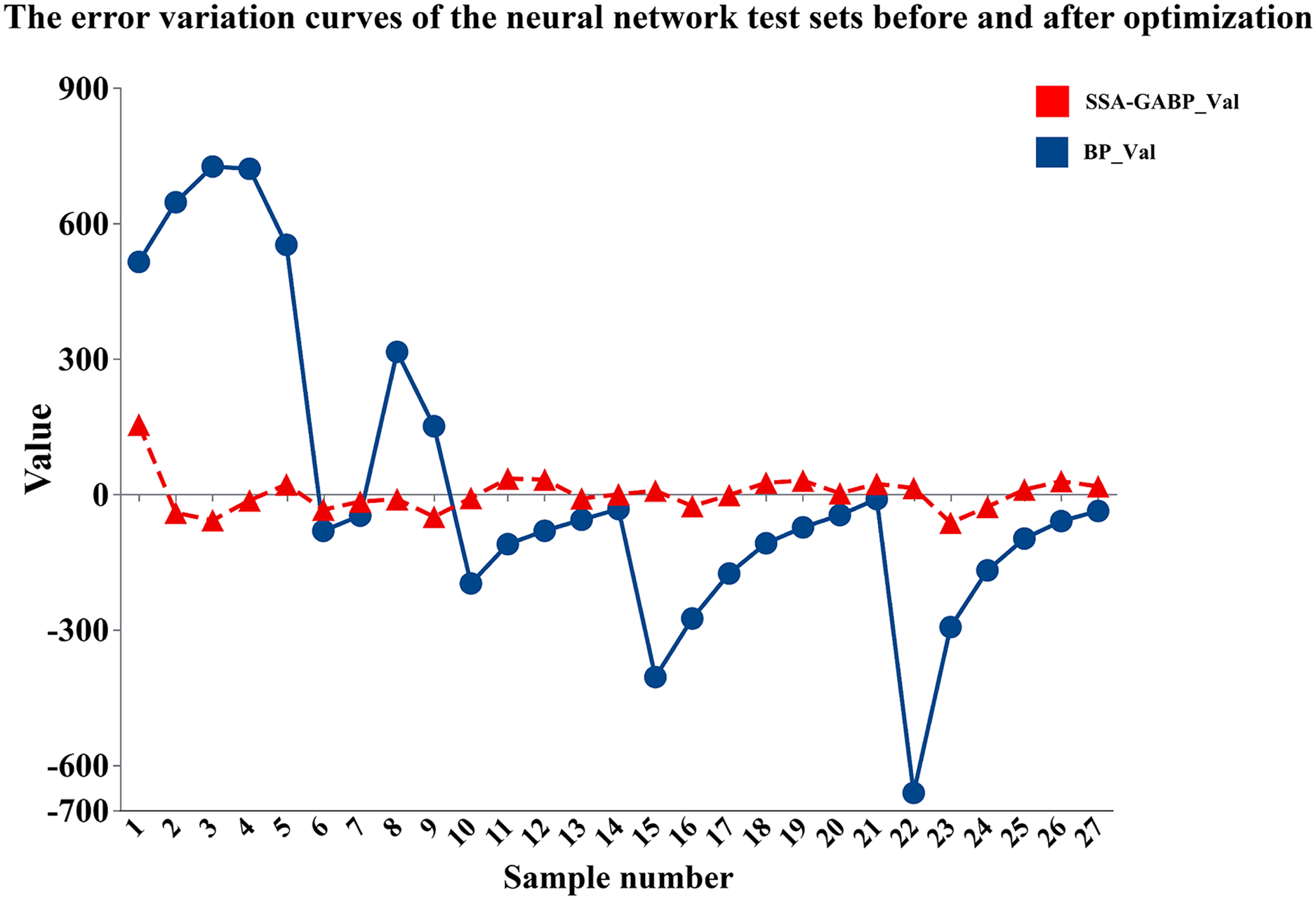
Figure 16: Comparison of neural network error curves

4  Box-Behnken Response Surface Analysis

The principle of regression fitting of data by neural networks is to find the bias and weight of the hidden layer, which implicitly expresses the input and output relationship of the data through multiple expressions. However, when using the rate-temperature-viscosity constitutive model of a certain propellant, an exact function expression is needed to represent it. This paper proposes to use the trained network and Box-Behnken response surface simulation to fit a functional analytical formula that can reflect the constitutive model of the viscosity of a certain propellant. Experimental design is carried out using Box-Behnken, and 17 groups of design experiments are constructed.

Take the samples of the experimental design as input, and use the trained network to perform regression fitting on them. The output of the grid training is taken as the response of the experimental design and filled in the table, as shown in the Table 3.

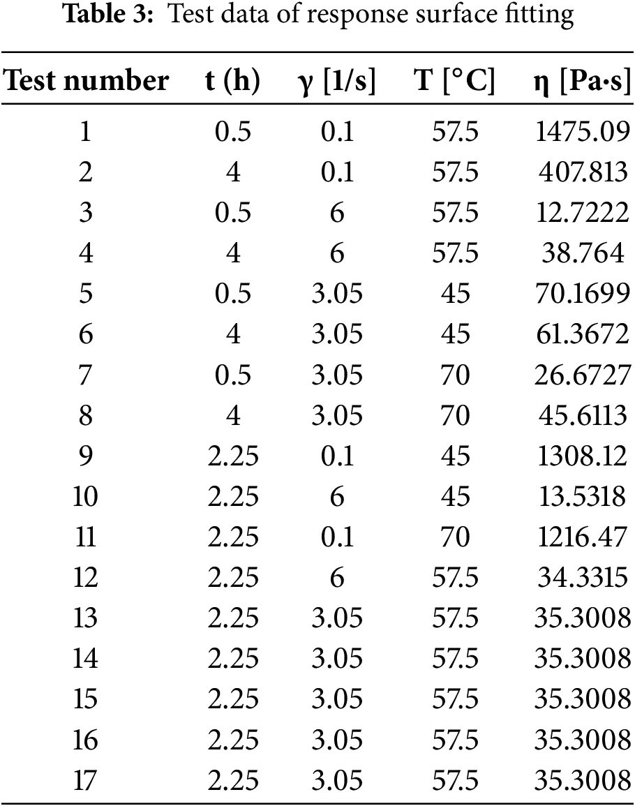
Then, response surface analysis was conducted on the input and response of the experimental design, and the R2 value of the fitted response surface was obtained to be 0.9477, which has a relatively high fitting accuracy. The 3D surfure diagram of the response surface fitting is shown in Fig. 17.

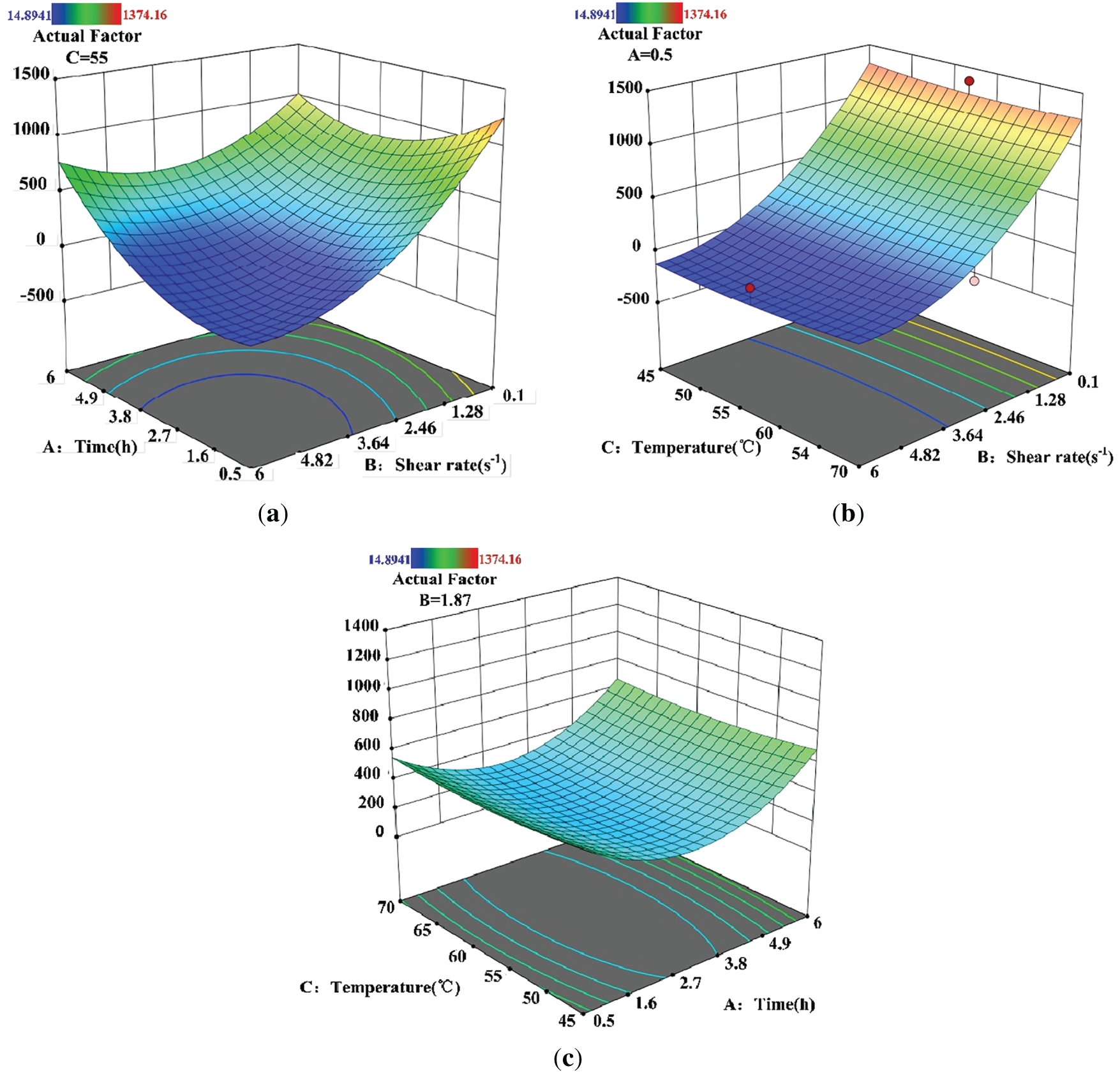
Figure 17: (a) Response surface curves of shear rate and temperature; (b) Response surface curves of shear rate and time; (c) Response surface curves of time and temperature

The Fig. 17 shows that the shear rate has a significant impact on the kinematic viscosity of a certain propellant, which conforms to the flow properties of non-Newtonian fluids, that is, the faster the shear rate, the greater the characteristic viscosity of the fluid. Box-Behnken response surface simulation was conducted for fluid viscosity, and regression fitting was performed on the input data.

Experimental data show that the shear rate (γ.) has a significant influence on the kinematic viscosity (η) of the propellant. From 0.1 to 6 s−¹, η decreased from 1475.09 to 12.72 Pa·s, presenting a shear thinning phenomenon. This trend conforms to the typical characteristics of non-Newtonian fluids. Box-Behnken response surface simulation was conducted for fluid viscosity, and regression fitting was performed on the input data.

According to the experimental design, taking the viscosity of the propellant as the objective function, the response surface approximation function was obtained by analyzing these 17 sample points using the least square method:

R1=2448.30653−320.56243at−544.04703g−32.54338ct+35.34456at∙bg−0.002285at∙ct+0.635354bg∙ct+42.23695at2+41.62045bg2+0.263439ct2(12)

In the formula: at represents the time after premixing; bg stands for shear rate; ct stands for temperature. Analysis of the fit and variance of the response model function. After obtaining the response surface, it is necessary to verify the degree of fitting. Usually, the F-test in statistics is used to conduct significance tests on the response surface model, and in engineering, its coefficient of determination is used to verify the degree of fitting of the response surface.

R2=∑i=1M(yi~−y~)2(yi−y−)2(13)

In the formula: yi—The mean response of the i-th sample; M—The number of sampling points designed; N—The number of basis functions of the response surface model.

By analyzing the response surface model, yields Y = 0.9447, which approaches 1, indicating a relatively high fitting accuracy and meeting the accuracy requirements. The R2 fitting curve is shown in the Fig. 18.

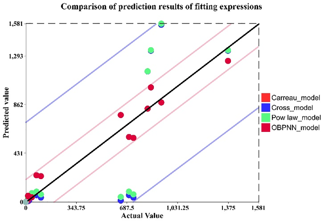
Figure 18: Comparison of prediction results offitting expressions

In this study, based on the experimentally determined viscosity data of the propellant, we first conducted parameter fitting for three classical constitutive models (power-law, Cross, Carreau) and a neural network-response surface composite model, respectively. Subsequently, the predicted viscosity values of each model were plotted on the same scatter plot with the actual experimental values, and a 45° reference line was introduced to visually compare the prediction accuracy. It can be seen that all the prediction points of the neural network—response surface model are almost linearly distributed along the 45° reference line, and the deviation between them and the true values is extremely small, reflecting that this method has a significant advantage in fitting accuracy. The prediction points of the traditional constitutive model deviate significantly from the 45° reference line, and the error shows a systematic distribution. Especially in the high shear rate or high temperature sections, the residual is more concentrated, indicating that simple power laws or empirical formulas are difficult to describe the complex rheological behavior of propellants. This result further verifies that in the rheological study of propellants with multi-factor coupling and significant nonlinearity, simple empirical constitutive equations are difficult to achieve accuracy under various working conditions. By combining neural networks with response surface methods, not only can the high-order interaction effects of shear rate, temperature and time be captured, but also the prediction reliability can be significantly improved.

The performance of different models can be more intuitively seen from Fig. 19. It is obvious that the Root Mean Squared Error (RMES) of the model established in this paper is 101.06, which is the smallest among all the models, indicating that the model is superior to the traditional model in viscosity prediction.

Figure 19: Comparison of RMSE across models

5  Conclusion

Based on the experimental-measured non-Newtonian rheological data of a certain type of solid rocket propellant slurry under multiple working conditions (shear rate, premixing time, temperature), We conducted research on the characterization and prediction methods of solid propellant slurry through model comparison and method integration. The main conclusions are as follows:

(1)   Under the unified data and evaluation criteria, SVM, RF and BPNN were compared. Although the nonlinear fitting ability of the traditional BPNN is superior to that of SVM and RF, its overall accuracy and robustness are still insufficient to meet the requirements of engineering simulation, especially with relatively large errors in the high shear rate and high-temperature sections.

(2)   To improve the performance of the model, a BP model (SSA-GA-BP) with the collaborative optimization of SSA and GA is proposed. By conducting dual optimization of the initial weights and thresholds of the network, the global optimization and local convergence capabilities are significantly enhanced. The results show that the coefficient of determination of SSA-GA-BP increases from R2 = 0.413 to R2 = 0.948, the prediction variance increases by 108%, and RMSE decreases significantly. Within the key pouring viscosity range (200–600 Pa·s), the prediction point closely adheres to the 45° reference line, demonstrating higher reliability.

(3)   Relying on the SSA-GA-BP output, the Box-Behnken response surface is adopted to fit the three factors of shear rate, temperature and time into an explicit quadratic polynomial constitutive, achieving the parsing and CFD-friendly embedding of the “black Box” mapping of neural networks, while taking into account both interpretability and computational efficiency. This explicit constitutive model can be directly embedded into CFD simulations to optimize process parameters, reduce casting defects such as voids and cracks, and improve mold-filling quality. Furthermore, by ensuring accurate viscosity prediction within the critical range, the proposed method supports batch-to-batch consistency, enhances the reliability of the propellant column structure, and provides quantitative rheological parameters for subsequent structural analysis and optimization of solid rocket motors.

While the present results are encouraging, they were derived under a single-formulation dataset and specific operating ranges; broadening data sources, adding cross-site validation and uncertainty quantification, and exploring surrogates beyond quadratic forms would be valuable directions to further strengthen generalization and CFD applicability.

Acknowledgement: Thanks for the support of the National Natural Science Foundation of China and the cooperative enterprise Inner Mongolia Aerospace Hongxia Chemical Co., Ltd.

Funding Statement: This research was funded by the National Natural Science Foundation of China (Grant No. 51965048). The funding facilitated access to specialized laboratory equipment, covered essential consumables for experiments, and provided partial support for graduate student assistants involved in data acquisition and preliminary analysis.

Author Contributions: The authors confirm contribution to the paper as follows: study conception and design: Zhaoxia Cui (corresponding author), Minghai Zheng; data collection: Minghai Zheng, Jiang Liu; analysis and interpretation of results: Minghai Zheng, Jianjun Li; draft manuscript preparation: Minghai Zheng; supervision/project administration: Zhaoxia Cui. All authors reviewed the results and approved the final version of the manuscript.

Availability of Data and Materials: The data that support the findings of this study are available from the Corresponding Author [Zhaoxia Cui].

Ethics Approval: Not applicable.

Conflicts of Interest: The authors declare no conflicts of interest to report regarding the present study.

References

1. Du X, Liu J, Chen J, Wang F, Deng H, Wang P, et al. Butyl hydroxy propellant rheology research. J Explos Fire. 2023;46(11):1007–13. (In Chinese). doi:10.14077/j.iSSN.1007-7812.202303035. [Google Scholar] [CrossRef]

2. Yue X, Wu Y, Li K. Experimental study and numerical simulation of viscosity measurement of solid propellant slurry by press bar-fall ball viscometer. Propellants Explos Pyrotech. 2021;46(4):663–9. doi:10.1002/prep.202000286. [Google Scholar] [CrossRef]

3. Hoque E, Ghosal S, Nagar N, Patil RS. Rheo-kinetic study of 4-(Dimethylsilyl) butyl ferrocene-grafted HTPB-based composite propellant and evaluation of casting rate. Asia-Pac J Chem Eng. 2023;18(5):e2960. doi:10.1002/apj.2960. [Google Scholar] [CrossRef]

4. Yue W, Zhuo L, Rong L. Solid propellant plate casting: numerical simulation and experimental study. J Fire Explosives. 2018;9(5):506–11. doi:10.14077/j.issn.1007-7812.2018.05.015. [Google Scholar] [CrossRef]

5. Wang H, Zhi S, Cao J, Qiang H. Influence of solid propellant slurry leveling on integrity of engine charge structure. Solid Rocket Technol. 2019;42(3):345–50. (In Chinese). [Google Scholar]

6. Wang Z, Qiang H. Mechanical properties of thermal aged HTPB composite solid propellant under confining pressure. Defence Technol. 2022;18(4):618–25. doi:10.1016/j.dt.2021.06.014. [Google Scholar] [CrossRef]

7. Yuan S, Zhao Y, Luo Y. Rheological properties of HTPE/PCL four-component propellant slurry. J Fire Explosives. 2021;44(3):301–7. doi:10.14077/j.issn.1007-7812.202012009. [Google Scholar] [CrossRef]

8. Zhou J, Li Z, Lu R, Wei L, Zhang F. Experimental and simulation study on flow leveling of hydroxyl-terminated polybutadiene propellant slurry. Polym Mater Sci Eng. 2023;33(6):85–92. doi:10.16865/j.cnki.1000-7555.2023.0081. [Google Scholar] [CrossRef]

9. Lu Y, Zhai G, Zhai W. Quantifying urban spatial resilience using multi-criteria decision analysis (MCDA) and back propagation neural network (BPNN). Int J Disaster Risk Reduct. 2024;111(2):104694. doi:10.1016/j.ijdrr.2024.104694. [Google Scholar] [CrossRef]

10. Meng D, Yang S, De Jesus AM, Zhu SP. A novel Kriging-model-assisted reliability-based multidisciplinary design optimization strategy and its application in the offshore wind turbine tower. Renew Energy. 2023;203:407–20. doi:10.1016/j.renene.2022.12.062. [Google Scholar] [CrossRef]

11. Liu X, Liu Z, Huang Z, Ling M, Lin K, Chen P, et al. Ergonomic reliability assessment of VDT system for operation design based on improved BPNN and HCR under special circumstances. Comput Model Eng Sci. 2023;136(1):685–707. doi:10.32604/cmes.2023.025058. [Google Scholar] [CrossRef]

12. Sun L, Wang Z, Cui S, Yan Z, Hu W, Meng Q. A novel model for describing rail weld irregularities and predicting wheel-rail forces using a machine learning approach. Comput Model Eng Sci. 2025;142(1):555–77. doi:10.32604/cmes.2024.056023. [Google Scholar] [CrossRef]

13. Meng D, Yang H, Yang S, Zhang Y, De Jesus AM, Correia J, et al. Kriging-assisted hybrid reliability design and optimization of offshore wind turbine support structure based on a portfolio allocation strategy. Ocean Eng. 2024;295:116842. doi:10.1016/j.oceaneng.2024.116842. [Google Scholar] [CrossRef]

14. Li M, Liu Z, Song H. An improved algorithm optimization algorithm based on RungeKutta and golden sine strategy. Expert Syst Appl. 2024;247:123262. doi:10.1016/j.eswa.2024.123262. [Google Scholar] [CrossRef]

15. Chen X, Liang C, Huang D, Real E, Wang K, Pham H, et al. Symbolic discovery of optimization algorithms. Adv Neural Inf Process Syst. 2023;36:49205–33. [Google Scholar]

16. Tian Z, Zhi P, Guan Y, Feng J, Zhao Y. An effective single loop Kriging surrogate method combing sequential stratified sampling for structural time-dependent reliability analysis. Structures. 2023;53:1215–24. doi:10.1016/j.istruc.2023.05.022. [Google Scholar] [CrossRef]

17. Zhu D, Wang S, Zhou C, Yan S, Xue J. Human memory optimization algorithm: a memory-inspired optimizer for global optimization problems. Expert Syst Appl. 2024;237:121597. doi:10.1016/j.eswa.2023.121597. [Google Scholar] [CrossRef]

18. Yang S, Wang H, Xu Y, Guo Y, Pan L, Zhang J, et al. A coupled simulated annealing and particle swarm optimization reliability-based design optimization strategy under hybrid uncertainties. Mathematics. 2023;11(23):4790. doi:10.3390/math11234790. [Google Scholar] [CrossRef]

19. Fattahi H, Ghaedi H, Armaghani DJ. Optimizing fracture toughness estimation for rock structures: a soft computing approach with GWO and IWO algorithms. Measurement. 2024;238:115306. doi:10.1016/j.measurement.2024.115306. [Google Scholar] [CrossRef]

20. Yang H, Yang S, Meng D, Hu C, Wu C, Yang B, et al. Optimization of analog circuit parameters using bidirectional long short-term memory coupled with an enhanced whale optimization algorithm. Mathematics. 2025;13(1):121. doi:10.3390/math13010121. [Google Scholar] [CrossRef]

21. Xiao M, Luo R, Chen Y, Ge X. Prediction model of asphalt pavement functional and structural performance using PSO-BPNN algorithm. Constr Build Mater. 2023;407(1):133534. doi:10.1016/j.conbuildmat.2023.133534. [Google Scholar] [CrossRef]

22. Lin Q, Yang S, Yang R, Wu H. Transistor modeling based on LM-BPNN and CG-BPNN for the GaAs pHEMT. Int J Numer Model Electron Netw Devices Fields. 2024;37(4):e3268. doi:10.1002/jnm.3268. [Google Scholar] [CrossRef]

23. Xie J, Tian Z, Zhi P, Zhao Y. Reliability analysis method of coupling optimal importance sampling density and multi-fidelity Kriging model. Eksploat I Niezawodn-Maint Reliab. 2023;25(2):161893. doi:10.17531/ein/161893. [Google Scholar] [CrossRef]

24. Rao D, Huang M, Shi X, Yu Z, He Z. A microseismic signal denoising algorithm combining VMD and wavelet threshold denoising optimized by BWOA. Comput Model Eng Sci. 2024;141(1):187–217. doi:10.32604/cmes.2024.051402. [Google Scholar] [CrossRef]

25. Xue J, Shen B. A novel swarm intelligence optimization approach: sparrow search algorithm. Syst Sci Control Eng. 2020;8(1):22–34. doi:10.1080/21642583.2019.1708830. [Google Scholar] [CrossRef]

26. Ye Z, Wang JG, Yang J. A multi-objective optimization approach for a fault geothermal system based on response surface method. Geothermics. 2024;117:102887. doi:10.1016/j.geothermics.2023.102887. [Google Scholar] [CrossRef]

27. Zhan Y, Zhu J. Response surface methodology and artificial neural network-genetic algorithm for modeling and optimization of bioenergy production from biochar-improved anaerobic digestion. Appl Energy. 2024;355:122336. doi:10.1016/j.apenergy.2023.122336. [Google Scholar] [CrossRef]

28. Meng D, Yang S, De Jesus AM, Fazeres-Ferradosa T, Zhu SP. A novel hybrid adaptive Kriging and water cycle algorithm for reliability-based design and optimization strategy: application in offshore wind turbine monopile. Comput Methods Appl Mech Eng. 2023;412:116083. doi:10.1016/j.cma.2023.116083. [Google Scholar] [CrossRef]

29. Li JY, Zhan ZH, Zhang J. Evolutionary computation for expensive optimization: a survey. Mach Intell Res. 2022;19(1):3–23. doi:10.1007/s11633-022-1317-4. [Google Scholar] [CrossRef]

30. Song Z, Wang H, He C, Jin Y. A kriging-assisted two-archive evolutionary algorithm for expensive many-objective optimization. IEEE Trans Evol Comput. 2021;25(6):1013–27. doi:10.1109/tevc.2021.3073648. [Google Scholar] [CrossRef]

31. Meng D, Li Y, He C, Guo J, Lv Z, Wu P. Multidisciplinary design for structural integrity using a collaborative optimization method based on adaptive surrogate modelling. Mater Des. 2021;206:109789. doi:10.1016/j.matdes.2021.109789. [Google Scholar] [CrossRef]

32. Buscema M. Back propagation neural networks. Subst Use Misuse. 1998;33(2):233–70. doi:10.3109/10826089809115863. [Google Scholar] [PubMed] [CrossRef]

33. Lei H. Solid rocket propellant inserted-core forming porosity control method research [dissertation]. Hohhot, China: Inner Mongolia University of Technology; 2021. (In Chinese). doi:10.27225/d.cnki.gnmgu.2021.000061. [Google Scholar] [CrossRef]