Shock-Boundary Layer Interaction in Transonic Flows: Evaluation of Grid Resolution and Turbulence Modeling Effects on Numerical Predictions

1  Introduction

Transonic flow simulation remains one of the most challenging areas in computational fluid dynamics (CFD) due to the complex physics involved, particularly the shock wave/boundary layer interactions. These interactions are critical in determining the aerodynamic performance of various aerospace applications, from aircraft wings to turbomachinery components [1,2]. The accurate prediction of such flows is therefore essential for efficient design optimization and performance assessment.

A significant body of research has focused on mesh resolution as a key factor in improving the accuracy of transonic flow simulations. High-resolution meshes are essential for accurately resolving intricate flow features, particularly in regions where shock waves are present. Widiawaty et al. [3] emphasized that mesh resolution plays a crucial role in CFD, directly impacting result accuracy, and highlighted the necessity of refining meshes in critical flow regions. Kulkarni et al. [4] demonstrated that the choice of mesh significantly influences flow characteristics and turbulence model performance, finding that coarser meshes failed to accurately capture shock positions. Hashimoto et al. [5] investigated unsteady transonic buffet and reported that accurate prediction of shock location remains challenging even with fine grids unless appropriate wall modeling is used.

The selection of turbulence models represents another decisive factor for the accurate simulation of transonic flows. Different models exhibit varying capabilities in capturing the complexities of transonic phenomena. The Spalart-Allmaras (SA) and k-ω Shear Stress Transport (SST) models are commonly employed due to their robustness in handling transonic conditions [6,7]. Duggirala et al. [6] compared these models for predicting interference drag in transonic flows and found significant variations in predicted drag values depending on model choice, with differences up to 30% in some configurations. Yi et al. [8] demonstrated that turbulence model selection affects flow prediction accuracy in transonic flows, with k-ω models generally performing better near separation regions. Soda [9] conducted numerical investigations of 2D and 3D unsteady transonic flows using hybrid Reynolds-Averaged Navier-Stokes/Detached Eddy Simulation (RANS/DES) approaches and found that shock buffet predictions were highly sensitive to turbulence modeling parameters. Petrocchi and Barakos [10] assessed the Partially Averaged Navier-Stokes (PANS) method for transonic buffet simulations and found it superior to Unsteady Reynolds-Averaged Navier-Stokes (URANS) in resolving flow unsteadiness on affordable grids. Nevertheless, standard RANS models have been shown to often struggle in accurately modeling shock-boundary layer interactions [7,11].

The interaction between mesh resolution and turbulence modeling has also been explored in several contexts. Galpin et al. [12] validated CFD simulations against experimental data from a transonic axial compressor, assessing sensitivity to mesh size, turbulence models, and other factors, and showed that accurate prediction of shock-boundary layer interactions required both appropriate turbulence modeling and sufficient mesh resolution. Hosangadi et al. [13] presented simulations for transonic diffuser-volute configurations using unstructured CFD and achieved good agreement with experimental data by employing multi-element unstructured frameworks that provided better resolution around critical geometry features. Coratger et al. [14] developed a hybrid lattice-Boltzmann method for complex transonic flows that combined grid refinement with subgrid turbulence models, demonstrating good predictive capability.

In parallel, machine learning approaches have recently emerged as promising tools for transonic flow prediction. Zhou et al. [15] developed a deep learning framework using residual networks that accurately captured essential physical features such as shock strength, location, flow separation, and boundary layer characteristics in transonic regimes. Jia et al. [16] created a hybrid method fusing deep learning with reduced-order modeling that reduced prediction errors in nonlinear flow regions by 13%–66%, while maintaining computational efficiency. Complementary to these developments, Mufti et al. [17] proposed a domain-informed probabilistic deep learning framework for predicting transonic flow fields, achieving 6.4% error in shock strength and 1% error in shock location prediction, and outperforming traditional reduced-order models by 60%. Al-Rbaihat et al. [18] combined RANS/DES-based CFD with Gaussian process regression (GPR) to demonstrate the effectiveness of hybrid CFD-Machine Learning (CFD-ML) methodologies in handling complex shock-dominated flows.

Despite these advances in transonic flow simulation, the review of the literature reveals a gap: there is a notable absence of comprehensive studies that systematically investigate the combined effects of mesh resolution and turbulence model selection. Most prior work has either optimized mesh resolution with a fixed turbulence model or compared turbulence models on a single mesh, with little attention to how steady and unsteady solvers behave under these combined conditions. This fragmented approach overlooks key interdependencies that directly influence prediction accuracy. In particular, the interaction between different non-dimensional wall distance (y+) values and turbulence models has not been thoroughly explored for transonic airfoils, even though this is critical for accurately capturing shock-boundary layer interactions. The complex interactions between shock waves and boundary layers in transonic flows make this combined analysis especially important, as turbulence model performance can vary depending on near-wall mesh resolution. This study investigates the combined effects of mesh resolution and turbulence model selection on transonic flow predictions. By comparing different y+ values implemented with both moderate and fine mesh resolutions and evaluating three widely used turbulence models with both steady and unsteady solvers, this research provides a comprehensive assessment of how these factors interact to affect transonic simulation accuracy and shock prediction. The novelty of this work lies in its systematic integration of mesh sensitivity, including near-wall y+ resolution, with turbulence model selection in a unified transonic airfoil framework. Furthermore, by explicitly contrasting steady and unsteady solvers, the study delivers practical guidelines in selecting appropriate modeling strategies under varying computational resource constraints.

2  Materials and Methods

2.1 RAE2822 Data Airfoil and Experimental Data

The experimental dataset for this study is taken from the Advisory Group for Aerospace Research and Development (AGARD) AR-138 report on the RAE2822 airfoil [19]. Case 13A was selected, corresponding to a Mach number of 0.74, a Reynolds number of 2.7 × 106, and an angle of attack of 3.19∘. The available experimental measurements include surface pressure coefficient distributions as well as integrated aerodynamic coefficients. These data are widely used as a benchmark for assessing the accuracy of computational methods in transonic flow regimes.

2.2 Computational Domain and Mesh Generation

The computational domain employs a C-grid topology surrounding the RAE2822 airfoil, extending 20 chord lengths in all directions to minimize far-field boundary effects. The mesh was generated using OpenFOAM’s native blockMesh utility, with the blockMesh dictionary was configured to enhance cell distribution, particularly near the shock region for accurate boundary layer resolution. The first cell height was calculated to achieve target y+ values of 1, 2.5, and 5. These correspond to 1 × 10−5c, 2.5 × 10−5c, and 5 × 10−5c, where c represents the chord length. A growth rate of 1.2 was employed from the airfoil surface outward. Mesh quality was verified using OpenFOAM’s checkMesh utility. All grids have max. skewness and orthogonal quality values around 0.8 and 40 respectively. As detailed in Table 1, the study utilized six distinct hexahedral mesh configurations: M1 and M2 (max. y+≈1), M3 and M4 (max. y+≈2.5), and M5 and M6 (max. y+≈5), where M2, M4, and M6 represent globally higher-density versions of M1, M3, and M5, respectively.

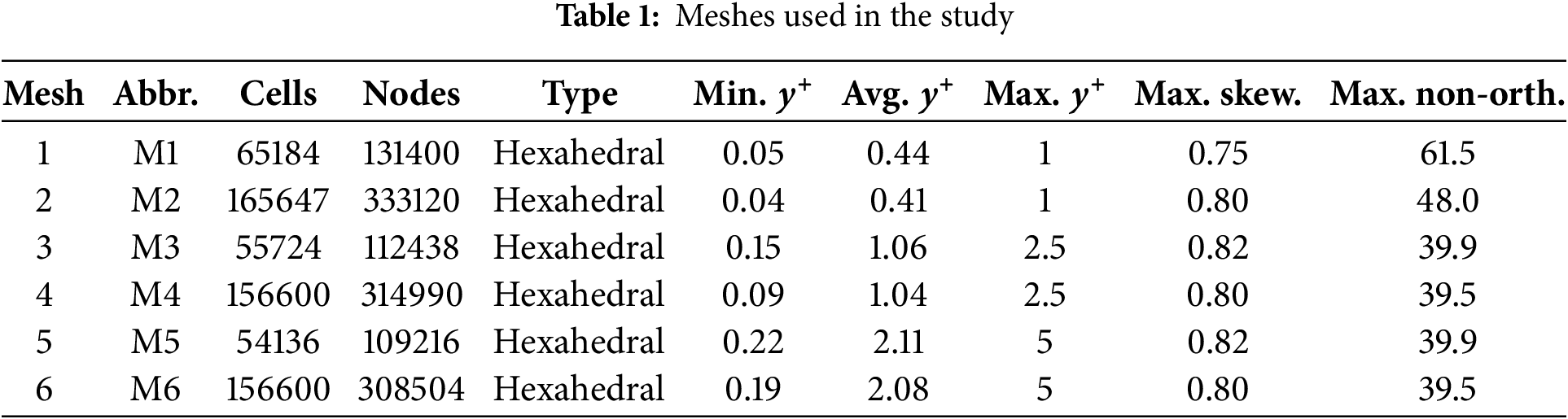
Fig. 1 presents the representative mesh pairs, showing (a) the complete domain configuration of the fine grid, with close-up views comparing (b) moderate and (c) fine resolutions. This systematic approach of varying both near-wall resolution (y+) and global mesh density enables evaluation of grid sensitivity on flow solution accuracy. Fine meshes contain approximately 2.5–2.9 times more cells than their moderate counterparts, yet the overall mesh quality metrics remain nearly unchanged. The baseline mesh properties were selected considering previous RAE2822 studies in the literature [20–24]. On the airfoil surface, the moderate meshes include approximately 220 grid cells, while the fine meshes include about 420 grid cells. The simulations were run on quasi-2D meshes, with a single cell used in the spanwise direction.

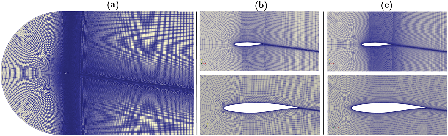
Figure 1: Computational mesh visualization: (a) Complete domain view of the fine-resolution C-grid configuration (M2); (b) Close-up views from the moderate-resolution mesh (M1); (c) Close-up views from the fine-resolution mesh (M2)

2.3 Numerical Solvers

Two solvers are used for steady and unsteady simulations: TSLAerofoam and rhoCentralFoam, both based on the OpenFOAM framework.

The rhoCentralFoam is an unsteady density-based solver for high-speed compressible flow included in the standard OpenFOAM distribution. As described by Greenshields et al. [25], this solver implements a semi-discrete, non-staggered central scheme developed by Kurganov and Tadmor [26]. The CFD solver discretizes the continuity, momentum, and energy equations separately to obtain three linear systems [27].

∂ρ∂t+∇⋅(Uρ)=0(1)

∂(ρU)∂t+∇⋅[U(ρU)]+∇p+∇⋅σ=0(2)

∂(ρE)∂t+∇⋅[U(ρE)]+∇⋅(Up)+∇⋅(σ⋅U)+∇⋅j=0(3)

where ρ is density, U is velocity, p is pressure, and E is total energy given by E=e+|U|2/2, with e representing the specific internal energy or enthalpy. The viscous stress tensor σ is defined as positive in compression:

σ = −μ[∇U+(∇U)T−23(∇⋅U)I].(4)

with dynamic viscosity μ, unit tensor I, and diffusive heat flux j defined by Fourier’s law with thermal conductivity kth and temperature T:

j = −kth∇T.(5)

This central-upwind scheme offers an alternative approach to traditional Riemann solvers, combining central-difference and upwind schemes, making it particularly effective for flows with shocks and discontinuities in transonic regimes [28,29].

The second solver, TSLAeroFoam, is a steady-state, density-based compressible flow solver developed within the OpenFOAM-based NextFOAM framework. It employs the Lower–Upper Symmetric Gauss–Seidel (LU-SGS) algorithm for implicit time integration, which enables rapid convergence for steady computations. Tailored for aerospace applications, the solver incorporates Riemann-based boundary conditions, advanced near-wall treatment, and the thin shear layer (TSL) approximation, which improves efficiency in boundary layer-dominated transonic flows. In TSLAeroFoam, convective fluxes are computed using the Roe-FDS (flux difference splitting) scheme with VK-limited gradient reconstruction, while viscous fluxes are modeled with the TSL approximation. A second-order upwind scheme is consistently applied to both convective and turbulence terms [30,31].

The use of both steady and unsteady solvers allows a direct comparison in transonic simulations. The rhoCentralFoam enables the capture of possible transient effects associated with shock-boundary layer interaction in transonic conditions, while TSLAeroFoam provides an efficient steady-state baseline. This setup makes it possible to assess how mesh resolution and turbulence modeling influence solution accuracy differently in steady vs. unsteady frameworks.

2.4 Numerical Simulations

A comprehensive matrix of simulations was performed to systematically investigate the effects of mesh resolution, y+ values, and turbulence models on the prediction accuracy of transonic flow phenomena. All simulations were conducted at the specified flow conditions of M = 0.74, Re = 2.7 × 106, and α = 3.19∘. The air was modeled as a perfect gas. The following turbulence models were evaluated.

•   Spalart-Allmaras (SA)—A one-equation model known for its robustness in aerospace applications [32].

Dν~Dt=Cb1(1−ft2)S~ν~+1σ[∇⋅((ν+ν~)∇ν~)+Cb2|∇ν~|2]−[Cw1fw−Cb1κ2ft2](ν~d)2(6)

Here, ν~ is the working variable related to eddy viscosity, ν is the molecular viscosity, d is the wall distance, S~ is a modified vorticity magnitude, and Cb1,Cb2,Cw1,σ,κ are model constants.

•   k-ω SST—A two-equation model that combines the advantages of k-ω in the near-wall region and k-ϵ in the free stream [33,34].

∂(ρk)∂t+∇⋅(ρkU)=Pk−β∗ρkω+∇⋅[(μ+σkμt)∇k](7)

∂(ρω)∂t+∇⋅(ρωU)=αωkPk−βρω2+∇⋅[(μ+σωμt)∇ω]+2(1−F1)ρσω2ω∇k⋅∇ω(8)

Here, k is the turbulent kinetic energy, ω is the specific dissipation rate, Pk is the production term, μt is the eddy viscosity, μ is the molecular viscosity, ρ is density, and α,β,β∗,σk,σω,σω2 are model constants.

•   k-ϵ Realizable—A two-equation model with enhanced treatment of the dissipation rate equation [35,36].

∂(ρk)∂t+∇⋅(ρkU)=∇⋅[(μ+μtσk)∇k]+Pk−ρϵ(9)

∂(ρϵ)∂t+∇⋅(ρϵU)=∇⋅[(μ+μtσϵ)∇ϵ]+ρC1Sϵ−ρC2ϵ2k+νϵ(10)

Here, k is turbulent kinetic energy, ϵ is the dissipation rate of k, Pk is the production of k, S=2SijSij is the mean strain rate magnitude, μt is the eddy viscosity, ν is the molecular kinematic viscosity. C1=max[0.43,η/(η+5)] where η=Sk/ϵ is a variable coefficient, while C2,σk,σϵ are model constants.

The unsteady simulations were performed using the rhoCentralFoam solver of OpenFOAM v2406. The maximum Courant number was set to 0.7, resulting in time step sizes of 2.6 × 10−8 s for M1 and M2, 6.5 × 10−8 s for M3 and M4, and 1.3 × 10−7 s for M5 and M6. Key numerical settings and parameters are presented in Table 2. Fig. 2 illustrates the overall research workflow, from mesh generation through solver and turbulence-model selection to simulations, post-processing, and final comparisons. The unsteady simulations were run for approximately 0.25 s in real flow time, which corresponds to nearly two flow-through periods of the computational domain. For the unsteady simulations, the final aerodynamic coefficients, lift, drag, and moment (CL,CD, and CM), were calculated by averaging the simulation data over the last 0.05 s. A representative convergence history for the M3 mesh configuration with the SA turbulence model is presented in Fig. 3a, showing the evolution of CL over time.

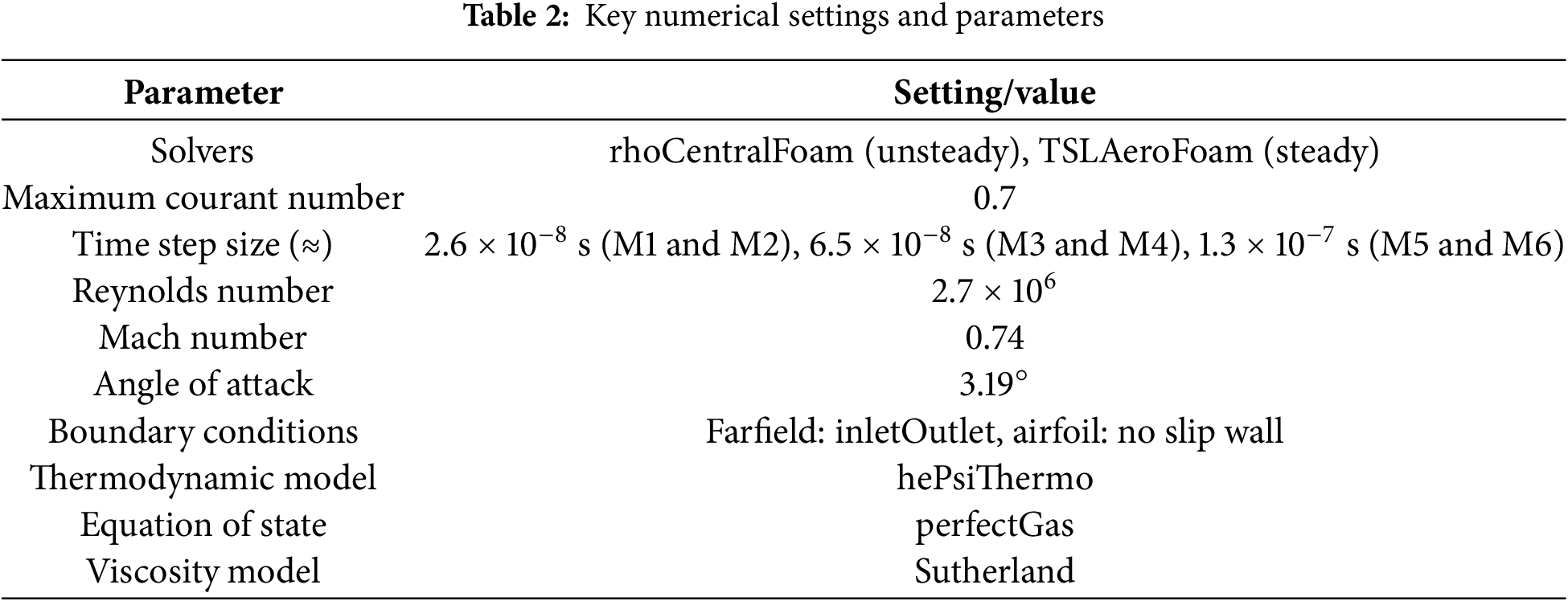
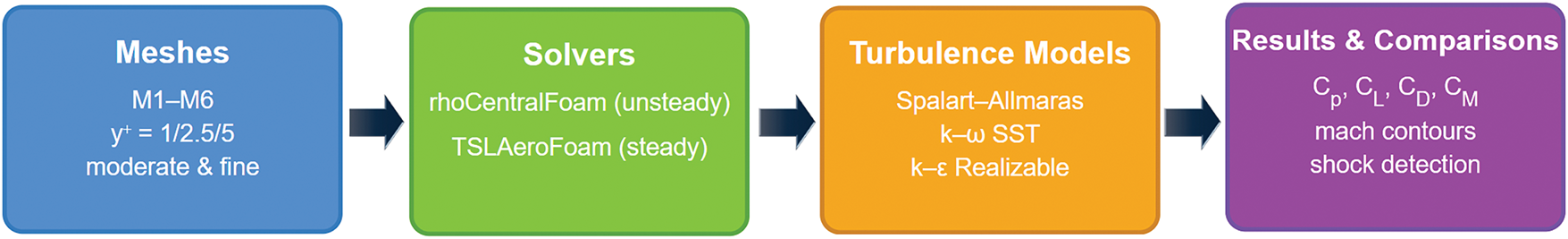
Figure 2: Flowchart of the research workflow

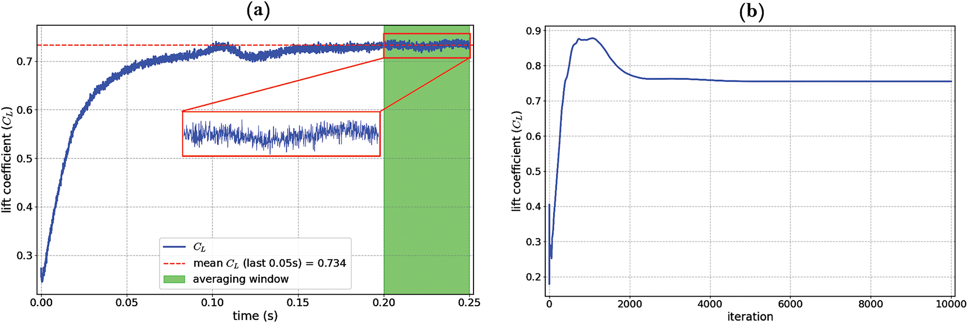
Figure 3: Representative convergence histories for the M3 mesh configuration: (a) CL vs. time from rhoCentralFoam, (b) CL vs. iteration from TSLAeroFoam

For the steady-state simulations with TSLAeroFoam, a maximum of 10,000 iterations was performed, and convergence was ensured by requiring all residuals to fall below 10−5, confirming the stability of the steady solutions. In addition, the evolution of CL with iteration was monitored to verify convergence, and a representative CL-iteration history is presented in Fig. 3b. The computational time for the steady cases was less than 30 min on 24 CPU cores (Intel E5 2650v3 CPU), whereas the unsteady rhoCentralFoam simulations required between one day and one week depending on mesh. The shock location was determined approximately as the point on the suction side where the pressure coefficient (−Cp) reached its maximum value and subsequently began to decrease. Both a steady and an unsteady solver were employed to allow direct comparison of results: the unsteady solver was able to capture possible transient effects associated with shock-boundary layer interaction at transonic conditions, while the steady solver provided an efficient baseline for routine aerodynamic prediction and highlighted the trade-off between accuracy and computational cost.

3  Results and Discussion

Fig. 4 compares rhoCentralFoam predictions with experimental data across turbulence models and mesh resolutions, revealing key findings about shock location sensitivity. While all models show some dependence on near-wall resolution, the k-ϵ Realizable model exhibits significantly greater sensitivity to increasing y+ values (from 1 to 5) compared to both Spalart-Allmaras and k-ω SST models. At y+=1, the shock locations predicted by the k-ω SST and SA models are very close to the experimental value (x/c≈0.50), with deviations of only 0%–2%, while the k-ϵ Realizable model shows larger errors up to 6%. As y+ increases to 5, the k-ϵ Realizable model displaces the shock by as much as 12%, whereas the k-ω SST retains errors typically below 2%. In terms of lift, rhoCentralFoam predicts CL within about 2% of the experimental value (CL=0.733), while TSLAeroFoam tends to overpredict by about 4%. The k-ω SST model demonstrates the most consistent performance, maintaining accurate shock location even at higher y+ values, albeit with a slight loss of sharpness in the pressure recovery region. This robustness is consistent with its established reputation in transonic flow studies [6,10]. Spalart-Allmaras also performs reasonably well but underestimates suction peaks in some cases, reflecting its simpler one-equation formulation. It should be noted that the unsteady solver introduces minor temporal oscillations in lift and shock position, which are a known characteristic of buffet-like unsteadiness in transonic airfoils. These oscillations, while small, highlight the influence of temporal resolution in capturing flow physics.

Figure 4: Comparison of CFD results obtained using different turbulence models with rhoCentralFoam on grids (a) M1, (b) M2, (c) M3, (d) M4, (e) M5, and (f) M6 against experimental data

Fig. 5 presents Mach number contours from the unsteady rhoCentralFoam solver across six mesh configurations and three turbulence models. The flow velocity reaches around M = 1.4 on the suction side and remains around M = 0.6 on the pressure side near the leading edge. When comparing the contours, two main trends can be observed. First, increasing global mesh density generally reduces the extent of low-Mach number regions while slightly expanding high-Mach zones. This effect is most evident near the shock formation area, where finer meshes yield more compact supersonic regions compared to their moderate-resolution counterparts. Second, reducing y+ from 5 to 1 produces a clear contraction of high-Mach zones, indicating better resolution of viscous effects near the airfoil surface. Among the tested models, the k-ω SST captures sharper leading-edge acceleration, maintains shock positions close to experimental observations, and produces smoother pressure recovery downstream of the shock. Spalart-Allmaras shows broadly similar behavior but with slightly smoother contours, while the k-ϵ Realizable model is more sensitive to y+ variations, with high-Mach regions shrinking more substantially at lower y+ levels, which may be linked to its limitations in adverse pressure gradient flows.

Figure 5: Mach number contours obtained from the rhoCentralFoam solver for six mesh configurations using three turbulence models: Spalart-Allmaras, k-ω SST, and k-ϵ Realizable

Fig. 6 displays Mach contours from the steady-state TSLAeroFoam solver, revealing several key differences from the unsteady results. The steady solver demonstrates significantly reduced sensitivity to both mesh density and y+ variations compared to rhoCentralFoam. Similar tendencies are still visible: increasing global mesh density expands the high-Mach regions and sharpens the shock definition, but the magnitude of these effects is reduced, especially near the shock. The contours exhibit marginally shallower gradients in the flow direction, suggesting that the steady approach produces somewhat smoother transitions between flow regimes. As with the unsteady case, increasing y+ values produce a modest growth in high-Mach regions, though this effect is less pronounced than observed in Fig. 5. The k-ω SST model again delivers the most consistent results across mesh variations, while Spalart-Allmaras shows better agreement with expected physical behavior in the steady formulation compared to its unsteady performance. Smoother shock representation of the steady solver is likely due to its inability to resolve transient buffet-like dynamics, which in practice reduces variability but can mask certain unsteady flow physics.

Figure 6: Mach number contours obtained from the TSLAeroFoam solver for all six mesh configurations using three turbulence models: Spalart-Allmaras, k-ω SST, and k-ϵ Realizable

Fig. 7 compares TSLAeroFoam’s steady-state pressure distributions with experimental data across six mesh configurations and three turbulence models, revealing several important insights. The k-ω SST model demonstrates superior performance in shock location prediction, capturing the experimental shock position within 0.01c (≈2%) on fine y+≈1 meshes (M1/M2), while Spalart-Allmaras shows comparable accuracy though with slight underprediction of the suction peak. The k-ϵ Realizable model consistently displaces shocks 0.01–0.04 c toward the trailing edge and overestimates post-shock pressures compared to experimental values. Increases in global mesh density are less pronounced in steady simulations than in the unsteady results, though finer meshes still improve shock definition. Increasing y+ from 1 to 5 causes all models to predict more diffuse shock structures, with the k-ϵ Realizable showing the greatest sensitivity. The steady solver’s sharper shock representation is linked to its tendency to overpredict suction-side −Cp levels compared to both rhoCentralFoam and experimental data. This overprediction steepens the suction peak and makes the shock transition appear sharper. Temporal averaging in steady RANS approaches suppress certain shock-boundary layer interaction dynamics as noted in previous studies [9]. The k-ω SST model maintains its advantage across all tested conditions, though its performance edge over Spalart-Allmaras narrows at y+≈1, suggesting both models remain viable options for steady transonic simulations when fine near-wall resolution is achievable.

Figure 7: Comparison of CFD results obtained using different turbulence models with TSLAeroFoam on grids (a) M1, (b) M2, (c) M3, (d) M4, (e) M5, and (f) M6 against experimental data

Fig. 8 presents a comparative visualization of pressure coefficient (Cp) contours from rhoCentralFoam (top two rows) and TSLAeroFoam (bottom two rows) solvers using the k-ω SST model across all mesh configurations. Both solvers yield similar shock locations and pressure recovery patterns regardless of mesh density or y+ variation, indicating that the k-ω SST model achieves mesh-converged solutions even at moderate resolutions. TSLAeroFoam produces slightly stronger suction-side pressure gradients and sharper localized peaks at the shock, while rhoCentralFoam shows smoother transitions. These differences remain small in magnitude but become visible when comparing the solver results side by side. Both approaches capture the main flow physics, but their different solution strategies cause small differences, particularly in regions of strong acceleration and shock-boundary layer interaction.

Figure 8: Pressure coefficient (Cp) contours obtained from the rhoCentralFoam (top two rows) and TSLAeroFoam (bottom two rows) solvers for six mesh configurations using the k-ω SST turbulence model. The first rows show the top view, while the second rows show the perspective view of the airfoil

Fig. 9 compares the pressure distribution results of rhoCentralFoam and TSLAeroFoam using the k-ω SST model on the fine mesh with the lowest y+, M2. Although the two solvers predict very similar shock positions around x/c≈0.5, clear differences appear in other regions of the airfoil. On the suction side between x/c=0 and 0.5, TSLAeroFoam predicts higher −Cp values than rhoCentralFoam. In contrast, from x/c=0.5 to 1.0, rhoCentralFoam produces slightly higher −Cp levels compared to TSLAeroFoam. Furthermore, the Cp distribution obtained from TSLAeroFoam is smoother than that of rhoCentralFoam, most likely due to rhoCentralFoam’s unsteady nature.

Figure 9: Comparison of pressure coefficient (−Cp) distributions predicted by rhoCentralFoam and TSLAeroFoam using the k-ω SST turbulence model on the M2 grid

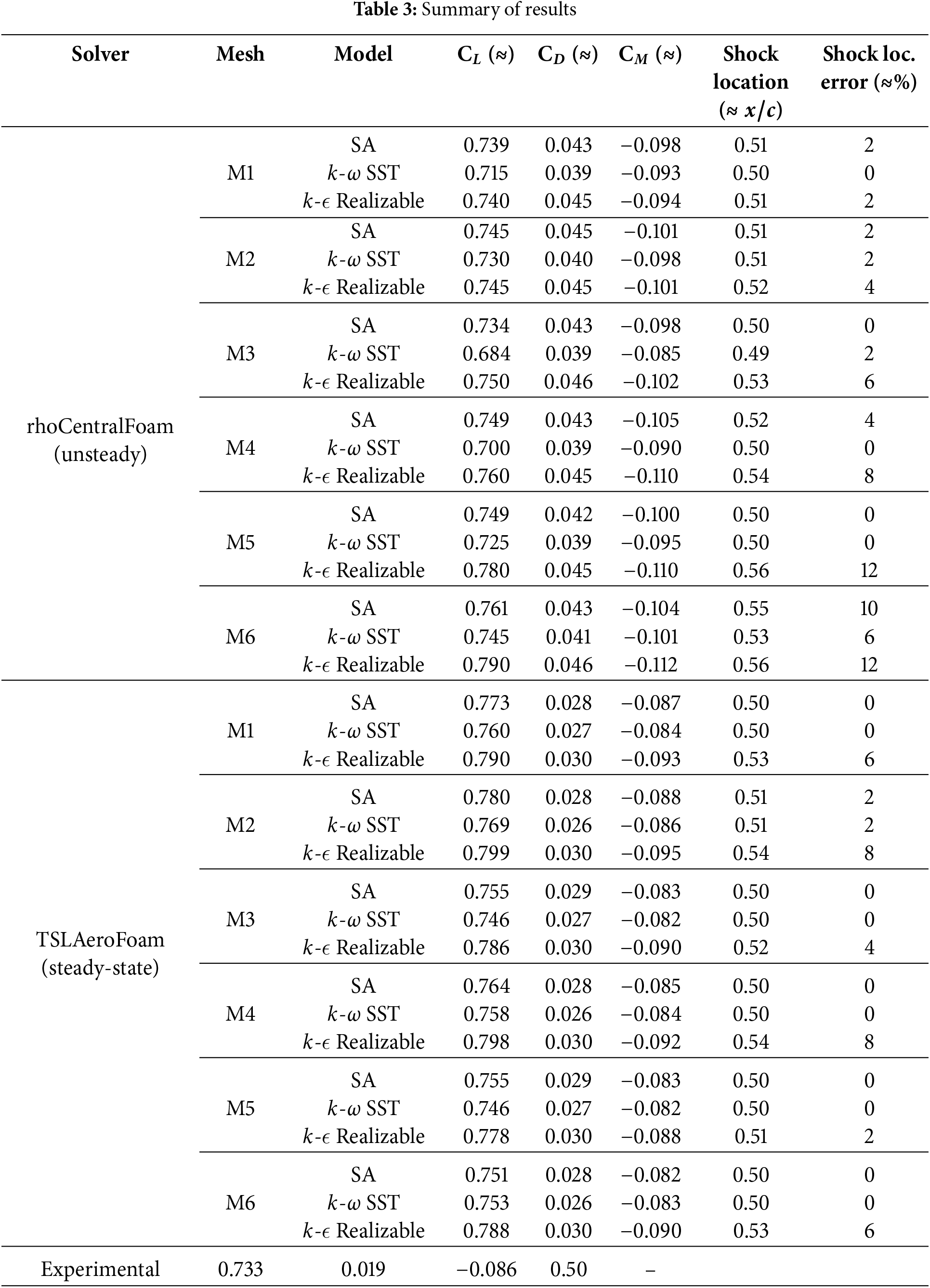
Table 3 summarizes the comprehensive results obtained in this study. The lift coefficient predictions from rhoCentralFoam generally show excellent agreement with the experimental value of CL=0.733, with deviations mostly within 2%. In contrast, TSLAeroFoam tends to slightly overpredict CL by around 4% on average, but provides better drag estimates. The CD predictions show larger discrepancies compared to the experiment. On the experimental side, these discrepancies may be linked to wind tunnel wall interference effects and the high sensitivity of drag to small variations in angle of attack; at transonic speeds, even minor angular deviations can produce large differences in drag. From the numerical perspective, possible differences related to transition modeling—since the simulations assume fully turbulent flow while the experiments may involve transitional effects—and inherent limitations of RANS turbulence models in predicting shock-induced separation and viscous losses may also contribute to systematic overprediction. Regarding shock position, the k-ω SST model performs best, keeping the errors typically below 2% across both solvers. SA also provides reasonable predictions, while the k-ϵ Realizable model exhibits the largest deviations, displacing shocks downstream by up to 12% in some configurations. It can be also seen that turbulence model choice has the strongest influence on predictive accuracy. TSLAeroFoam demonstrated generally better performance in predicting drag and moment coefficients, with the k-ω SST and SA models again proven to be more reliable than the k-ϵ Realizable model. Overall, rhoCentralFoam provides superior CL predictions at the cost of higher computational expense, while TSLAeroFoam achieves efficient convergence and reasonable shock predictions, making it suitable for routine analysis when fine near-wall resolution is used. It should be noted that the simulations are based on the ideal gas and fully turbulent flow assumptions, which may influence the results.

4  Conclusions

This study systematically evaluated the interdependent effects of near-wall resolution, mesh density, and turbulence model choice on transonic shock-boundary layer interaction predictions for the RAE2822 airfoil. The main findings are:

•   The rhoCentralFoam solver achieved generally better lift predictions, staying within about 2% of the experimental value, while TSLAeroFoam tended to overpredict by around 4%.

•   The k-ω SST model provided the most reliable shock predictions, with errors typically below 2% across both solvers. Spalart-Allmaras also performed reasonably well, while the k-ϵ Realizable model showed the largest deviations.

•   Turbulence model choice plays the dominant role in predictive accuracy in transonic CFD simulations, and with appropriate near-wall resolution the influence of global mesh density remains secondary.

•   The TSLAeroFoam solver showed generally better performance in terms of drag and moment coefficient predictions.

•   The rhoCentralFoam solver captured unsteady lift-generating flow physics more accurately but required substantially higher computational cost. TSLAeroFoam achieved efficient convergence and provided reasonable predictions.

For maximum fidelity, unsteady rhoCentralFoam with k-ω SST at y+≈1 is recommended. When computational resources are limited, steady simulations using the k-ω SST or Spalart-Allmaras models provide a practical balance between accuracy and efficiency in transonic flow predictions. It should be noted that this study was limited to the fully turbulent flow assumption for a single airfoil geometry, and more advanced modeling approaches were not explored, which can be addressed in future studies.

Acknowledgement: Not applicable.

Funding Statement: The author received no specific funding for this study.

Availability of Data and Materials: The author confirms that the data supporting the findings of this study are available within the article.

Ethics Approval: Not applicable.

Conflicts of Interest: The author declares no conflicts of interest to report regarding the present study.

References

1. Guo H, Zhang C, Lv B, Yu L. Numerical simulation research on static aeroelastic effect of the transonic aileron of a high aspect ratio aircraft. Comput Model En Sci. 2022;132(3):991–1010. doi:10.32604/cmes.2022.020638. [Google Scholar] [CrossRef]

2. Al-Rbaihat R, Saleh K, Malpress R, Buttsworth D. Experimental investigation of a novel variable geometry radial ejector. Appl Therm Eng. 2023;233(2):121143. doi:10.1016/j.applthermaleng.2023.121143. [Google Scholar] [CrossRef]

3. Widiawaty CD, Siswantara AI, Budiyanto MA, Andira MA, Adanta D, Syafei MHG, et al. Analysis of mesh resolution effect to numerical result of CFD-ROM: turbulent flow in stationary parallel plate. CFD Lett. 2024;16(8):1–17. doi:10.37934/cfdl.16.8.117. [Google Scholar] [CrossRef]

4. Kulkarni S, Chapman C, Shah H. Computational fluid dynamics (CFD) mesh independency study of a straight blade horizontal axis tidal turbine. Preprints. 2016:2016080008. doi:10.20944/preprints201608.0008.v1. [Google Scholar] [CrossRef]

5. Hashimoto A, Ishida T, Ohmichi Y, Aoyama T, Yamamoto T, Hayashi K. Current progress in unsteady transonic buffet simulation with unstructured grid CFD code. In: AIAA Aerospace Sciences Meeting; 2018 Jan 8–12; Kissimmee, FL, USA. doi:10.2514/6.2018-0788. [Google Scholar] [CrossRef]

6. Duggirala R, Roy CJ, Schetz JA. Analysis of interference drag for strut-strut interaction in transonic flow. AIAA J. 2011;49(3):449–62. doi:10.2514/1.45703. [Google Scholar] [CrossRef]

7. Xie A, Yan W, Zhou J. Investigation of shockwave-turbulent boundary layer interaction in transonic compressor rotor37. In: First Aerospace Frontiers Conference (AFC 2024); 2024 Apr 12–15; Xi’an, China. p. 568–74. [Google Scholar]

8. Yi W, Ji L, Tian Y, Shao W, Li W, Xiao Y. An aerodynamic design and numerical investigation of transonic centrifugal compressor stage. J Therm Sci. 2011;20(3):211–7. doi:10.1007/s11630-011-0460-y. [Google Scholar] [CrossRef]

9. Soda A. Numerical investigation of unsteady transonic shock/boundary-layer interaction for aeronautical applications. Tech Rep. DLR Deutsches Zentrum für Luft- und Raumfahrt e.V.; 2007 [Google Scholar]

10. Petrocchi A, Barakos G. Transonic buffet simulation using a partially-averaged navier-stokes approach. Aerosp Sci Technol. 2024;149(5):109134. doi:10.1016/j.ast.2024.109134. [Google Scholar] [CrossRef]

11. Johnston LJ. Computational fluid dynamics analysis of multi-element, high-lift aerofoil sections at transonic manoeuvre conditions. Proc Institut Mech EngbPart G J Aerosp Eng. 2011;226(8):912–29. doi:10.1177/0954410011417541. [Google Scholar] [CrossRef]

12. Galpin P, Hansen T, Scheuerer G, Kelly R, Hickman A, Jemcov A, et al. Validation of transonic axial compressor stage unsteady-state rotor-stator simulations. In: Proceedings of the ASME Turbo Expo 2017: Turbomachinery Technical Conference and Exposition; 2017 Jun 26–30; Charlotte, NC, USA. doi:10.1115/GT2017-64786. [Google Scholar] [CrossRef]

13. Hosangadi A, Ahuja V, Lee YT. Simulations of transonic diffuser-volute system using hybrid unstructured CFD. In: ASME International Mechanical Engineering Congress and Exposition; 2000 Nov 5–10; Orlando, FL, USA. p. 55–62. doi:10.1115/IMECE2000-1671. [Google Scholar] [CrossRef]

14. Coratger T, Farag G, Zhao S, Boivin P, Sagaut P. Large-eddy lattice-boltzmann modeling of transonic flows. Phys Fluids. 2021;33(11):115112. doi:10.1063/5.0064944. [Google Scholar] [CrossRef]

15. Zhou H, Xie F, Ji T, Zhang X, Zheng C, Zheng Y. Fast transonic flow prediction enables efficient aerodynamic design. Phys Fluids. 2023;35(2):026109. doi:10.1063/5.0138946. [Google Scholar] [CrossRef]

16. Jia X, Gong C, Ji W, Li C. An accuracy-enhanced transonic flow prediction method fusing deep learning and a reduced-order model. Phys Fluids. 2024;36(5):56101. doi:10.1063/5.0204152. [Google Scholar] [CrossRef]

17. Mufti B, Bhaduri A, Ghosh S, Wang L, Mavris DN. Shock wave prediction in transonic flow fields using domain-informed probabilistic deep learning. Phys Fluids. 2024;36(1):016121. doi:10.1063/5.0185370. [Google Scholar] [CrossRef]

18. Al-Rbaihat R, Saleh K, Malpress R, Buttsworth D, Alahmer H, Alahmer A. Performance evaluation of supersonic flow for variable geometry radial ejector through CFD models based on DES-turbulence models, GPR machine learning, and MPA optimization. Int J Thermofluids. 2023;20:100487. doi:10.1016/j.ijft.2023.100487. [Google Scholar] [CrossRef]

19. Cook PH, Firmin MCP, McDonald MA. Aerofoil RAE 2822: pressure distributions, and boundary layer and wake measurements. RAE; 1977. [Google Scholar]

20. Jinks E, Bruce P, Santer M. Optimisation of adaptive shock control bumps with structural constraints. Aerosp Sci Technol. 2018;77(1):332–43. doi:10.1016/j.ast.2018.03.010. [Google Scholar] [CrossRef]

21. Modesti D, Pirozzoli S. A low-dissipative solver for turbulent compressible flows on unstructured meshes, with OpenFOAM implementation. Comput Fluids. 2017;152(1):14–23. doi:10.1016/j.compfluid.2017.03.026. [Google Scholar] [CrossRef]

22. Rahman MM, Zhang X, Hasan K, Chen S. RANS flow computation around transonic RAE2822 airfoil with a new SST turbulence model. MIST Int J Sci Technol. 2024;12:23–8. doi:10.47981/j.mijst.12(02)2024.477(23-27). [Google Scholar] [CrossRef]

23. Yun TIA, Gao S, Liu P, Wang J. Transonic buffet control research with two types of shock control bump based on RAE2822 airfoil. Chin J Aeronaut. 2017;30(5):1681–96. doi:10.1016/j.cja.2017.08.009. [Google Scholar] [CrossRef]

24. NASA. RAE2822 transonic airfoil validation data. [cited 2025 Jan 22]. Available from: https://www.grc.nasa.gov/www/wind/valid/raetaf/raetaf.html. [Google Scholar]

25. Greenshields CJ, Weller HG, Gasparini L, Reese JM. Implementation of semi-discrete, non-staggered central schemes in a colocated, polyhedral, finite volume framework, for high-speed viscous flows. Int J Numer Methods Fluids. 2010;63(1):1–21. doi:10.1002/fld.2069. [Google Scholar] [CrossRef]

26. Kurganov A, Tadmor E. New high-resolution central schemes for nonlinear conservation laws and convection-diffusion equations. J Comput Phys. 2000;160(1):241–82. doi:10.1006/jcph.2000.6459. [Google Scholar] [CrossRef]

27. Kumar M, Sahoo R, Behera S. Design and numerical investigation to visualize the fluid flow and thermal characteristics of non-axisymmetric convergent nozzle. Eng Sci Technol Int J. 2019;22(1):294–312. doi:10.1016/j.jestch.2018.10.006. [Google Scholar] [CrossRef]

28. Kaya MN, Satcunanathan S, Meinke M, Schröder W. Leading-edge noise mitigation on a rod-airfoil configuration using regular and irregular leading-edge serrations. Appl Sci. 2025;15(14):7822. doi:10.3390/app15147822. [Google Scholar] [CrossRef]

29. Canteros ML, Polanský J. Review and comparison of two OpenFOAM solvers: rhocentralfoam and sonicfoam. EPJ Web Conf. 2024;299:1005. doi:10.1051/epjconf/202429901005. [Google Scholar] [CrossRef]

30. Kim J, Kim K. A development and verification of density based solver using LU-SGS algorithm in OpenFOAM. In: ICAS 2014, 29th Congress of the International Council of the Aeronautical Sciences; 2014 Sep 7–12; St. Petersburg, Russia. p. 375. [Google Scholar]

31. You KK, Ha JH, Lee SC. An automated aerodynamic analysis system in missile based on open-source software. Int J Aeronaut Space Sci. 2023;24(3):592–605. doi:10.1007/s42405-022-00558-0. [Google Scholar] [CrossRef]

32. Spalart P, Allmaras S. A one-equation turbulence model for aerodynamic flows. In: 30th Aerospace Sciences Meeting and Exhibit; 1992 Jan 6–9; Seattle, WA, USA. p. 439. [Google Scholar]

33. Menter FR. Two-equation eddy-viscosity turbulence models for engineering applications. AIAA J. 1994;32(8):1598–1605. doi:10.2514/3.12149. [Google Scholar] [CrossRef]

34. Noorollahi Y, Ziabakhsh Ganji MJ, Rezaei M, Tahani M. Analysis of turbulent flow on tidal stream turbine by RANS and BEM. Comput Model Eng Sci. 2021;127(2):515–32. [Google Scholar]

35. Shih TH, Liou WW, Shabbir A, Yang Z, Zhu J. A new k-ϵ eddy viscosity model for high Reynolds number turbulent flows. Comput Fluids. 1995;24(3):227–38. [Google Scholar]

36. Fuhrman DR, Li Y. Instability of the realizable k-ϵ turbulence model beneath surface waves. Phys Fluids. 2020;32(11):115108. doi:10.1063/5.0029206. [Google Scholar] [CrossRef]