Channel-Attention DenseNet with Dilated Convolutions for MRI Brain Tumor Classification

1  Introduction

Brain tumors are a diverse group of intracranial growths, ranging from benign to highly malignant, each varying in growth rate and prognosis. According to the World Health Organization (WHO), brain tumors are labeled into more than a hundred and twenty types, making diagnosis and treatment complex [1]. These tumors can be primary, arising in the brain, or secondary, metastasizing from other body parts [2]. The diagnosis of a brain tumor presents significant complications. Early symptoms such as headache, nausea, and psychosis are often non-specific and can be mistaken for less severe health conditions [3]. Furthermore, the critical location of the tumor can complicate the choice of surgery, emphasizing the importance of accurate diagnostic tools. Magnetic resonance imaging (MRI) is the gold standard for diagnosing brain tumors because it can differentiate between soft tissues and accurately localize the tumor [4]. However, MRI requires interpretation by highly skilled radiologists and can be time-consuming, potentially delaying treatment decisions. In addition, the subtle presentation of some tumors may lead to discrepancies between interpretation and subsequent treatment [5]. Advances in imaging techniques and computational tools have opened new possibilities for increasing analysis accuracy. The integration of artificial intelligence (AI) into imaging has shown the potential to improve the detection and characterization of brain tumors, providing tools that assist radiologists by highlighting areas of potential concern and reducing the possibility of human compliance [6]. Developing such AI-based diagnostic tools requires complex datasets and new algorithms that can detect complex patterns in imaging data. These tools aim to increase accuracy and reduce the time between the onset of symptoms and the start of treatment, which is essential for patient outcomes [7]. While MRI remains an important diagnostic tool for brain tumors, the addition of AI promises to solve existing challenges by improving the speed and potential accuracy of diagnosis. This integration signals a shift towards a more reliable and effective diagnostic approach, ultimately aimed at enhancing prognostic outcomes for patients with brain tumors. MRI is an essential tool in the diagnosis and management of brain tumors. It provides detailed anatomical imaging of the brain, allowing for accurate tumor identification and characterization [8]. MRIs use magnetic fields and radio waves to create contrast images between tissues, including tumors and normal brain tissue. This capability is valuable in neurology, where such accuracy is critical for effective treatment management. One of the main advantages of MRI over other imaging modalities, such as computed tomography (CT) scans, is its contrast enhancement, which is important in determining the boundaries and extent of brain tumors [9]. MRI can also differentiate between edema (swelling), tumor infiltration, and normal tissue, which helps assess the tumor’s aggressiveness and potential response to therapy [10]. MRI helps in the initial diagnosis and is crucial in the follow-up and monitoring of brain tumors. It is used to assess tumor growth, evaluate the effectiveness of treatments, and monitor for recurrence post-treatment [11]. Various specialized MRI techniques enhance its diagnostic power. Functional MRI (fMRI) helps identify the specific function of the parts of the brain affected by tumors, which is important for surgical planning to avoid areas that perform vital functions such as speech, movement, and cognition [12]. Magnetic Resonance Spectroscopy (MRS) gives biochemical records of brain tissues, which could differentiate tumor types and perceive tumor metabolism traits [13]. Diffusion tensor imaging (DTI) provides insight into how the integrity of white matter tissue may be affected by tumor growth to help map the surgical approach and assess the impact of tumors on brain connectivity [14].

Despite its advantages, MRI does have limitations. This time-consuming and expensive procedure can be uncomfortable for patients, especially those who are afraid to lie down or remain still during the scanning process. Furthermore, the interpretation of MRI results depends on the radiologist’s expertise, which can vary and affect diagnostic accuracy [15]. MRI remains the cornerstone of brain tumor diagnosis, treatment planning, and management. Its ongoing development with advances in AI and machine learning promises to be more accurate and efficient in the future, potentially changing the landscape of brain tumor diagnosis and care [16]. Deep learning, a subset of machine learning characterized by networks that can learn unsupervised from unstructured or anonymized data, has transformed the medical picture over the past decade. Its flexibility enables it to perform complex visualization tasks with high accuracy and speed, often exceeding traditional image processing.

Early applications of deep learning in medical imaging included the use of convolutional neural networks (CNNs), which automatically learn spatial patterns of objects through backpropagation, a significant departure from the previous practice where various components had to be fine-tuned manually [17]. CNNs have been widely adopted for various tasks in medical imaging, including classification, detection, and segmentation of medical images. One of the first successes was the use of AlexNet [18], which significantly outperformed all previous competitors in the ImageNet competition. This success has spurred further research and development in deep learning frameworks, resulting in groundbreaking models such as GoogleNet and VGGNet, improving the network’s depth and complexity [19]. The introduction of ResNet in 2015 marked another milestone in deep learning, making it feasible to train models with hundreds or even thousands of layers successfully. ResNet employs skip connections, or shortcuts, to skip over certain layers. Typical CNNs had a problem with vanishing gradients as they grew deeper. In order to understand the behavior of ResNet, a similarity between two well-known CNNs, Inception and ResNet, were discussed in [20].

Recently, the original focus and object transformation methods for natural language processing tasks have been adapted for clinical imaging. These models, such as Vision Transformer (ViT), are starting to show promising results, as they handle the inter-pixel dependencies in an image differently than CNN [21]. The DenseNet architecture is used to improve its performance in MRI-based brain tumor segmentation. These modifications include the integration of dilated convolutions, which expand the receptive field without increasing computational cost, and an attention mechanism that directs the model’s focus to key areas within the MRI images. Together, these enhancements allow for more precise feature extraction and segmentation, addressing the complexities of brain tumor identification in MRI scans and improving diagnostic accuracy and reliability.

The application of deep learning in medical imaging is not limited to structural imaging. Still, it extends to functional imaging modalities such as positron emission tomography (PET), MRI, etc., which are only visible to the naked eye [22]. Additionally, deep learning has facilitated the development of predictive models, leveraging historical data to forecast outcomes such as disease progression and treatment responses [23]. With ongoing advancements in computing power, the availability of large, labeled datasets, and sophisticated neural network architectures, the application of deep learning in medical imaging continues to expand rapidly. This study focuses on addressing the technical limitations of existing deep learning approaches in brain tumor diagnosis by introducing significant advancements to the DenseNet architecture:

•   Herein, we propose an advanced brain tumor detection model. Our proposed model incorporates dilated convolutions to expand the receptive field without increasing the computational cost, enabling the model to capture fine-grained spatial details crucial for accurate segmentation of complex tumor structures in MRI images. The focus on relevant regions of the MRI scans improves the model’s ability to differentiate between tumor and non-tumor areas, thereby increasing diagnostic accuracy.

•   The effectiveness of proposed models is accompanied by discussions on their adaptability to clinical practice, addressing potential challenges like interpretability and user-friendly interfaces to promote their widespread application.

•   By emphasizing technical contributions, particularly the integration of dilated convolutions and attention mechanisms, this study highlights the modified DenseNet’s capability to overcome existing challenges in MRI-based brain tumor detection, paving the way for reliable and efficient clinical diagnostics. This research is significant in the advancement of AI in medical imaging. Specifically, it helps improve the role of MRI technologies in the diagnosis and treatment planning of brain tumors.

The rest of the paper is organized as follows: Section 2 analyzes the related literature and offers a background for the current study. Section 3 describes the methodology, focusing on data collection, development of the DenseNet model with modifications, and evaluation metrics. Section 4 is the results section that compares and analyzes performance metrics of the modified DenseNet and traditional models. Section 5 summarizes the conclusions drawn from the study, the constraints encountered, and the possible solutions. The paper concludes with Section 5, which contains a concluding section and recommendations for future research. Furthermore, each component includes relevant tables and figures to visualize and support the discussion.

2  Related Work

In this section, we present the development of diagnostic techniques from conventional imaging modalities to advanced AI-powered methods. It emphasizes critical studies showing the success of deep learning architectures such as CNNs, ResNet, and the original DenseNet models in medical settings. This will be a stepping stone to introducing the modified version of DenseNet. The review places the current research in the framework of the overall scientific discourse and unearths the existing gaps in technologies, which the modified DenseNet aims to fill, thereby rationalizing the need for this research’s innovative method. Conventional approaches to the diagnosis of brain tumors are primarily based on clinical examination and imaging techniques that provide essential insights into the anatomy and function of brain tumors [24]. Traditionally, CT images play a role, especially in early brain scans, due to their ability to rapidly generate images. Acute conditions are adequate for identification but provide limited soft tissue contrast, which is important for detailed brain tumor evaluation [25]. MRI is the preferred imaging tool for brain tumors to differentiate brain tissue types and tumor size, location, and proximity. Advanced MRI techniques with T1- and T2-weighted imaging are also appreciated for their superior ability to obtain a comprehensive image of structures and the possibility of interference to improve the accuracy of the diagnostic appearance by providing a clear distinction between tumor material and surrounding edema [26]. The test has been performed. Despite being informative, biopsies are invasive and carry risks such as possible infection and bleeding. The tumor’s accessibility also limits its applicability [27]. Angiography, involving the injection of a contrast agent to visualize the vascular structure of the brain, has helped plan surgeries for tumors impacting blood vessels or those highly vascular. Coronary heart disease prediction is proposed in [28] using Gaussian Fuzzy C-Means Clustering (GKFCM) with Recurrent Neural Network (RNN). It is evident from the literature that, nuclear medicine techniques like PET and single-photon emission computed tomography (SPECT) are occasionally utilized to assess the metabolic activity of brain tumors. However, due to their high costs and limited availability, they are not routinely used for initial diagnostic purposes [29]. The need for higher diagnostic precision enhanced patient safety, and a better pre-operative understanding of tumors has driven the transition from these conventional methods to more advanced diagnostic approaches. Some initial deep-learning solutions in medical imaging are groundbreaking. They abandoned the more conventional practices of image processing and machine learning in which feature extraction was mainly manual and time-consuming. The arrival of deep learning provided a sound basis for learning features to cut short the need for employing domain expertise, significantly boosting the reliability and speed of medical image analysis, including detecting brain tumors. As one of the first and most impactful medical imaging solutions, deep learning has incorporated CNNs into its suite of tools. CNNs make feature representations by learning from raw data directly and thus do not require feature extraction. AlexNet by [18] started the journey with a deep CNN, which was immediately identified as a viable solution for medical imaging problems. In brain tumor diagnosis, CNNs were initially applied to recognize and demarcate MRI images, such as discontinuing tumor parts with greater precision compared to conventional approaches. One of the first strategies for utilizing deep learning in the medical imagery space was the methodology of transfer learning. Original deep models learned from natural image databases, including the ImageNet databases, were retrained and fine-tuned to distinguish between medical images and identify features such as brain MRIs [30]. Autoencoders, another veteran in deep learning, were applied to unsupervised learning, which involves dimensionality reduction and feature learning from medical images. For brain tumor detection, autoencoders can be applied to pre-train segments of a network for one or more attention tasks, which, in effect, tend to learn a lower-dimensional representation of standard structure in which disruptions signifying tumors are detectable [31]. Early deep learning systems had issues, although they showed promising results. Furthermore, the “black box” nature of early deep models often made it difficult for medical professionals to trust their outputs, as the reasoning behind decisions was not always clear [32]. Integrating deep learning into clinical practice required technical advancements and a better understanding among clinicians of how these tools could be used without replacing the diagnostician. Early successes in deep learning paved the way for broader acceptance and trust in these technologies, underscoring the need for collaborative approaches that combine the best human expertise with automated efficiency. Despite the substantial progress and widespread adoption of AI models in medical imaging, several limitations persist that affect their effectiveness and integration into clinical workflows. These limitations revolve around data dependency, algorithmic transparency, model generalizability, and ethical concerns, each presenting unique challenges to healthcare providers and researchers. AI models, which are intensive learning systems, require large amounts of data for training to achieve high accuracy and reliability. However, such extensive, well-annotated medical imaging datasets are often limited due to privacy concerns, the rarity of certain conditions, and the vast time and expertise required for accurate annotation [33]. Furthermore, suppose the training data does not represent the global population. In that case, the model may exhibit biases, performing well on the demographic it was trained on but poorly on others, leading to unequal healthcare outcomes [34]. Many advanced AI models, particularly those based on deep neural networks, suffer from a lack of transparency, often referred to as the “black box” problem [35]. This opacity makes it difficult for clinicians to understand how decisions are made, a significant barrier to trust and reliance on AI systems for critical diagnostic tasks. The need for explainable AI is crucial in medical settings, where understanding the rationale behind a diagnostic conclusion or treatment recommendation is essential for acceptance and ethical practice [36]. AI models often perform exceptionally well in controlled test environments or specific datasets on which they were trained, but fail to generalize across different populations or medical settings. This issue stems from overfitting, where a model learns the noise and details in the training data to the extent that it negatively impacts the performance of new data [37]. Integrating AI into healthcare raises several ethical concerns, including patient privacy, consent to use medical data for training models, and the potential for increased automation to reduce the role of human clinicians, which could lead to job displacement. Additionally, regulatory bodies are still adapting to the rapid development of AI technologies, and there is a lack of clear guidelines and standards for validating the safety and efficacy of AI-based diagnostic tools [38]. Integrating AI systems into existing clinical workflows poses another set of challenges [39]. These studies highlight the potential of deep learning models in enhancing diagnostic accuracy and set a benchmark for evaluating our modified DenseNet architecture. Despite these advances, prior studies still exhibit important limitations. For example, several CNN-based and Internet of Medical Things (IoMT)-enabled systems for cancer detection demonstrate high accuracy but provide limited interpretability, making it difficult to justify predictions in clinical workflows [40,41]. Other recent brain tumor detection approaches, including step-constant tapered slot antenna (STSA) based early-stage detection [42] and reinforcement learning–driven neural architecture search frameworks [43], show promise but often face challenges in modeling the heterogeneous and irregular morphology of tumor regions. Moreover, many of these models rely on complex or computationally intensive architectures, raising concerns about scalability and generalization to unseen datasets. These gaps highlight the need for an efficient yet interpretable model that can capture multi-scale tumor structures while remaining computationally practical, a motivation that directly underpins the design of our proposed DenseNet variant.

3  Propose Methodology

A Dense Convolutional Network (DenseNet) is a state-of-the-art design that alleviates several inherent problems of conventional convolutional networks, especially those related to the flow and utilization of features. The main idea of DenseNet is connectivity. At the same time, in a CNN, each layer is connected only to a prior layer; in DenseNet, every layer is connected to all prior layers [44]. This characteristic is achieved through feature concatenation rather than summation, resulting in a thinner and more efficient network than a standard CNN. The process presented in Fig. 1 outlines a structured, multistep approach to data preprocessing, ensuring precise and clinically relevant results. Thus, this complex approach allows dramatic changes in learning and performance and corresponds to the high level necessary for medical image analysis and tumor detection.

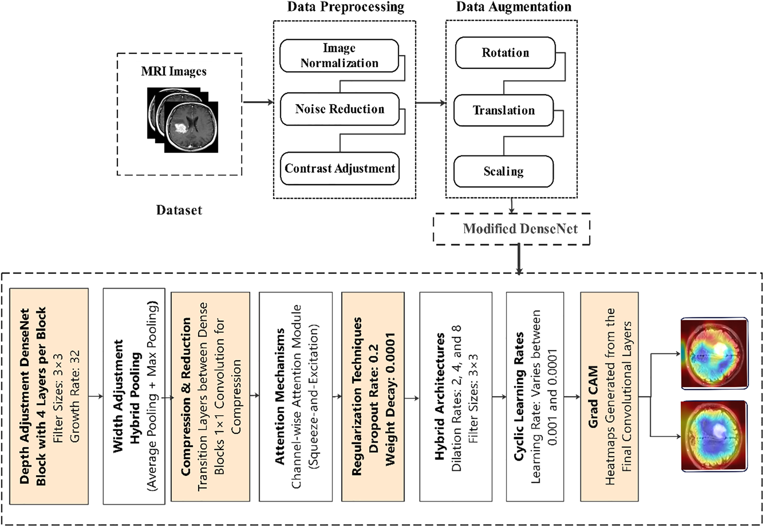
Figure 1: Proposed model

Fig. 1 shows the workflow to detect brain tumors using MRI. Herein, the Data preprocessing begins with normalizing raw data, then noise reduction and contrast enhancement of data images and data augmentation, including data rotation, translation, and scaling. The modified DenseNet incorporates DenseNet blocks with 3 × 3 filters and a growth rate of 32+, hybrid pooling layers, 1 × 1 compression layers, and attention mechanism squeeze-and-excitation dense blocks, as well as dilated convolution with rates of 2, 4 & 8 for more expansive reception fields. The models are regularized using dropout with a rate of 0.2 and weight decay of 0.0001. Applying cyclic learning rates ranging from 0.001 to 0.0001 enhances training effectiveness. Grad-CAM visualization points out the tumor areas, making it possible to interpret and better tumor detection.

3.1 Dataset

BraTS 2020 [45] is rigorously selected and annotated to facilitate the training and testing of machine-learning methods for brain tumor segmentation. The dataset in Table 1 includes multi-parametric MRI scans, which are vital for modeling to reflect the complexity of the brain tumors.

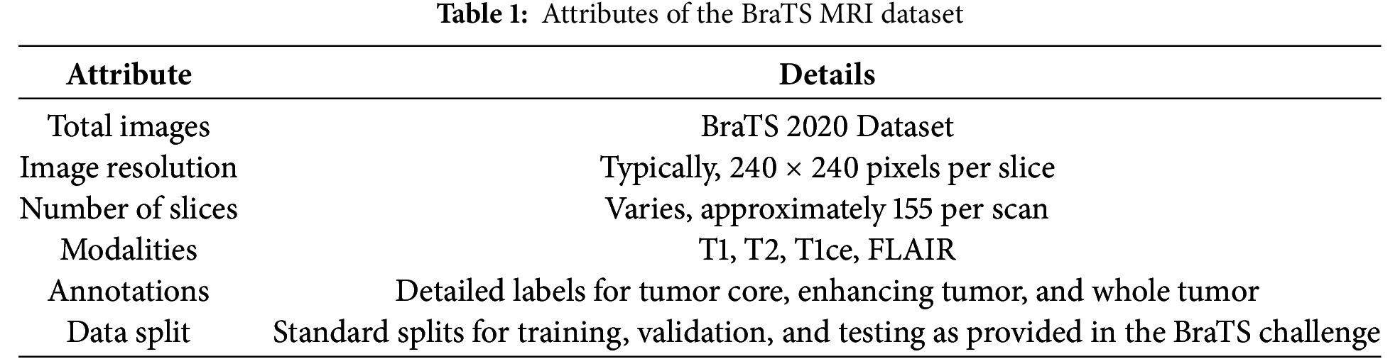
With the BraTS dataset, there is a solid starting point from which a better AI-based model for detecting brain tumors can be developed. The discriminative and comprehensive multi-modal MRI scans of the dataset help the DenseNet architecture solve the problem of brain tumor diagnosis with higher accuracy due to detailed and less abstract learning of peculiarities.

3.2 Preprocessing

Preprocessing is essential for making MRI images as close as possible to the neural network training input data and making it every day. MRI images were then normalized to minimize pixel differences. In particular, image pixel intensity values were normalized such that their mean value was equal to zero and the standard deviation was equal to one. Such normalization helps bring all the input images into the same scale, which is essential, especially since we’re using a neural network. The quantitative conversion is made uniform by applying the same scaling factor, thus increasing the train rates while improving the predictions’ accuracy. Each MRI image is initially normalized by subtracting the mean value and dividing it by the standard deviation. This will also enhance the model’s learning speed and convergence, as it is built on a single standard scale. For each image, the overall mean of pixel intensity is computed. This is the average of the absolute value of its pixels divided by the total number of pixels in the image.

The standard deviation, which measures the spread of pixel intensity values around the mean, is also computed. The formulas for the mean (μ) and standard deviation (σ) are:

μ=1N∑i=1Nxi(1)

σ=1N∑i=1N(xi−μ)2(2)

where xi represents the intensity value of the ith pixel and N is the total number of pixels in the image.

Each pixel intensity xi is transformed using the calculated mean (μ) and standard deviation (σ) to get a new value xi′ such that the resulting image has a mean of zero and a standard deviation of one. Normalization calculated by:

xi′=(xi−μ)σ(3)

MRI images often contain noise from machine vibrations, thermal fluctuations, or operator variability. Gaussian blurring was applied to reduce noise, a technique that uses a Gaussian function to smooth the image, minimizing minor distortions that could obscure important features like tumor regions. This step helps clarify the MRI scans, allowing the model to focus on relevant image details. One effective method for noise reduction in these images is Gaussian blurring, which uses a Gaussian function to smooth the image and reduce the noise level. The Gaussian filter is defined by the Gaussian function, which in two dimensions has the form:

G(x,y)=12πσ2e−x2+y22σ2(4)

here, x and y are the distances from the origin in the horizontal and vertical axes, respectively, and σ is the standard deviation of the Gaussian distribution. The parameter σ controls the extent of smoothing: a larger σ results in more blurring as the function’s width increases.

The image is convolved with the Gaussian kernel to produce the smoothed image. The convolution of an image I with the Gaussian kernel G is given by:

I′(x,y)=(G∗I)(x,y)=∑i=−kk∑j=−kkG(i,j)⋅I(x−i,y−j)(5)

where ∗ denotes convolution, I′(x,y) is the pixel value of the processed image at the position (x,y), and k is the kernel size, typically chosen based on σ (e.g., k=3σ).

3.3 Data Augmentation

Data augmentation techniques are extensively used to increase the diversity of the training data and simulate various real-world scenarios. Augmentation helps combat overfitting and enhances the model’s generalization ability to new, unseen data. Here are the key augmentation strategies employed. Several data augmentation techniques are used to simulate a range of clinical imaging scenarios. Random rotations within a range of −10 to 10 degrees address variations in patient positioning during MRI scans. Translations along the horizontal and vertical axes simulate slight shifts in perspective while scaling adjustments mimic different resolutions encountered in clinical practice. Additionally, the snapshots are scaled by other factors to reflect the diversity in image resolutions encountered in one-of-a-kind clinical settings. Additionally, we carry out horizontal and vertical flips on the snapshots, growing the dataset’s variability and ensuring the version can efficaciously cope with photographs in extraordinary orientations. Lastly, elastic deformation is used, using non-linear ameliorations to the pictures to emulate anatomical variations and the variations that can increase in MRI scan acquisitions. These augmentation strategies decorate our version’s robustness, preparing it to cope with real international imaging variations.

A random angle rotates images θ, where θ is chosen uniformly from a range, e.g., [−10∘,10∘]. The rotation transformation for a point (x,y) in the image can be represented using a rotation matrix:

[x′y′]=[cosθ−sinθsinθcosθ][xy](6)

This transformation rotates the pixel coordinates (x,y) to new coordinates (x′,y′), altering the image’s orientation without changing its dimensions.

Images are translated randomly in both the X and Y axes. If tx and ty represent the translation distances along the X and Y axes, respectively; each pixel (x,y) in the original image is moved to (x+tx,y+ty). This can be expressed as:

[x′y′]=[10tx01ty001][xy1](7)

This matrix operation shifts the location of each pixel, effectively mimicking the shift in imaging perspective.

Scaling is applied to simulate different image resolutions. A scaling factor s uniformly chosen from a predefined range, e.g., [0.9,1.1], resizes the image. The scaling transformation for a point (x,y) is:

[x′y′]=[s00s][xy](8)

This adjusts each pixel’s coordinates to expand or contract the image, reflecting different resolutions encountered in clinical settings. Flipping operations are either horizontal or vertical. For horizontal flipping, each pixel’s x-coordinate is inverted:

x′=image width−x−1(9)

For vertical flipping, the y-coordinate is inverted:

y′=image height−y−1(10)

These transformations flip the image across the respective axes, enhancing the dataset’s variability by accommodating images in different orientations.

Elastic deformation introduces non-linear transformations that mimic natural anatomical variations. It uses a displacement field. (Δx,Δy), where each displacement component is sampled from a Gaussian distribution. The transformed coordinates (x′,y′) are then given by:

x′=x+Δx(x,y),y′=y+Δy(x,y)(11)

A Gaussian kernel typically smooths these fields to ensure realistic deformations and not introduce sharp artifacts.

3.4 Modified DenseNet

The DenseNet used in our study is configured with specific characteristics optimized for segmenting and classifying brain tumors from MRI data.

DenseNet architectures are mainly known for their parameter usage and feature propagation efficiency. The core idea is that each layer is directly connected to every other layer in a feed-forward fashion. Mathematically, for a given layer ll, the feature maps of all preceding layers [x0,x1,…,xl−1] are used as inputs:

xl=Hl([x0,x1,…,xl−1])(12)

where Hl(⋅) represents a composite function of operations—Batch Normalization (BN), followed by a ReLU activation and a 3 × 3 Convolution (Conv).

To better capture the complexities of MRI data, we increase the depth of the network. Deeper networks generally perform better at learning features from complex data. However, to prevent the vanishing gradient problem, each DenseNet block is equipped with skip connections, ensuring that the gradient can propagate back through the network without significant loss:

Each layer in the DenseNet is designed to receive contributions from all preceding layers. The output of the llth layer (xl) is formulated using a function that combines the outputs of all previous layers through skip connections and a transformation Hl. Mathematically, this is represented as:

xl=xl−1+Hl([x0,x1,…,xl−1])(13)

here xl−1 the output from the previous layer, and Hl represents a composite function of batch normalization (BN), ReLU activation, and convolution (Conv).

The function Hl applied to the concatenated outputs of all preceding layers is defined as:

Hl([x0,x1,…,xl−1]=Conv(ReLU(BN(Concat([x0,x1,…,xl−1]))))(14)

xl=xl−1+Conv(ReLU(BN(Concat([x0,x1,…,xl−1]))))(15)

Hl([x0,x1,…,xl−1])=Conv(ReLU(BN(Concat([x0,x1,…,xl−1]))))Hl(16)

For attention mechanism application:

Al=σ(Conv(Hl))(17)

For combining attention with feature maps:

xl=xl−1+Al(Hl([x0,x1,…,xl−1]))(18)

where σ denotes the sigmoid function that scales the output of a convolutional layer applied to the feature maps, enabling selective emphasis on relevant features in the image.

We introduce dilated convolutions in specific layers to increase the receptive field without losing resolution or excessively increasing the number of parameters. Dilated convolutions help in expanding the kernel’s footprint, capturing a more significant context without the downsampling typically used in deeper networks:

Hl=Convdilated(BN(ReLU([x0,x1,…,xl−1])))(19)

where Convdilated represents a convolution operation with a dilation rate greater than 1, expanding the kernel’s reach to capture more spatial context.

Hl=Convdilated(BN(ReLU(Concat([x0,x1,…,xl−1]))))(20)

Convdilated represents the convolution operation equipped with a dilation rate greater than 1. This dilation rate expands the spatial coverage of the convolution kernel, allowing it to encompass a larger area of input features without increasing the number of parameters as much as increasing the kernel size directly would.

The attention mechanism in our model is a channel-wise attention module that enhances the model’s ability to focus on relevant MRI regions associated with tumor characteristics. By dynamically adjusting the weights of feature channels, this mechanism emphasizes critical features while suppressing less relevant information, thereby improving segmentation accuracy and diagnostic precision.

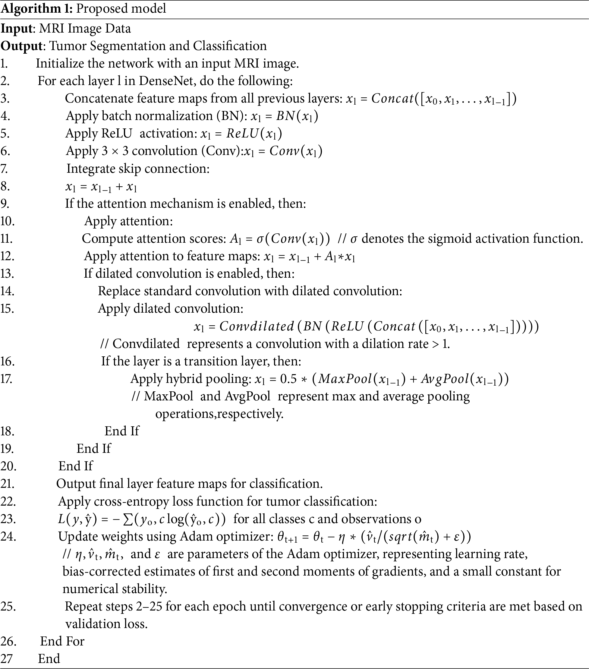
Algorithm 1 demonstrates the implementation of segmenting and classifying brain tumors using a modified DenseNet architecture, which proceeds with MRI images by concatenating features, performing batch normalization, applying ReLU activation, performing convolutions, implementing skip connections, and optionally using attention and dilated convolutions for a more excellent detailed capture, followed by tumor classification optimized by the Adam optimizer.

The dilation rate effectively spaces out the kernel elements, enabling the capture of information from a wider field without a direct sampling of every single intermediate point within the receptive field. Thus, resolution is maintained, and computational load is reduced.

A hybrid pooling strategy is used in transition layers to preserve critical spatial details while reducing dimensionality. This strategy combines average pooling and max pooling, aiming to retain prominent features while lowering the output dimensions smoothly:

Pl=12(MaxPool(xl−1)+AvgPool(xl−1))(21)

The following steps train our DenseNet model, each incorporating key techniques to optimize performance.

The primary loss function used is the cross-entropy loss for classification tasks, defined as:

L(y,y^)=−∑c=1Myo,clog(y^o,c)(22)

yo,c is a binary indicator (0 or 1) if the class label c is the correct classification for observation o. y^o,c is the predicted probability that observation o is of class c. M is the number of classes.

We use the Adam optimizer to update the weights in the network, which computes adaptive learning rates for each parameter. The update rule for Adam is given by:

θt+1=θt−ηv^tm^t+ϵ(23)

θ are the parameters of the model. η is the learning rate. v^t and m^t are the bias-corrected estimates of the first and second moments of the gradients, respectively? ϵ is a small constant added to improve numerical stability.

The DenseNet model is well-suited for the complexities of detecting and segmenting brain tumors from MRI images, leveraging the full potential of its architectural innovations.

3.5 Evaluation Metrics

To evaluate the effectiveness of the DenseNet model in detecting and segmenting brain tumors, we use several key performance metrics that are standard in medical imaging tasks:

Accuracy is the most straightforward and most intuitive performance measure [40]. It is calculated as the ratio of correctly predicted observations to the total observations. Sensitivity measures the proportion of actual positives that are correctly identified as such and is crucial for medical diagnostics, where missing a condition can be critical. Specificity, on the other hand, measures the proportion of actual negatives that are correctly identified. Precision is the ratio of correctly predicted positive observations to the total predicted positives. The F1 Score is the weighted average of Precision and Recall. Therefore, this score takes both false positives and false negatives into account. It is beneficial when the class distribution is uneven. The Area Under the Receiver Operating Characteristic Curve (AUC-ROC) is a graphical plot that illustrates the diagnostic ability of a binary classifier system as its discrimination threshold is varied. The AUC represents the degree or measure of separability.

3.6 Interpretability Techniques

To make the model’s decisions understandable, especially in a clinical setting where understanding the reasoning behind a diagnosis is as important as the diagnosis itself, we employ Gradient-weighted Class Activation Mapping (Grad-CAM) and Layer-wise Relevance Propagation (LRP) techniques:

Grad-CAM uses the gradients of any target concept (like a decision output) flowing into the final convolutional layer to produce a coarse localization map, highlighting essential regions in the image for predicting the concept:

LcGrad−CAM=ReLU(∑αkcAk)(24)

where αkc is the gradient importance weight for the class c, and Ak represents the activation maps.

LRP is used to decompose the output predictions of a network by propagating the prediction backward through the layers to assign a relevance score to each input pixel:

Ri=∑jaiwij∑iaiwijRj(25)

where ai are the activations of a layer i, wij are the weights between layers i and j, and Rj is the relevance of neuron j in the subsequent layer. These metrics and techniques provide a robust framework for evaluating and enhancing our DenseNet model’s performance.

3.7 Setup and Computational Tools

This research tested the modified DenseNet algorithm’s performance in detecting brain tumors from MRI images with a well-scripted algorithm and computational tools. This section describes the hardware and software platforms and libraries and the overall environment utilized for the current analyses.

Applying this specific computational model offered a stable and high-performance environment where experiments can be run to assess the modified DenseNet model. Powerful GPUs enabled rapid model iterations and experiments, while an extensive software ecosystem supported all aspects of the machine learning workflow, from preliminary data processing to model building to the results analysis and visualization.

4  Results and Discussion

This section presents the performance of the modified DenseNet structure in identifying and segmenting brain tumors from the MRI images. It details the metrics, including accuracy, precision, and recall, and it also discusses the improvements over the standard models alongside graphical representations of the model’s efficiency.

4.1 Performance Metrics and Visualization

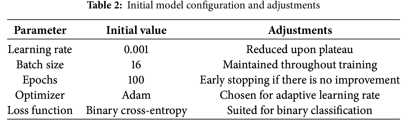
To visualize the training progress and the effects of our adjustments, we summarized them in tables and employed several graphical representations. Initial Model Configuration and Adjustments are outlined in Table 2.

Training adjustment and outcomes are summarized in Table 3.

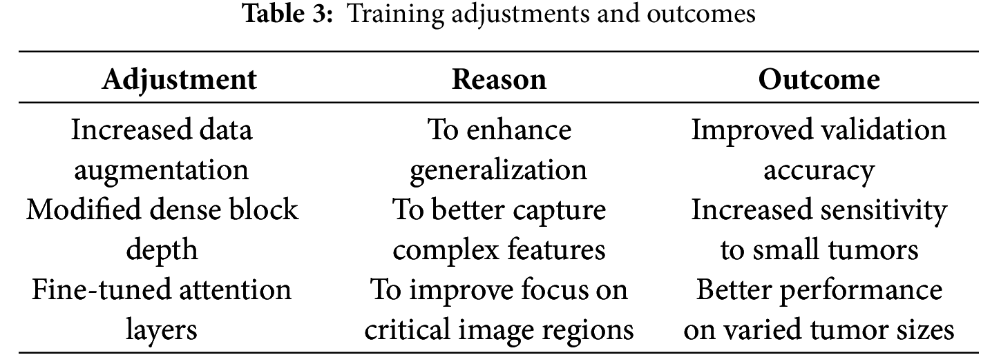
Fig. 2 illustrates the decline in loss values over time, marked at points where adjustments were made, showing their immediate and long-term effects on model performance.

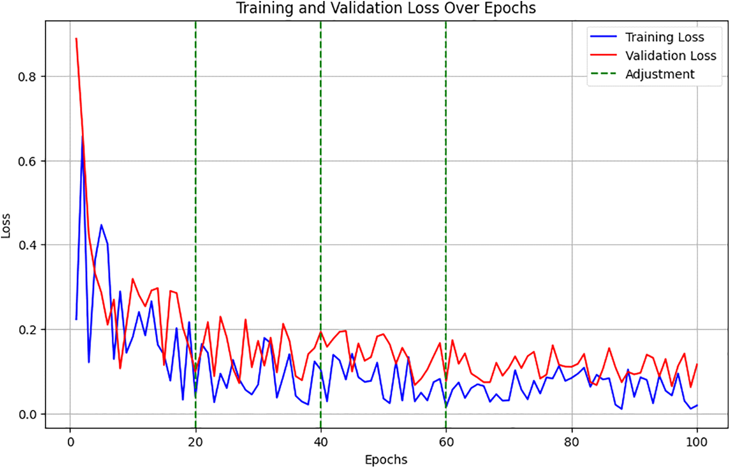
Figure 2: Training and validation loss over epochs

Training and validation loss over epochs showed a decreasing trend, with noted improvements following each adjustment. Fig. 3 charts the trajectory of accuracy improvements, linking these directly to the specific adjustments in data augmentation, dense block configuration, and attention mechanisms. It demonstrated accuracy improvements, correlating these gains with particular changes in model configuration and training strategy.

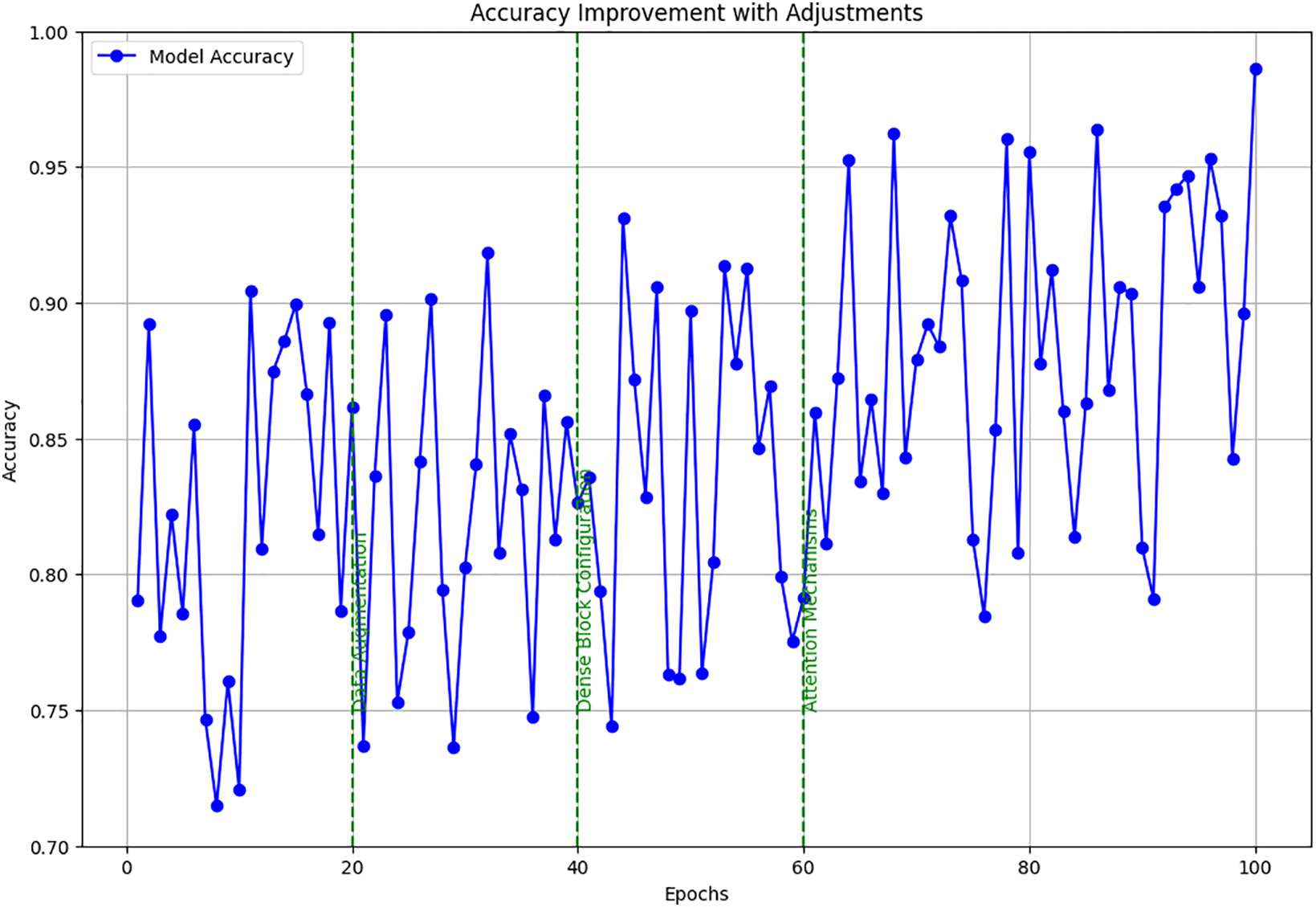
Figure 3: Accuracy improvement with adjustments

The detailed setup and continuous adjustments allowed for fine-tuning the DenseNet model’s capabilities in detecting brain tumors from MRI images. It ensured robustness and accuracy, making it highly effective for clinical applications. These tables and figures provide a clear, structured view of how systematic changes to the training approach directly contributed to performance enhancements.

4.2 Evaluation of Model Performance

The results of the model’s performance across different thresholds and conditions are summarized in Table 4.

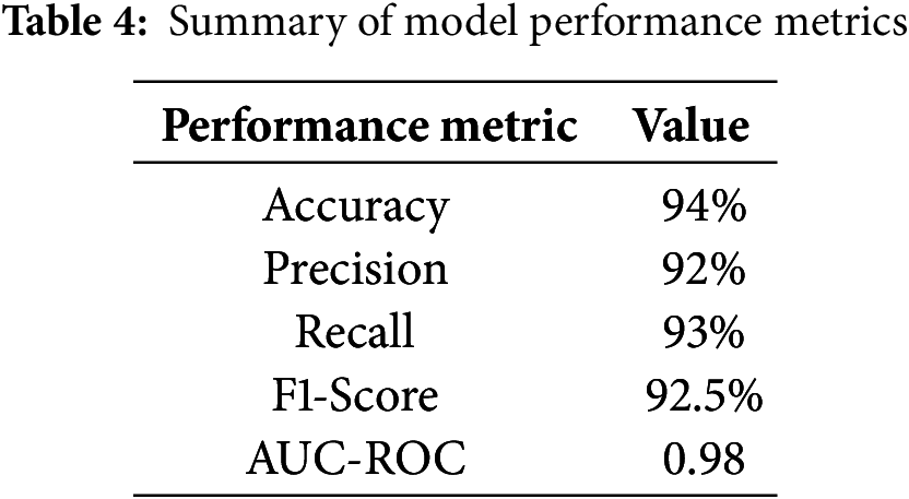
These metrics indicate a high level of performance, suggesting that the model effectively identifies brain tumors from MRI scans. To further contextualize the proposed model’s performance, we compared it against standard models used in medical imaging, such as the original DenseNet without modifications and a basic CNN model, as shown in Table 5.

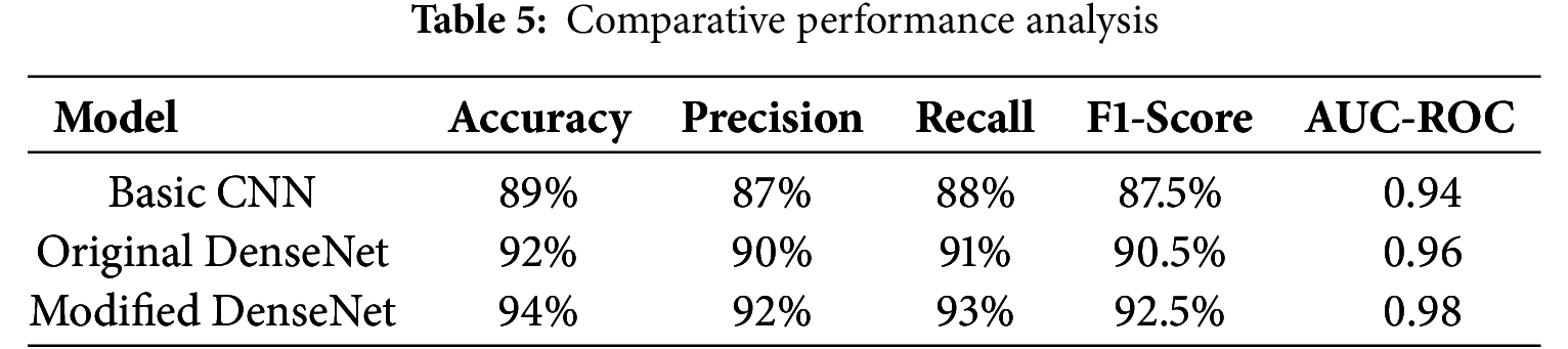
The comparison highlights the enhancements achieved with the modified DenseNet, showing marked improvements in all key metrics. The model’s diagnostic capabilities are illustrated visually in Fig. 4. The proposed DenseNet variant demonstrates consistently higher performance compared to the baseline CNN and standard DenseNet models. The accuracy and AUC-ROC curves indicate faster convergence and reduced performance fluctuations during training, suggesting improved stability of the learning process. In particular, the integration of dilated convolutions enables the network to capture multi-scale contextual features, while the channel-attention mechanism enhances feature selection, both of which contribute to the observed performance gains.

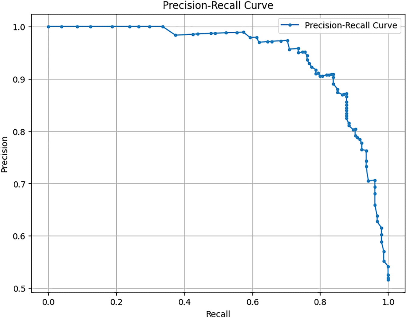
Figure 4: Precision-recall curve

This curve helps visualize the trade-offs between precision and recall for different threshold settings, underlining the robustness of our model in handling various operational scenarios. As shown in Fig. 5 for the model, a confusion matrix gives the real positive and negative, the false positive and negative, which provides an insight into the model working in distinguishing between tumor and non-tumor instances. Some tables give detailed visuals of how the metric of interest, or the threshold, impacted the model’s performance, complementing the other tables presented. This comprehensive evaluation demonstrates that the proposed method of modifying the DenseNet model results in improved performance using standard measures of different machine learning models and still gives significant potential for use in clinical practitioner applications of brain tumor detection.

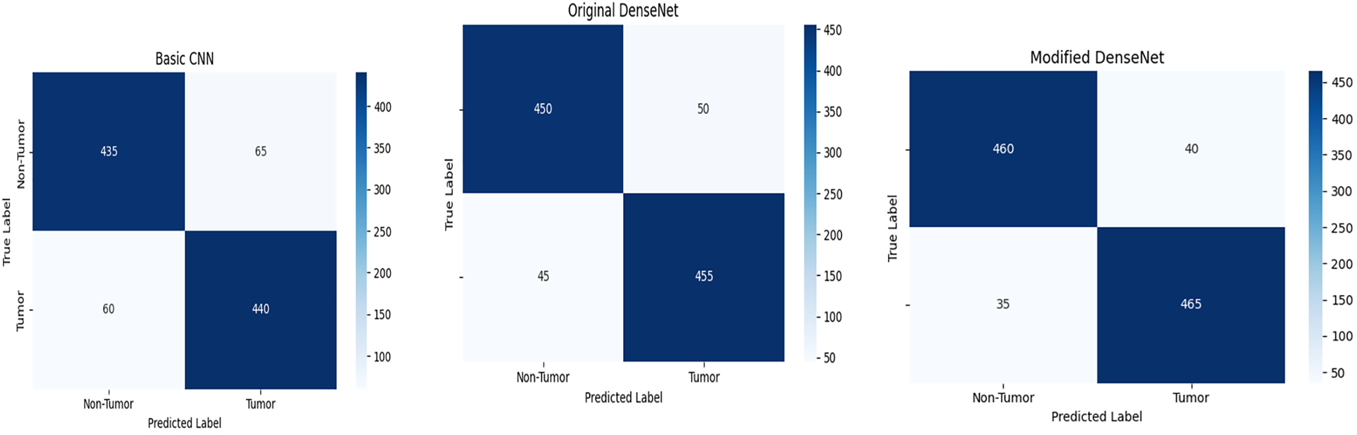
Figure 5: Confusion matrix of basic CNN, original DenseNet, and modified DenseNet

4.3 Interpretability with Grad-CAM Visualizations

Gradient-weighted Class Activation Mapping (Grad-CAM) is used to improve the clarity and reliability of our modified DenseNet model in detecting brain tumors from MRI images. Grad-CAM provides insight into the areas of the image the model should focus on when making predictions and helps define the model’s decision-making process. Grad-CAM creates a coarse localization map by flowing the gradient of each target concept to the final CNN enhancement layer and highlights the required locations in the image to predict the idea. This method is particularly useful in medical imaging to emphasize that model decisions depend on relevant factors in images.

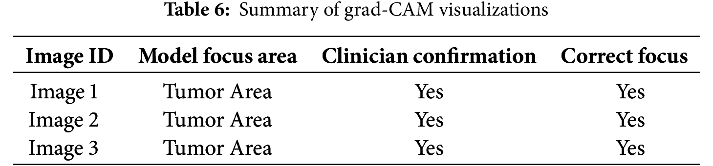
Grad-CAM was applied to the last convolutional layers of the modified DenseNet to visualize the areas of highest activation corresponding to the detection of brain tumors. This helps verify whether the model focuses on the tumor regions rather than non-relevant areas, which is crucial for clinical acceptance. The implementation of Grad-CAM provided clear visual evidence that our model was concentrating on the correct regions in the MRI scans when identifying and classifying tumors. Table 6 indicates that the model’s focus areas aligned with the tumor locations for various test images, as confirmed by clinicians, validating the model’s interpretative ability.

To visually demonstrate how the model processes and interprets MRI images, we present several Grad-CAM heatmaps, as shown in Fig. 6. A heatmap overlay on an MRI image, where the red-to-yellow gradient indicates areas of the highest importance, confirms that the tumor region is correctly identified. Fig. 7 illustrates the heatmaps generated by the basic CNN, the original DenseNet, and our modified DenseNet, highlighting the improved focus and clarity of our model. Fig. 8 shows a more detailed heatmap for MRI images, where tumors are not easily defined or are located in abnormal areas, illustrating how the model performs under stress.

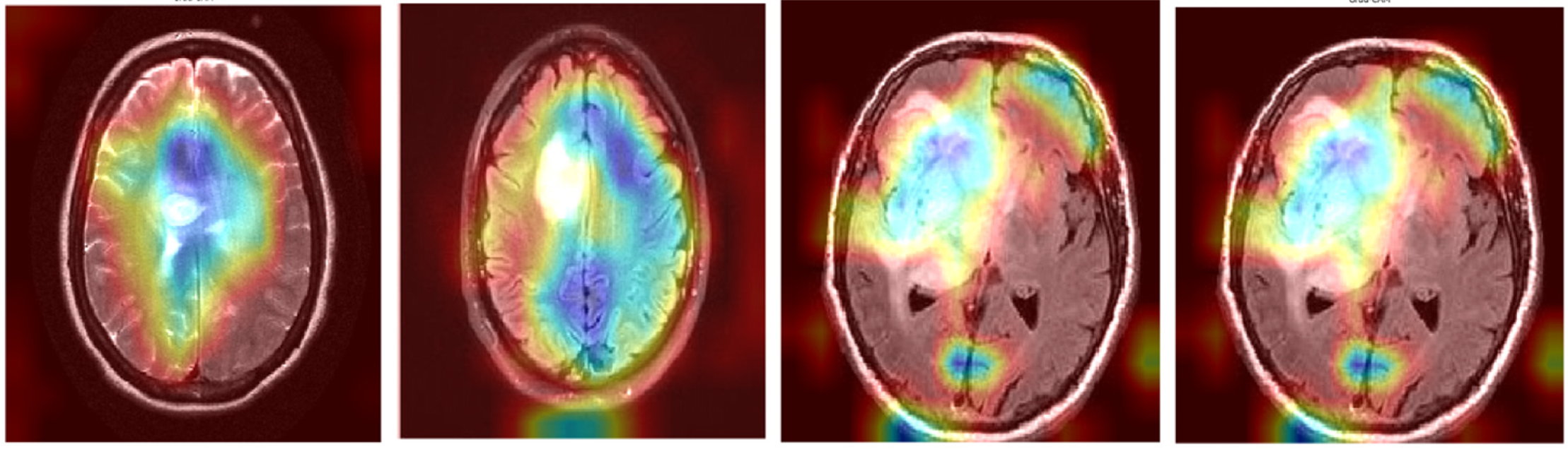
Figure 6: Grad-CAM visualization on a typical tumor MRI

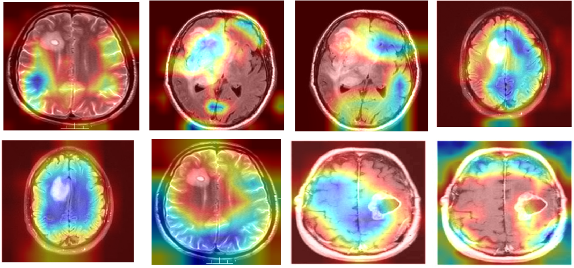
Figure 7: Comparison of grad-CAM heatmaps across different models

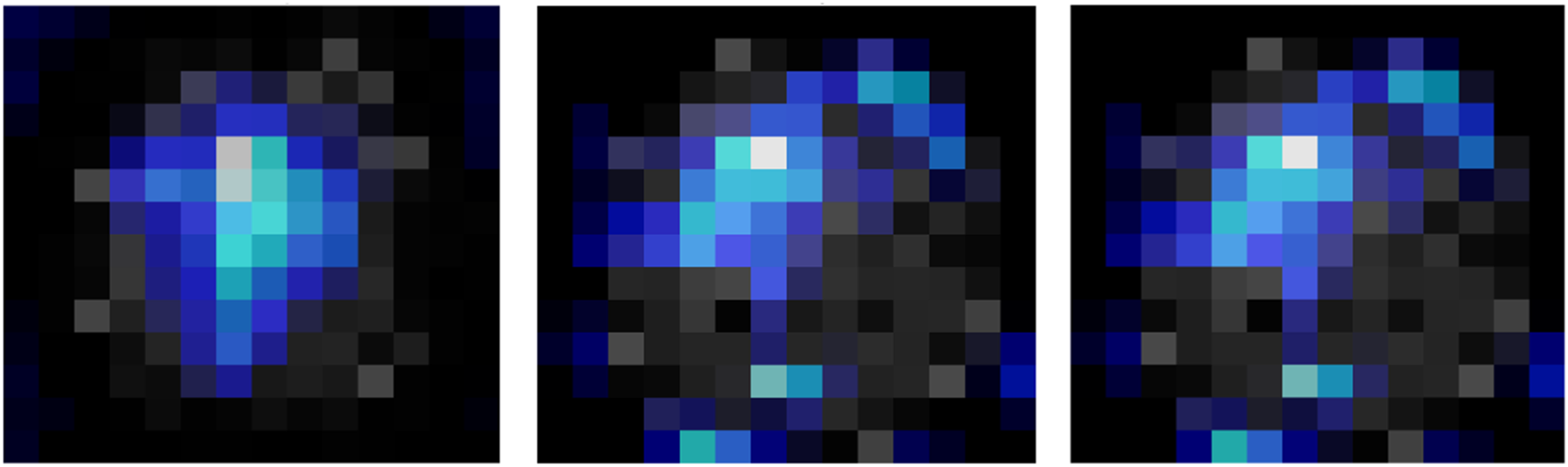
Figure 8: Grad-CAM visualization on edge case scenarios

Fig. 9 illustrates the working of the model to give focus on the tumor region, justifying its diagnostic ability. These Grad-CAM heat map zoning convincingly show that the model draws its predictions from relevant parts of the pattern suitable for diagnosis. It presents a simplified and comprehensible format through which the model’s actions can be easily explained to medical practitioners, thereby motivating clinical integration. Table 7 presents the results of an ablation study analyzing the impact of different architectural modifications on the DenseNet model’s performance.

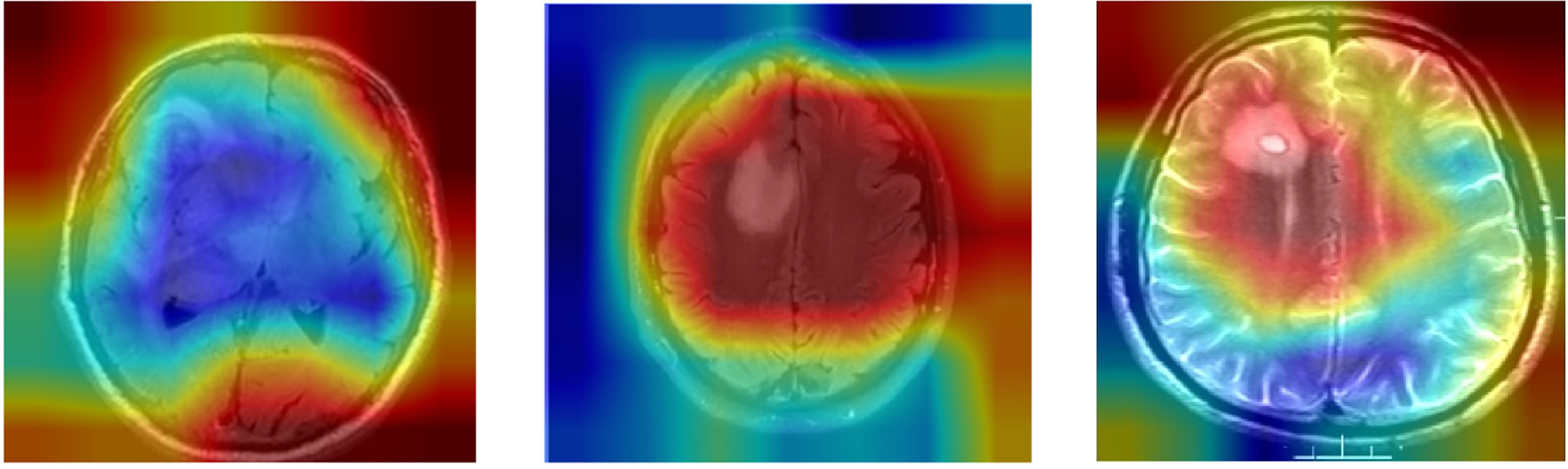
Figure 9: Grad-CAM heatmap for modified DenseNet on MRI image

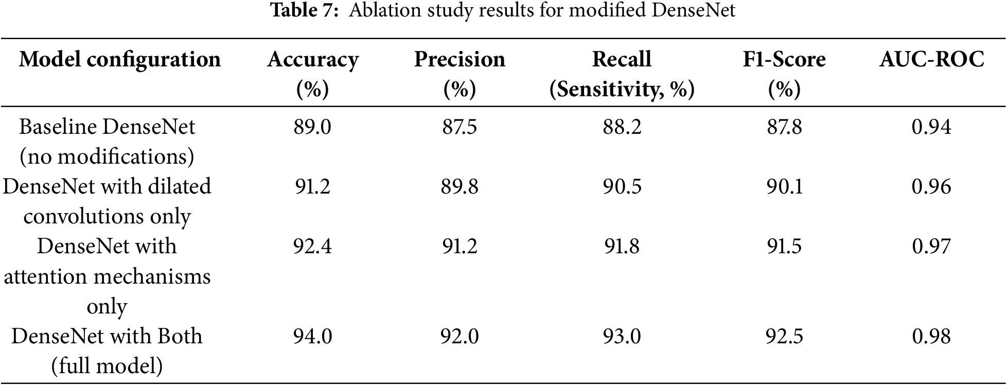
The baseline DenseNet, without any modifications, achieved an accuracy of 89.0% and an AUC-ROC of 0.94. Introducing dilated convolutions improved the accuracy to 91.2% and the AUC-ROC to 0.96, showcasing better spatial detail capture. Adding attention mechanisms enhanced accuracy to 92.4% and AUC-ROC to 0.97 by improving focus on critical tumor regions. The complete model, integrating dilated convolutions and attention mechanisms, achieved the highest performance, with an accuracy of 94.0% and an AUC-ROC of 0.98, demonstrating the synergistic effect of these enhancements.

4.4 Performance Comparison with State-of-the-Art Models

The results were subjected to benchmarking tests against several other state-of-the-art deep learning models to evaluate the proposed modified DenseNet architecture for detecting brain tumors in MR images. This section compares performance variables and variables within the framework, presenting interpretive visuals. All models were evaluated on the following five key performance measures: accuracy, precision, recall, F1 score, and AUC-ROC. Table 8 also reaffirms that our proposed DenseNet, with the applied modifications, is undoubtedly superior to the basic CNN and the original DenseNet in all measured performance metrics, demonstrating its superiority for this particular task.

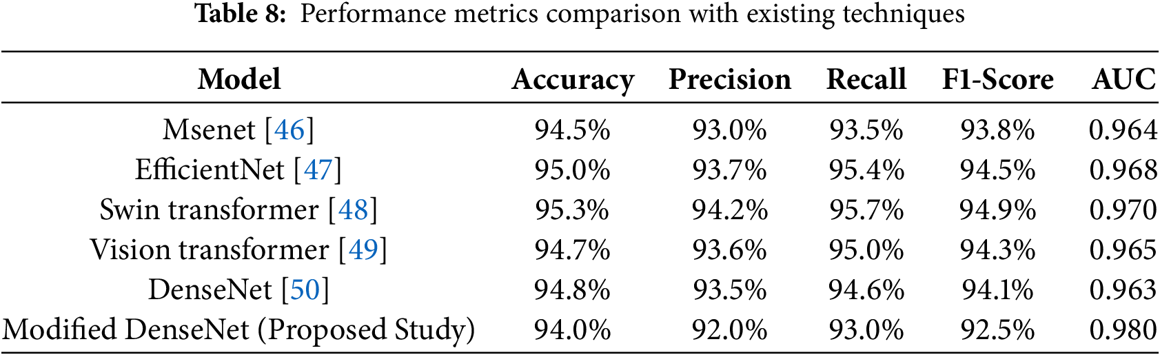
Table 8 compares the performance of our modified DenseNet model in MRI-based brain tumor detection with that of recent state-of-the-art approaches. While techniques like the EfficientNet and Swin Transformer models achieve high accuracy and AUC, our modified DenseNet demonstrates competitive results, achieving 94.0% accuracy and a high AUC of 0.980. These results highlight the model’s effectiveness, particularly in striking a balance between precision and recall, demonstrating its robustness as a reliable tool for tumor identification in MRI scans. The comparisons shown here demonstrate that the changes made to the DenseNet structure significantly improve its performance in MRI images of brain tumors. The synthesized visualization and tabulated comparison support quantitative and qualitative arguments on the effectiveness of our proposed model over regular CNN and DenseNet architectures.

In the literature, we found that a lightweight deep learning based brain tumor model was proposed in [51] and a multilevel brain tumor segmentation model was presented in [52]. In the future, we will enhance our work by comparing it with this research.

5  Conclusion and Future Work

An extension of DenseNet, incorporating dilated convolution and channel attention, was proposed for brain tumor classification using MRI images. Dilated convolutions were introduced to increase the receptive field and extract multi-scale features of the context. Channel attention was utilized to enhance feature selection, resulting in steady improvements in predictive performance. An experimental analysis of the BraTS 2020 dataset yielded 94% accuracy and an AUC of 0.98, outperforming baseline CNN and standard DenseNet models, and achieving similar accuracy to transformer-based and neural architecture search models. The given model provided a good trade-off between accuracy, efficiency, and interpretability, although other advanced architectures offered slightly higher raw accuracy.

Visualization methods like Gradient-weighted Class Activation Mapping (Grad-CAM and SHAP) were more likely to identify model focus with areas of tumor and improve transparency and clinical applicability. Although there are these strengths, there are a few limitations. Validation was performed only for BraTS 2020, and generalizability across BraTS 2018, BraTS 2019, and private multi-center data was not tested. A systematic investigation is also necessary to achieve robustness against variability in acquisition values, scanner variations, and intensity distortion. Moreover, it is still challenging to detect small tumors and accurately define tumor edges.

Future studies ought to expand the validation on various public and private datasets, investigate the level of resistance to domain changes and variability in acquisition, and consider how to combine it with segmentation models to achieve better localization of boundaries and sensitivity to small tumors. One should also focus on computational efficiency, real-time viability in MRI processes and clinical assessment based on radiologist feedback. A variant of DenseNet, utilizing dilated convolutions and channel attention, presents a promising avenue for accurate, interpretable, and efficient brain tumor classification. It may become a valuable tool to support clinical decision-making in neuro-oncology when validated on larger and more diverse datasets.

Acknowledgement: Not applicable.

Funding Statement: This research is supported by the European University of Atlantic.

Author Contributions: The authors confirm contribution to the paper as follows: Conceptualization, Abdu Salam and Farhan Amin; methodology, Mohammad Abrar; software, Raja Waseem Anwer; validation, Faizan Ullah, Isabel de la Torre and Farhan Amin; formal analysis, Faizan Ullah; investigation, Mohammad Abrar; resources, Gerardo Mendez Mezquita; data curation, Henry Fabian Gongora; writing—original draft preparation, Isabel de la Torre, Farhan Amin and Abdu Salam; writing—review and editing, Farhan Amin; visualization, Farhan Amin; supervision, Farhan Amin; project administration, Isabel de la Torre; funding acquisition, Isabel de la Torre. All authors reviewed the results and approved the final version of the manuscript.

Availability of Data and Materials: BRATS-2020, Kaggle, 2020 [Online]. Available at: https://www.med.upenn.edu/cbica/brats2020/data.html (accessed on 10 October 2025).

Ethics Approval: Not applicable.

Conflicts of Interest: The authors declare no conflicts of interest to report regarding the present study.

References

1. Gritsch S, Batchelor TT, Gonzalez Castro LN. Diagnostic, therapeutic, and prognostic implications of the 2021 World Health Organization classification of tumors of the central nervous system. Cancer. 2022;128(1):47–58. doi:10.1002/cncr.33918. [Google Scholar] [PubMed] [CrossRef]

2. Cacho-Díaz B, García-Botello DR, Wegman-Ostrosky T, Reyes-Soto G, Ortiz-Sánchez E, Herrera-Montalvo LA. Tumor microenvironment differences between primary tumor and brain metastases. J Transl Med. 2020;18(1):1. doi:10.1186/s12967-019-02189-8. [Google Scholar] [PubMed] [CrossRef]

3. Ghandour F, Squassina A, Karaky R, Diab-Assaf M, Fadda P, Pisanu C. Presenting psychiatric and neurological symptoms and signs of brain tumors before diagnosis: a systematic review. Brain Sci. 2021;11(3):301. doi:10.3390/brainsci11030301. [Google Scholar] [PubMed] [CrossRef]

4. Dandil E, Biçer A. Automatic grading of brain tumours using LSTM neural networks on magnetic resonance spectroscopy signals. IET Image Process. 2020;14(10):1967–79. doi:10.1049/iet-ipr.2019.1416. [Google Scholar] [CrossRef]

5. Abdusalomov AB, Mukhiddinov M, Whangbo TK. Brain tumor detection based on deep learning approaches and magnetic resonance imaging. Cancers. 2023;15(16):4172. doi:10.3390/cancers15164172. [Google Scholar] [PubMed] [CrossRef]

6. Huang J, Shlobin NA, Lam SK, DeCuypere M. Artificial intelligence applications in pediatric brain tumor imaging: a systematic review. World Neurosurg. 2022;157:99–105. doi:10.1016/j.wneu.2021.10.068. [Google Scholar] [PubMed] [CrossRef]

7. Forghani R. Precision digital oncology: emerging role of radiomics-based biomarkers and artificial intelligence for advanced imaging and characterization of brain tumors. Radiol Imaging Cancer. 2020;2(4):e190047. doi:10.1148/rycan.2020190047. [Google Scholar] [PubMed] [CrossRef]

8. Rao CS, Karunakara K. A comprehensive review on brain tumor segmentation and classification of MRI images. Multimed Tools Appl. 2021;80(12):17611–43. doi:10.1007/s11042-020-10443-1. [Google Scholar] [CrossRef]

9. Martucci M, Russo R, Schimperna F, D’Apolito G, Panfili M, Grimaldi A, et al. Magnetic resonance imaging of primary adult brain tumors: state of the art and future perspectives. Biomedicines. 2023;11(2):364. doi:10.3390/biomedicines11020364. [Google Scholar] [PubMed] [CrossRef]

10. Scola E, Del Vecchio G, Busto G, Bianchi A, Desideri I, Gadda D, et al. Conventional and advanced magnetic resonance imaging assessment of non-enhancing peritumoral area in brain tumor. Cancers. 2023;15(11):2992. doi:10.3390/cancers15112992. [Google Scholar] [PubMed] [CrossRef]

11. Bastiancich C, Malfanti A, Préat V, Rahman R. Rationally designed drug delivery systems for the local treatment of resected glioblastoma. Adv Drug Deliv Rev. 2021;177:113951. doi:10.1016/j.addr.2021.113951. [Google Scholar] [PubMed] [CrossRef]

12. Manan HA, Franz EA, Yahya N. Functional connectivity changes in patients with brain tumours—a systematic review on resting state-fMRI. Neurol Psychiatry Brain Res. 2020;36:73–82. doi:10.1016/j.npbr.2020.03.003. [Google Scholar] [CrossRef]

13. Weinberg BD, Kuruva M, Shim H, Mullins ME. Clinical applications of magnetic resonance spectroscopy in brain tumors: from diagnosis to treatment. Radiol Clin North Am. 2021;59(3):349–62. doi:10.1016/j.rcl.2021.01.004. [Google Scholar] [PubMed] [CrossRef]

14. Hu R, Hoch MJ. Application of diffusion weighted imaging and diffusion tensor imaging in the pretreatment and post-treatment of brain tumor. Radiol Clin North Am. 2021;59(3):335–47. doi:10.1016/j.rcl.2021.01.003. [Google Scholar] [PubMed] [CrossRef]

15. Arnold TC, Freeman CW, Litt B, Stein JM. Low-field MRI: clinical promise and challenges. Magn Reson Imaging. 2023;57(1):25–44. doi:10.1002/jmri.28408. [Google Scholar] [PubMed] [CrossRef]

16. Cè M, Irmici G, Foschini C, Danesini GM, Falsitta LV, Serio ML, et al. Artificial intelligence in brain tumor imaging: a step toward personalized medicine. Curr Oncol. 2023;30(3):2673–701. doi:10.3390/curroncol30030203. [Google Scholar] [PubMed] [CrossRef]

17. Sarvamangala DR, Kulkarni RV. Convolutional neural networks in medical image understanding: a survey. Evol Intell. 2022;15(1):1–22. doi:10.1007/s12065-020-00540-3. [Google Scholar] [PubMed] [CrossRef]

18. Krizhevsky A, Sutskever I, Hinton GE. Imagenet classification with deep convolutional neural networks. Adv Neural Inf Process Syst. 2012;25:1–9. doi:10.1145/3065386. [Google Scholar] [CrossRef]

19. Singh N, Sabrol H. Convolutional neural networks-an extensive arena of deep learning. a comprehensive study. Arch Comput Meth Eng. 2021;28(7):4755–80. doi:10.1007/s11831-021-09551-4. [Google Scholar] [CrossRef]

20. McNeely-White D, Beveridge JR, Draper BA. Inception and ResNet features are (almost) equivalent. Cogn Syst Res. 2020;59:312–8. doi:10.1016/j.cogsys.2019.10.004. [Google Scholar] [CrossRef]

21. Yin H, Vahdat A, Alvarez JM, Mallya A, Kautz J, Molchanov P. A-ViT: adaptive tokens for efficient vision transformer. In: 2022 IEEE/CVF Conference on Computer Vision and Pattern Recognition (CVPR); 2022 Jun 18–24; New Orleans, LA, USA. p. 10799–808. doi:10.1109/CVPR52688.2022.01054. [Google Scholar] [CrossRef]

22. Overcast WB, Davis KM, Ho CY, Hutchins GD, Green MA, Graner BD, et al. Advanced imaging techniques for neuro-oncologic tumor diagnosis, with an emphasis on PET-MRI imaging of malignant brain tumors. Curr Oncol Rep. 2021;23(3):34. doi:10.1007/s11912-021-01020-2. [Google Scholar] [PubMed] [CrossRef]

23. Zhou SK, Greenspan H, Davatzikos C, Duncan JS, Van Ginneken B, Madabhushi A, et al. A review of deep learning in medical imaging: imaging traits, technology trends, case studies with progress highlights, and future promises. Proc IEEE. 2021;109(5):820–38. doi:10.1109/JPROC.2021.3054390. [Google Scholar] [PubMed] [CrossRef]

24. Sadad T, Rehman A, Munir A, Saba T, Tariq U, Ayesha N, et al. Brain tumor detection and multi-classification using advanced deep learning techniques. Microsc Res Tech. 2021;84(6):1296–308. doi:10.1002/jemt.23688. [Google Scholar] [PubMed] [CrossRef]

25. Woźniak M, Siłka J, Wieczorek M. Deep neural network correlation learning mechanism for CT brain tumor detection. Neural Comput Appl. 2023;35(20):14611–26. doi:10.1007/s00521-021-05841-x. [Google Scholar] [CrossRef]

26. Ullah F, Nadeem M, Abrar M. Revolutionizing brain tumor segmentation in MRI with dynamic fusion of handcrafted features and global pathway-based deep learning. KSII Trans Internet Inf Syst. 2024;18(1):105–25. doi:10.3837/tiis.2024.01.007. [Google Scholar] [CrossRef]

27. Louis DN, Perry A, Wesseling P, Brat DJ, Cree IA, Figarella-Branger D, et al. The 2021 WHO classification of tumors of the central nervous system: a summary. Neuro Oncol. 2021;23(8):1231–51. doi:10.1093/neuonc/noab106. [Google Scholar] [PubMed] [CrossRef]

28. Malik V, Mittal R, Rana A, Khan I, Singh P, Alam B. Coronary heart disease prediction using GKFCM with RNN. In: 2023 6th International Conference on Contemporary Computing and Informatics (IC3I); 2023 Sep 14–16; Gautam Buddha Nagar, India. p. 677–82. doi:10.1109/IC3I59117.2023.10398020. [Google Scholar] [CrossRef]

29. Thust SC, van den Bent MJ, Smits M. Pseudoprogression of brain tumors. Magn Reson Imaging. 2018;48(3):571–89. doi:10.1002/jmri.26171. [Google Scholar] [PubMed] [CrossRef]

30. Tajbakhsh N, Shin JY, Gurudu SR, Hurst RT, Kendall CB, Gotway MB, et al. Convolutional neural networks for medical image analysis: full training or fine tuning? IEEE Trans Med Imag. 2016;35(5):1299–312. doi:10.1109/TMI.2016.2535302. [Google Scholar] [PubMed] [CrossRef]

31. Baur C, Albarqouni S, Navab N. Semi-supervised deep learning for fully convolutional networks. In: International Conference on Medical Image Computing and Computer Assisted Intervention; 2017 Sep 11–13; Quebec City, QC, Canada. p. 311–9. doi:10.1007/978-3-319-66179-7_36. [Google Scholar] [CrossRef]

32. Castelvecchi D. Can we open the black box of AI? Nature. 2016;538(7623):20–3. doi:10.1038/538020a. [Google Scholar] [PubMed] [CrossRef]

33. Cheplygina V, de Bruijne M, Pluim JPW. Not-so-supervised: a survey of semi-supervised, multi-instance, and transfer learning in medical image analysis. Med Image Anal. 2019;54(1):280–96. doi:10.1016/j.media.2019.03.009. [Google Scholar] [PubMed] [CrossRef]

34. Zech JR, Badgeley MA, Liu M, Costa AB, Titano JJ, Oermann EK. Variable generalization performance of a deep learning model to detect pneumonia in chest radiographs: a cross-sectional study. PLoS Med. 2018;15(11):e1002683. doi:10.1371/journal.pmed.1002683. [Google Scholar] [PubMed] [CrossRef]

35. Goriparthi RG. Interpretable machine learning models for healthcare diagnostics: addressing the Black-Box problem. Rev De Intel Artif En Med. 2022;13(1):508–34. [Google Scholar]

36. Holzinger A, Malle B, Kieseberg P, Roth PM, Müller H, Reihs R, et al. Towards the augmented pathologist: challenges of explainable-ai in digital pathology. arXiv:1712.06657. 2017. [Google Scholar]

37. Gulshan V, Peng L, Coram M, Stumpe MC, Wu D, Narayanaswamy A, et al. Development and validation of a deep learning algorithm for detection of diabetic retinopathy in retinal fundus photographs. JAMA. 2016;316(22):2402–10. doi:10.1001/jama.2016.17216. [Google Scholar] [PubMed] [CrossRef]

38. Char DS, Shah NH, Magnus D. Implementing machine learning in health care—addressing ethical challenges. N Engl J Med. 2018;378(11):981–3. doi:10.1056/nejmp1714229. [Google Scholar] [PubMed] [CrossRef]

39. Jiang F, Jiang Y, Zhi H, Dong Y, Li H, Ma S, et al. Artificial intelligence in healthcare: past, present and future. Stroke Vasc Neurol. 2017;2(4):230–43. doi:10.1136/svn-2017-000101. [Google Scholar] [PubMed] [CrossRef]

40. Khan MBS, Atta-ur-Rahman, Nawaz MS, Ahmed R, Khan MA, Mosavi A. Intelligent breast cancer diagnostic system empowered by deep extreme gradient descent optimization. Math Biosci Eng. 2022;19(8):7978–8002. doi:10.3934/mbe.2022373. [Google Scholar] [PubMed] [CrossRef]

41. Siddiqui SY, Haider A, Ghazal TM, Khan MA, Naseer I, Abbas S, et al. IoMT cloud-based intelligent prediction of breast cancer stages empowered with deep learning. IEEE Access. 2021;9:146478–91. doi:10.1109/ACCESS.2021.3123472. [Google Scholar] [CrossRef]

42. Hasan N, Rana MM, Hasan MM, Azad A, Afroz D, Komol MMR, et al. STSA-based early-stage detection of small brain tumors using neural network. Eng Rep. 2025;7(5):e70135. doi:10.1002/eng2.70135. [Google Scholar] [CrossRef]

43. Hasan MS, Komol MMR, Fahim F, Islam J, Pervin T, Hasan MM. DEEP Q-NAS: a new algorithm based on neural architecture search and reinforcement learning for brain tumor identification from MRI. Comput Biol Med. 2025;196(Pt B):110767. doi:10.1016/j.compbiomed.2025.110767. [Google Scholar] [PubMed] [CrossRef]

44. Zhu Y, Newsam S. DenseNet for dense flow. In: 2017 IEEE International Conference on Image Processing (ICIP); 2017 Sep 17–20; Beijing, China. p. 790–4. doi:10.1109/ICIP.2017.8296389. [Google Scholar] [CrossRef]

45. BRATS-2020. Kaggle 2020 [Online]. [cited 2025 Jan 1]. Available from: https://www.med.upenn.edu/cbica/brats2020/data.html. [Google Scholar]

46. Bodapati JD, Shareef SN, Naralasetti V, Mundukur NB. MSENet: multi-modal squeeze-and-excitation network for brain tumor severity prediction. Int J Patt Recogn Artif Intell. 2021;35(7):2157005. doi:10.1142/s0218001421570056. [Google Scholar] [CrossRef]

47. Ali Shah H, Saeed F, Yun S, Park JH, Paul A, Kang JM. A robust approach for brain tumor detection in magnetic resonance images using finetuned EfficientNet. IEEE Access. 2022;10:65426–38. doi:10.1109/ACCESS.2022.3184113. [Google Scholar] [CrossRef]

48. Jiang Y, Zhang Y, Lin X, Dong J, Cheng T, Liang J. SwinBTS: a method for 3D multimodal brain tumor segmentation using swin transformer. Brain Sci. 2022;12(6):797. doi:10.3390/brainsci12060797. [Google Scholar] [PubMed] [CrossRef]

49. Tummala S, Kadry S, Ahmad Chan Bukhari S, Rauf HT. Classification of brain tumor from magnetic resonance imaging using vision transformers ensembling. Curr Oncol. 2022;29(10):7498–511. doi:10.3390/curroncol29100590. [Google Scholar] [PubMed] [CrossRef]

50. Jean S. A pretrained DenseNet encoder for brain tumor segmentation. In: International MICCAI Brainlesion Workshop; 2018 Sep 16; Granada, Spain. p. 105–15. doi:10.1007/978-3-030-11726-9_10. [Google Scholar] [CrossRef]

51. Rahman MA, Masum MI, Hasib KM, Mridha MF, Alfarhood S, Safran M, et al. GliomaCNN: an effective lightweight CNN model in assessment of classifying brain tumor from magnetic resonance images using explainable AI. Comput Model Eng Sci. 2024;140(3):2425–48. doi:10.32604/cmes.2024.050760. [Google Scholar] [CrossRef]

52. Tie J, Peng H. Multi-level parallel network for brain tumor segmentation. Comput Model Eng Sci. 2024;139(1):741–57. doi:10.32604/cmes.2023.043353. [Google Scholar] [CrossRef]