Three-Dimensional Hybrid Model for Wave Interaction with Porous Layer

1  Introduction

Wave-porous structure interaction is a critical area of study in coastal and ocean engineering, particularly in the design and analysis of coastal defenses such as breakwaters, submerged reefs, and other protective barriers. These porous structures typically composed of materials like rocks, concrete, or geotextiles and play a vital role in mitigating the impact of waves on shorelines, ports, and offshore installations. Understanding the wave interaction with porous media is essential for predicting the effectiveness in reducing wave energy, controlling erosion, and maintaining the stability of coastal environments. The interaction between waves and porous structures is a complex phenomenon that involves the transfer of energy, momentum, and mass between the fluid (wave) and the solid (porous structure). The presence of porosity within the structure introduces additional factors such as drag forces, wave attenuation, and dissipation, which must be accounted in the modeling and analysis of wave dynamics. These effects can significantly alter wave propagation, reduce wave height, and influence the wave-induced forces on the structure itself. Advanced computational models that combine fluid dynamics with porous media properties are essential for accurately capturing these interactions. Such models allow for a better understanding of the fluid flow through the porous material, the resistance it generates, and its impact on wave behavior. This knowledge is crucial for optimizing the design of coastal protection systems, ensuring their effectiveness, durability, and resilience to extreme wave events.

Numerical modeling of wave-porous structure interactions can be approached at either the microscopic or macroscopic scale. The microscopic approach involves modeling individual soil particles and analyzing the interaction of the wave with each particle. While this method can be accurate, it is computationally expensive and time-consuming. In contrast, the macroscopic model treats the porous structure as a whole, where wave energy is dissipated due to the collective drag forces of the soil particles. Although this approach may not provide precise force calculations on each individual particle, it allows for faster analysis of wave attenuation. This study focuses on wave attenuation, and therefore, the macroscopic model is used. The developed macroscopic model can be either mesh-based or meshless. In mesh-based approaches for wave–porous structure interactions, various numerical techniques have been adopted. The Finite Element Method was applied in [1], the Finite Difference Method in [2], and the Finite Analytic Method in [3]. A two-phase (fluid–air) model based on the Volume of Fluid (VOF) method was developed in [4]. The model proposed in [5] was enhanced by [6] using the VOF method to simulate wave overtopping of rubble-mound breakwaters. Applications of OpenFOAM in wave–structure interactions, including breakwater and scour modeling, are discussed in [7].

Several three-dimensional (3D) models have also been developed. For instance, Ref. [8] investigated dam-break wave interactions with porous structures using 3D volume-averaged Navier–Stokes (VANS) equations, incorporating turbulence through Large Eddy Simulation (LES). In [9], the VARANS equations were re-derived via a volume-averaging process, and the porous resistance coefficients were calibrated for dam-break cases. Subsequently, Ref. [10] developed the IHFOAM model, which solves the VARANS equations within the open-source framework OpenFOAM. All these models are based on a Eulerian framework.

In Lagrangian framework applications of the SPH method to porous media flows have been predominantly concentrated in civil engineering, particularly within hydraulic and coastal engineering disciplines. This emphasis is largely due to the practical challenges posed by fluid–structure interactions involving permeable coastal defenses and other porous barriers. Such problems are commonly associated with free-surface flows, a context in which SPH has proven to be especially effective. Several studies employing the Weakly Compressible Smoothed Particle Hydrodynamics (WCSPH) approach have significantly advanced research in this field. For instance, the study in [11] investigated the width of the transition zone, while those in [12–16] validated WCSPH formulations for wave–current interactions involving porous media. Furthermore, the work in [17] extended the WCSPH method to simulate turbulent free-surface channel flows over porous gravel beds. In the context of turbulence modeling within SPH, the Sub-Particle Scale (SPS) approach is most commonly adopted, with occasional use of the k–ε model. The SPS method accounts for unresolved sub-grid-scale stresses at the particle level by employing an empirical model that relates these stresses to macroscopic flow variables [18–21]. In contrast, the k–ε model adopts a more complex framework involving transport equations for turbulent kinetic energy (k) and its dissipation rate (ε), but its performance is often sensitive to the calibration of several empirical constants [22–25]. Nevertheless, despite these developments, turbulence modeling within WCSPH still faces challenges, particularly in capturing flow behavior near porous boundaries, indicating the need for continued refinement and validation of existing models.

Parallel developments have also been made using incompressible SPH (ISPH) and moving particle semi-implicit (MPS) methods. These approaches, reported in studies such as [26–28] have been widely applied in coastal flow problems. Unlike WCSPH, ISPH and MPS solve Poisson’s equation to implicitly determine pressure, thereby yielding more accurate pressure fields—a key factor for resolving velocity and force distributions. However, these schemes are not without difficulties: configuring particle discretization so that the porous region has coarser spacing than the surrounding free-flow domain remains problematic. The abrupt change in resolution often induces spurious pressure oscillations near the interface, complicating numerical stability. Ref. [29] has reviewed all the available methods for wave porous structure interaction where the study concludes that the macroscopic model is well suited for coastal problems.

In our previous study [30], a two-dimensional wave–porous interaction model was developed using IMLPG_R, which demonstrated satisfactory performance. Similarly, Ref. [31] proposed a modified moving particle method that incorporated turbulence effects at the interface zone. Their findings showed that sharp velocity gradients at the interface can induce small turbulent jets, which were addressed through the implementation of a sub-particle scale (SPS) turbulence model to improve accuracy. In contrast, the present study extends our earlier work [30] by modeling the interface with a smooth velocity transition achieved through linearly varying porosity. This treatment reduces steep velocity gradients and suppresses the formation of small turbulent jets, and therefore turbulence effects are neglected in the current formulation. While these studies were primarily limited to two-dimensional cases, Ref. [32] also introduced a hybrid model to investigate wave–structure interactions. However, Lagrangian-based approaches remain relatively rare due to their high computational cost. More recently, Ref. [33] presented a three-dimensional Lattice Boltzmann model for simulating wave interaction with permeable structures with LES incorporated. This study shows the computational efficiency of the developed 3D Lattice Boltzmann method compared to other available SPH models.

In the present study, a hybrid model combining both mesh-based and mesh-free methods is employed to reduce computation time. This approach leverages the strengths of both models, enhancing accuracy. The FNPT model is irrotational and excludes viscous terms, while the 3D IMLPG_R model accounts for viscosity, incorporating additional drag forces from the soil particles. The larger domain is divided into two regions: the FNPT model is used in areas without the structure, and the 3D IMLPG_R model is applied to regions containing the porous structure. A buffer zone is introduced, where field variables from the FNPT model are transferred to the 3D IMLPG_R model. Fig. 1 gives an overview of the hybrid model. Ref. [32] demonstrated the efficiency of this hybrid model in simulating wave interactions with cylinders. This study extends their work by applying the model to wave-porous structure interactions. Ref. [32] shows the developed model for a flat-bottomed bed, which was later extended to include a sloping bottom in our previous study [34]. However, when the sloping bed was introduced, the particle distribution became uneven, and a significant gap appeared between the bottom bed and the fluid as the wave propagated. In our 2D IMLPG_R, the gaps between the particles are addressed using a minimum pressure gradient and interpolation as given in [35]. In 3D IMLPG, Ref. [32] adopted the re-distribution of the nodes. However, for complex geometry, redistribution of the nodes will not be effective. To address this issue, the Particle Shifting Algorithm (PST) was applied.

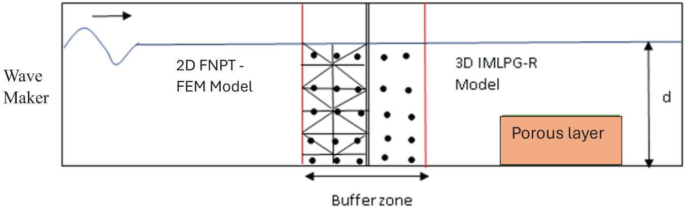
Figure 1: Overview of the hybrid model

The study by [36] developed a PST algorithm for incompressible flows using Smooth Particle Hydrodynamics (SPH), building on the earlier work of [37]. In [38], various PST algorithms were reviewed, and their limitations were highlighted. Some of the reviewed PST algorithms include: the method proposed in [39], where the PST algorithm does not rely on Fick’s law but instead updates particle positions based on the velocity of neighboring particles, with consistency ensured by adding a correction term; and the approach in [37], where the PST algorithm is formulated on the basis of Fick’s law, and a velocity limit is imposed in deriving the concentration gradient. Ref. [40] shows a quasi-Lagrangian shifting where the influence of Mach number comes into picture. Ref. [41] developed a consistent approach of particle shifting which can be applied for compressible flow.

The generalized particle shifting technique proposed in [36] incorporates the dimensionality factor in the diffusion term, enabling seamless application to both two- and three-dimensional flows. Previous PST-based studies were often associated with high computational costs and challenges in selecting appropriate shifting coefficients, many of which were based on Mach number criteria and thus not suitable for the present study. Since the current model assumes incompressible flow, the PST algorithm of [36] was adopted and implemented with modifications to the weighting function and velocity ratio. This method was chosen because it is computationally efficient and provides a systematic approach for selecting shifting vectors, avoiding ad-hoc criteria. The PST algorithm works by redistributing particles from areas of high concentration to regions of lower concentration. This diffusion follows Fick’s law. The developed model along with the PST algorithm is used to validate for single porous layer flow and multi porous layer.

This paper is organized as follows; after the introduction section, the hybrid model is explained giving the governing equation for both 2D FNPT and IMLPG_R in Section 1. Section 2 gives the numerical algorithm followed in 3D IMLPG_R. Section 3 gives the problems caused due to the introduction of sloping bed and the PST algorithm applied. Section 4 gives the validation of developed model for single trapezoidal breakwater and two-layer trapezoidal breakwater. Section 5 gives the further studies done for solitary wave interaction with porous layer.

2  Governing Equation and Boundary Condition

Governing equation for 2D FNPT:

FNPT assumes the fluid to be incompressible, irrotational and inviscid. The governing equation is the 2D Laplacian equation of velocity potential ϕ(x,z,t) and is given in Eq. (1). Here a 2D plane of XZ is used, where Z = 0 at the bottom and goes positive in the vertical direction.

∂2ϕ∂x2+∂2ϕ∂z2=0(1)

The left boundary Гw of the 2D domain is the wave maker. Neumann boundary condition given in Eq. (2a) is applied on the boundary Гw. The bottom Гb and the right boundary Гr has the condition given in Eq. (2b). Free surface Гf is assumed to be non-breaking and with non-linear dynamic free surface boundary condition derived from Bernoullis equation as given in Eq. (2c).

∂ϕ∂x=xp˙(t)at x=xp˙(t) onΓw(2a)

∂ϕ∂n=0onΓb andΓr(2b)

∂ϕ∂t=−gη−12∇ϕ∇ϕonΓf(2c)

where xp˙(t) is the wave probe velocity, g is the acceleration due to gravity and η is the free surface elevation. The initial condition is assumed as η=0 at time t = 0. Solution for this problem is obtained using Finite element method (FEM) with structured triangular mesh which has a variable spacing along the water depth. Ref. [42] explains the further details of this numerical model. An absorption layer is implemented upstream of the right boundary wall to attenuate the propagating wave and prevent reflections. In the present model, the length of the absorption layer is typically set to three times the wavelength of the incoming wave [43].

Governing equation for 3D IMLPG_R:

The governing formulation for three-dimensional porous flow within the IMLPG_R framework was originally established in the seminal work of [44], where the pressure gradient was demonstrated to vary linearly with the flow velocity through the introduction of the permeability coefficient—indicating that higher permeability facilitates greater fluid motion within the porous domain. Darcy’s law, which embodies this linear relationship, is applicable primarily to laminar flows characterized by low permeability. To extend its applicability to turbulent regimes, Ref. [45] incorporated a nonlinear drag term, wherein the resistance force varies with the square of the fluid velocity. Subsequently, Ref. [46] enhanced the model by including a virtual mass coefficient in the local acceleration term to account for added inertia effects.

In the context of wave–porous structure interactions, the resulting governing equations incorporate additional resistance components: a linear drag term representing laminar flow, a nonlinear drag term corresponding to turbulent flow, and a virtual mass term for inertial effects. The momentum equation thus attains a unified form, encompassing both linear and nonlinear drag contributions as expressed in Eq. (4). Following the approach proposed in [26], this formulation is implemented within a Lagrangian framework, wherein a single governing equation is applied seamlessly across both fluid and porous regions, with porosity serving as the distinguishing variable. The three-dimension model is based on Cartessian coordinates of OXYZ with Z = 0 and goes positive in the vertical direction. The velocity vector in three dimension is given as u→D=uDi^+vDj^+wDk^

∇⋅u→D=0(3)

Crnw⋅Du→DDt=−1ρw∇→P+ϑeff∇2u→D−au→D−bu→D|u→D|(4)

here, Cr denotes the inertia coefficient, nw represents the porosity, P is the pressure, and υeff corresponds to the effective viscosity as defined by Brinkman [47]. The coefficients a and b signify the linear and nonlinear drag terms, respectively, while g and ρw denote the gravitational acceleration and fluid density. This formulation provides a unified governing equation applicable to the entire computational domain, thereby eliminating the need for explicit interface treatment between the fluid and porous regions.

u→D=nwu→f(5)

ϑeff=ϑnw(6)

In this context, υ denotes the kinematic viscosity. The pressure at the free surface is considered to be zero (P = 0). The kinematic boundary condition, expressed in Lagrangian form, is given by dr→dt=u→f, where r→ represents the position vector and u→f denotes the velocity vector of the fluid particle.

On solid boundary, the following condition has to be satisfied,

n→⋅u→D=n→⋅U→D(7)

n→⋅∇P=ρw⋅n→(ϑeff∇2u→D−a⋅u→D−b⋅u→D|u→D|+g→−U˙→D⋅Crnw)(8)

here, U˙→D denotes the acceleration of the solid boundary, and U→D represents its velocity. The linear and nonlinear drag coefficients, a and b, are functions of the Reynolds number and the prevailing flow regime. The linear drag component predominates under laminar conditions, whereas the nonlinear term becomes significant in turbulent flows. The generalized expressions for these coefficients are presented below, wherein the exponents k, m, and n vary depending on experimental observations reported in [48].

a=αϑw(1−nw)knwmD50nb=β1−nwnw3D50Cr=1+1−nwnwγ with γ=0.34(9)

3  Numerical Algorithm and Hybrid Model Layout

The governing equation, together with the associated boundary conditions, is solved using the time-splitting algorithm proposed by Chorin [49], as detailed below,

(a) Compute the intermediate velocity by neglecting the pressure term in Eq. (4), yielding:

u→D∗=u→Dn+nw∗dtcr[ϑeff∇2u→D−au→D−bu→D|u→D|](10)

x*=xn+uD∗dt(11a)

y*=yn+vD∗dt(11b)

z*=zn+wD∗dt(11c)

(b) The Pressure Poisson Equation (PPE) is solved using the intermediate velocity within a semi-implicit framework.

∇2Pn+1=cr∗ρwdt∗nw⋅∇u→D∗(12)

(c) The pressure gradient at the n+1 time step is then employed to compute the Darcy velocity at the same step.

u→D∗∗=−dt∗nwρw∗cr∇Pn+1(13)

u→Dn+1=u→D∗−dt∗nwρw∗cr∇Pn+1+g→⋅dt(14)

(d) Utilizing the Darcy velocity, the fluid particle velocities uf, vf and wf in X, Y and Z directions, respectively, are determined from Eq. (4), after which the position vectors are updated accordingly based on the computed fluid velocities.

ufn+1=uDn+1nw;vfn+1=vDn+1nw;wfn+1=wDn+1nw(15)

xn+1=xn+ufn+1dt;yn+1=yn+vfn+1dt;zn+1=zn+wfn+1dt(16)

(e) The simulation is advanced iteratively until the desired end time is reached.

The Pressure Poisson Equation (Eq. (12)) is solved using the Improved Meshless Local Petrov–Galerkin (IMLPG_R) method. In this approach, the PPE is expressed in a weak formulation, with the pressure locally integrated over the domain. A Rankine source function is employed as the test function and applied to the PPE, as shown in Eq. (17).

φ=12πln(rRI)(17)

where RI is the radius of influence of the support domain. φ becomes zero at the boundary ∂Ω and satisfies ∇2φ=0 in domain ΩI excluding the center and the boundary ∂Ω. This is applied to the PPE and we get,

∫ΩI∇2PφdΩI=∫ΩIcr∗ρwnw∗dt∇u→D∗⋅φ⋅dΩI(18)

Applying Gauss’s theorem, the Eq. (18) can be converted to surface integral as given below,

∫∂ΩInI→(P∇φ)dΩI−RIP=cr∗ρwnw∗dt∫ΩIu→D∗⋅∇φ⋅dΩI(19)

The boundary conditions are applied in Eq. (19), where boundary, i.e., the velocity and pressure information from FNPT model, the solid boundary and the free surface boundary as given in Eqs. (7) and (8).

Now, the pressure P is discretized using the moving least square approximation as,

P(x→)≈∑J=1NϕJ(x→)⋅P^J(20)

where, ϕ is the shape function. After applying the solid and free surface boundary conditions in Eq. (19a), the final matrix is given below,

[KIJ]⋅[P^]=[FI](21)

KIJ={14π∫∂ΩIϕJ(x→)⋅dΩI−ϕJ(x→)forInnerfluidparticlen→⋅∇ϕJ(x→)forSolidBoundaryϕJ(x→)forfreesufaceparticles}(22a)

FI={NC(I)dtRI4π∫ΩIu→D∗⋅dΩIforInnerfluidParticleNC(I)dtn→⋅(u→D∗−U→Dn+1)forsolidboundaryparticlePatmforfreesurfaceparticle}(22b)

where, NC(I)=Crρw(I)nw(I).

In the stiffness matrix, Eq. (22a), the integral of the inner fluid particle is solved by a semi-analytical method, where a sphere is considered with numerical integration points assigned on the sphere. Eq. (23) is arrived based on [50] where the pressure is numerically integrated to the six points on the sphere. Moving Least Square (MLS) interpolation is used to get the values of the variables at the integration points. All the gradient forms are interpolated using SFDI [51].

16(p1+p2+p3+p4+p5+p6)−p0=cr∗ρwnw∗dt∗RI12(uD1∗−uD3∗+vD2∗−vD4∗+wD5∗−wD6∗)(23)

Fig. 2 gives the layout of the developed hybrid model, where the FNPT model is used to simulate the waves and get the input field variables for IMLPG_R. Meanwhile the IMLPG_R domain is kept ready with the background mesh consisting of porosity information. Once the input file from 2D FNPT is ready, it is applied at the buffer zone and further simulations are carried out. The 2D FNPT model field variables thus arrived will be in two dimensions. These field variables are further extended to third dimension (Y direction) in the IMLPG_R model, as we are interested in the uni-directional waves. The interpolation is based on [50].

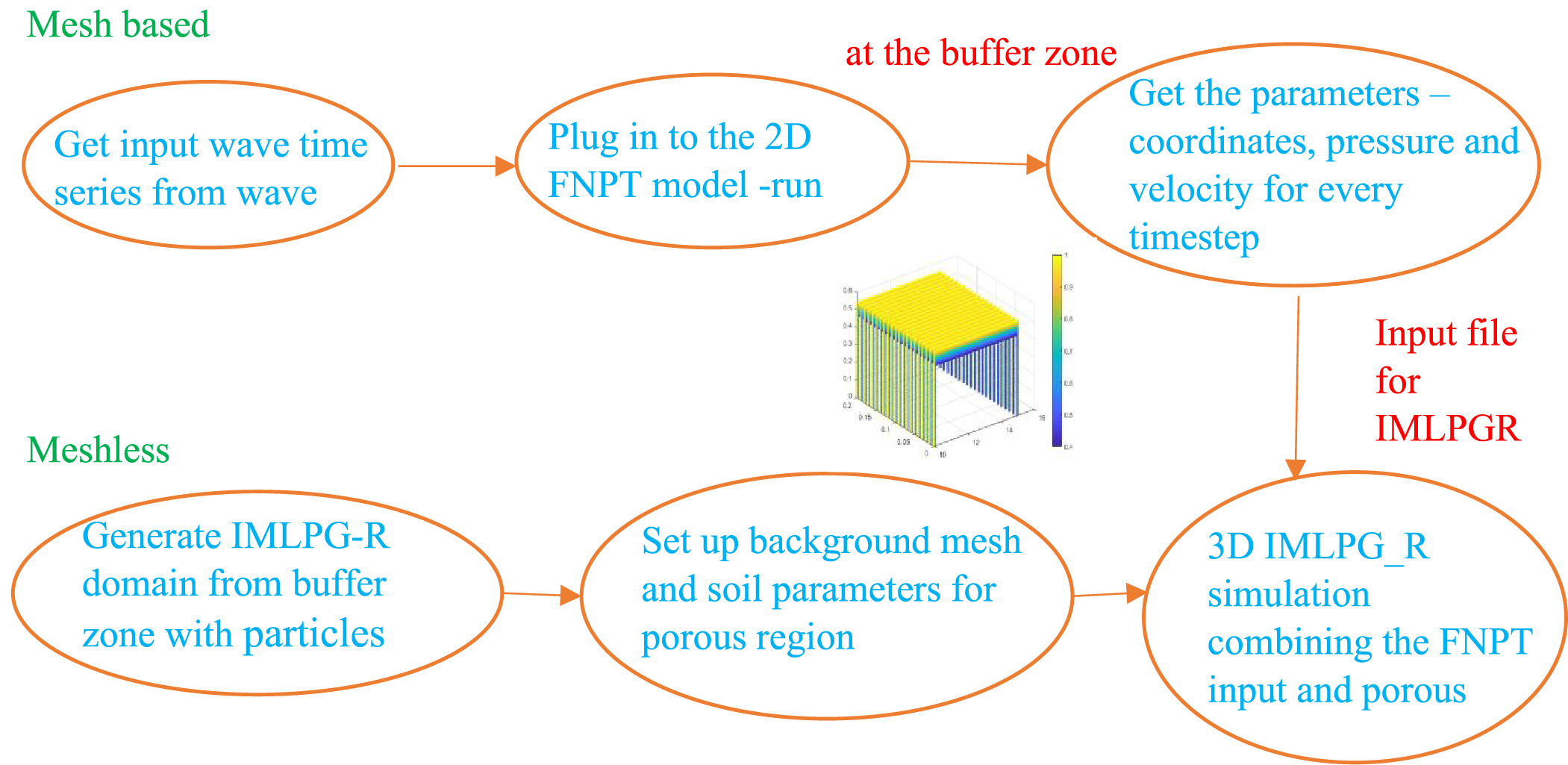
Figure 2: Layout of the hybrid model

3.1 Necessity of PST Algorithm

The existing model is modified to incorporate the sloping bottom. However, during implementation it has been noticed there was a big gap generated at the wall boundaries and the simulation breaks down. The developed algorithm and coefficients are investigated for three cases (a) by including a step (b) by including a steep slope (C) by including a mild slope wall as shown in Fig. 3. The numerical simulation is carried out for each case and investigated for the stability and improvement of accuracy.

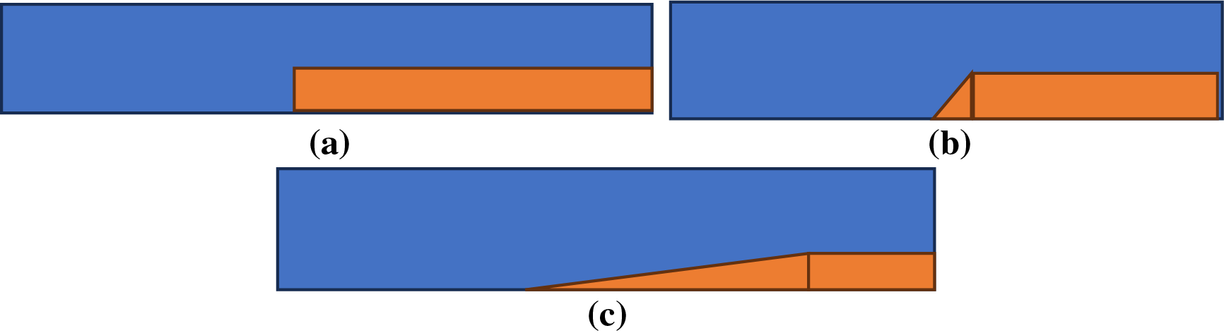
Figure 3: Test cases for different bottom configurations (a) step wall (b) steep slope wall (c) mild slope wall

In order to implement the sloping wall, the following changes are required in the present 3D IMLPG-R model.

a.   Inclusion of Directional components in the computation of Stiffness and Force matrix

b.   Velocity to be updated based on the directional components

These changes are done in the existing 3D IMLPG-R code. Once the changes are carried out, each of the above three cases have been simulated. Ref. [34] gives the details for each sloping bed. The particle arrangement played a significant role in the mild slope wall. When the mild slope wall was arranged with constant number of particles along the water depth as given in Fig. 4a, the simulation stops abruptly. This might be due to two reasons (a) very high particle density above the slope (b) error in the pressure solver is not within the limit. The particle spacing above the slope has been reduced, which further increases the computation time. Thus, the particle arrangements were modified as given in Fig. 4b, where the number of particles along the depth is not constant.

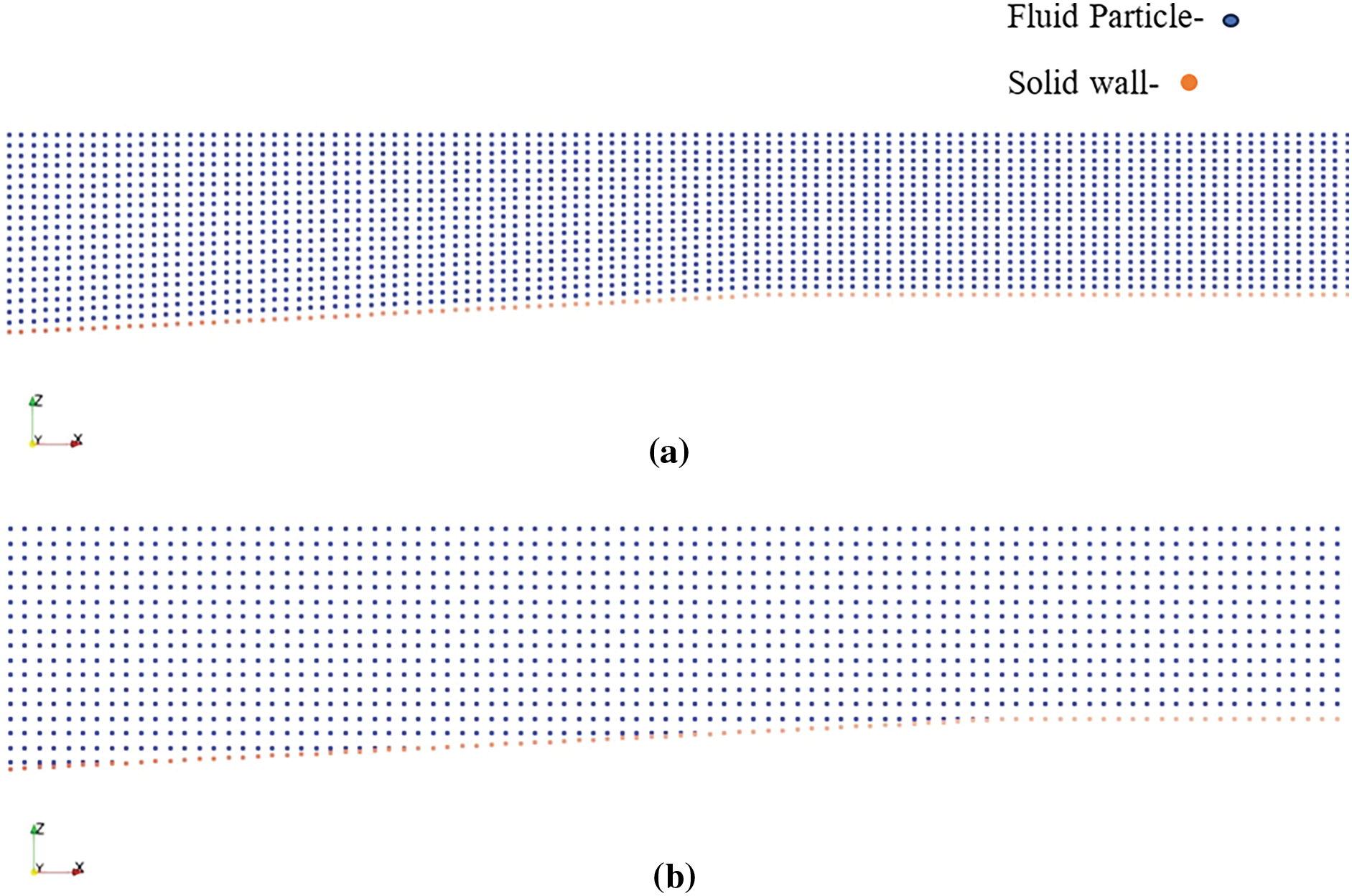
Figure 4: Particle arrangement for mild slope (a) number of particles same across the depth (Arrangement 1) (b) variable number of particles at each x locations across the depth (Arrangement 2)

This arrangement of particle leads to particle gap above the slope as given in Fig. 5. This gap is not prominent on the initial time steps but once a wave passes the slope, it increases. This increase in gap leads to singular matrix meaning there occurs one or more empty rows/columns in the stiffness matrix of the bottom wall particle present below the gap. This would further reduce the accuracy of the simulation in case of regular waves. Thus, particles need to be oriented properly and one needs to avoid the gaps, leading to the implementation of the PST algorithm into the existing 3D IMLPG_R model.

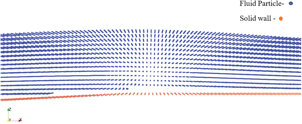
Figure 5: Particle gap between the fluid and bottom wall (x-axis along the length of the tank)

3.2 PST Algorithm

The PST algorithm based on [36] is considered for the present model. PST is based on Fick’s law of diffusion, where the concentration gradient is used. The particles are shifted based on the concentration gradient in each particle. In [36], they have used this PST for incompressible smooth particle hydrodynamic method. The shifting vector δri is computed as given below

δr→i=−h22d⋅∇Ci‖u→‖‖u→max‖(24)

where h is the radius of the influence for particle under consideration, d is the dimension, ∇Ci is the concentration gradient, ‖u→‖ absolute velocity of the particle in consideration, ‖umax‖ is the maximum absolute velocity in the whole domain. The concentration gradient of each particle is computed using the Eq. (25)

∇Ci=∑j[1+Cg⋅(WijW(Δx,h))n]∇iWij(25)

where Wij is the weight function, Ri is the ratio rij/h. The vector rij is the distance between ‘i’ particle and ‘j’ particle. The constants Cg and n are given as 0.2 and 4.0, respectively. Once this shifting vector is arrived for each particle, the velocity and pressure are corrected based on interpolation as below,

ϕinew=∑j=1N∇φj⋅ϕjn+1(26)

where ϕ is the pressure or velocity of the particle under consideration and φj is the shape function of all nearby particle. The weight function Wij and velocity ratio ‖u‖‖umax‖ plays a crucial role in the PST algorithm.

3.3 Optimization of the PST Algorithm

The PST algorithm based on [36] was originally applied for SPH method. Thus, the crucial factors like weight function, the smoothing length, the velocity ratio and the constants are required to be modified for the developed IMLPG-R model. Each parameter has been systematically investigated as given below, so that the particle distribution is well maintained.

3.3.1 Weight Function Optimization

The weight function is a function of the normalized radius or effective radius (r), where the normalized radius is determined by the distance between two nodes. The weight function plays a crucial role in computing the shape functions at each node, as the smoothness of the function depends on the selection of an appropriate weight function in meshless methods. Each weight function exhibits its own behavior in assigning the proper weight to the nodes. Thus, a good weight function will not only provide results that align well with exact solutions, but it should also be robust in terms of convergence and computational efficiency. The following weight functions for the PST were investigated.

Wij=2πh2{316rij2−34rij+34;0≤rij≤20;rij>2(27)

wij={23−4rij2+4rij3;rij≤0.543−4rij+4rij2−163rij3;0.5≤rij≤10;rij>1(28)

Wij=7478πh2×{(2−rij)3−4(1−rij)3,0≤rij<1(2−rij)3,1≤rij<20,rij≥2}(29)

Wij=cπh2{e−rij2;0≤rij≤20;rij>2(30)

Wij={1−6rij2+8rij3−3rij4;rij≤10;rij>1(31)

Wij={e−(rij/0.3);rij≤10;rij>1(32)

where the Eqs. (27)–(29) are the Quadratic spline, Cubic spline, Piecewise quintic, in which Ref. [2] used Piecewise quintic. Eqs. (30)–(32) are Gaussian, Quartic spline and exponential weight function that has been included as it was adopted in our MLPG algorithms. The variation of weight function for normalized radius is given in Fig. 6. It is very clear that the weight values are different for each weight functions and this will impact the PST. To understand, which weight function works efficiently for the developed hybrid model, the Wij value in Eq. (25) is varied based on different weight function given from Eqs. (27)–(32). The simulations are carried out for the numerical stability for each weight function.

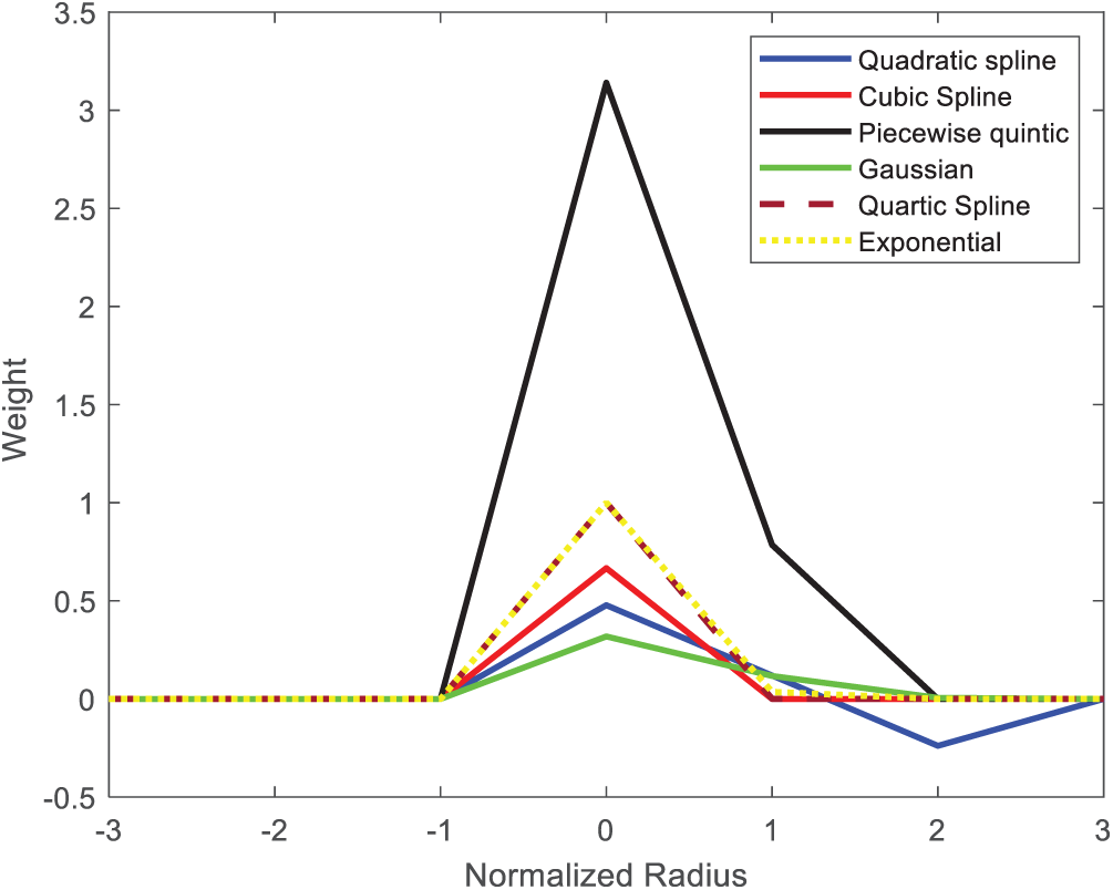
Figure 6: Weight vs. normalized radius for different weight function

Table 1 provides the details of the simulations conducted for each weight function. The total simulation timestep adopted is 3200, with a regular wave height of 0.075 m, a period of 1.6 s, in a water depth of 0.3 m. The numerical tank features a sloping bed that begins at 1 m in the IMLPG_R domain, where the water depth after the slope is set to 0.2 m. The particle spacing adopted is 0.015 m with the timestep of 0.005 s. It was observed that the simulations for the Piecewise, Quartic spline, and Exponential weight functions did not work for the hybrid model. This issue is likely due to the weight exceeding 0.5, when particles are close together, as shown in Fig. 6. Additionally, the weight values for the Quadratic spline, Cubic spline, and Gaussian are below 0.5, meaning that lower weight values would lead to a decrease in concentration gradient, which would further enhance the shifting vector. The issue with the cubic spline and Gaussian functions was their inability to handle the corner near the slope, causing disturbances. Fig. 7 illustrates the errors encountered in these two cases. In the present test case, the distribution from Quadratic spline is better and considered for the further investigation.

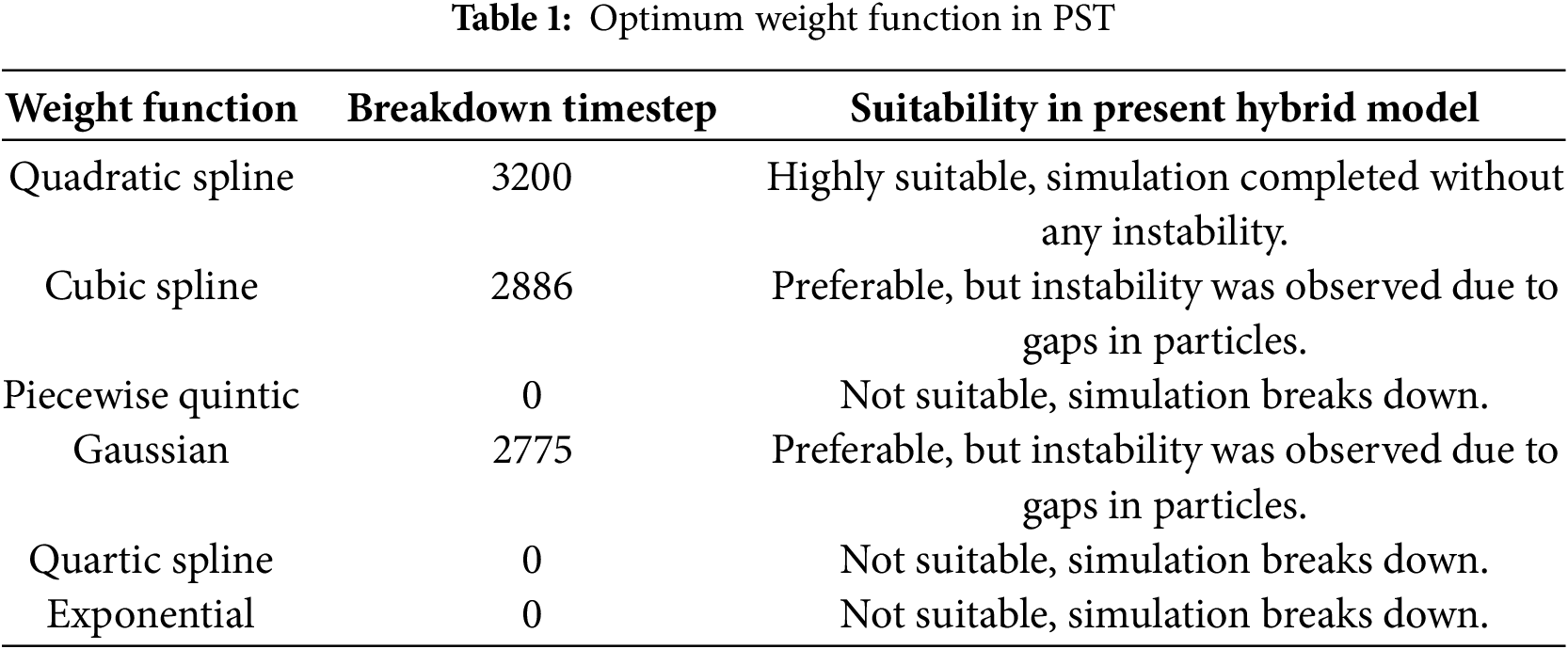
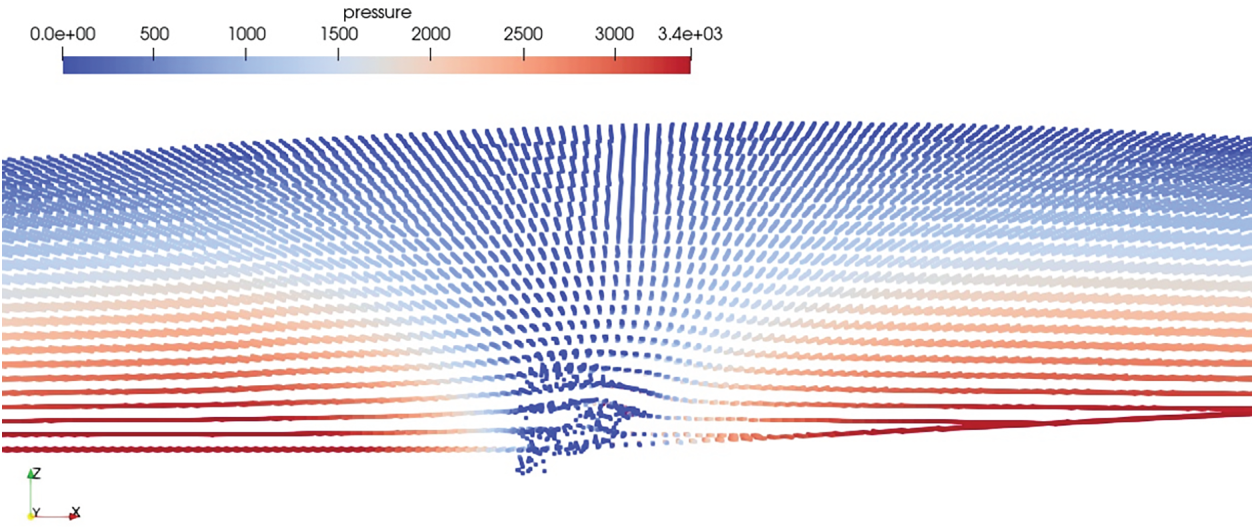
Figure 7: Particle instability using Cubic Spline. Similar observation is noticed for Gaussian Weight and not reproduced (Pressure in Pa). The x-axis along the length of the tank

3.3.2 The Constants and Radius of Influence Domain

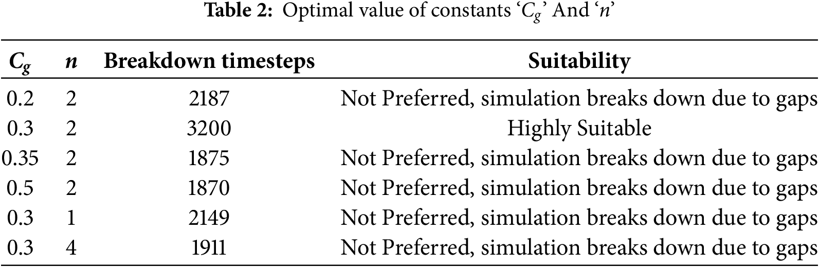
Apart from the weight functions, the other factors like the constants Cg, n in Eq. (25) were investigated and the influence in the results are carried out. Table 2 combines the results for each set of Cg and n values used. It was found that the constant value Cg = 0.3 and n = 2 is found to be suitable.

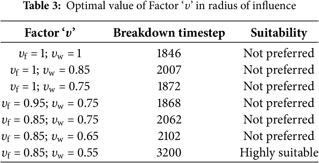
The next factor which was taken into consideration was the radius of influence ‘h’. The ‘h’ value was taken as an average of the hi and hj in a domain. This means when weight of particle ‘i’ is computed then the hij = υ* (hi +hj)/2 is used, in which hi is the radius of influence of ‘i’ particle and hj is the radius of influence of ‘j’ particle. This was considered to take into the effect of the j particle. A factor ‘υ’ is multiplied to this average value to get the optimum value, this works better for the developed model. Table 3 gives the details of the factor ‘υ’ that works better for the PST algorithm. It was also found that same value of ‘υ’ didn’t work out well for fluid and wall particles, hence different values are adopted. It was found that for factor υf = 0.85 and υw = 0.55, there was no numerical instability occurred and this value is considered for further studies.

3.3.3 Velocity Ratio on the Boundary

The final factor which plays a crucial role in PST algorithm is the velocity ratio in Eq. (24). To verify the effect of this ratio, a solitary wave case in the same numerical tank has been considered, as it is a translatory waves and velocities will be higher. Here, all the three-direction velocity (u, v, w) are considered in shifting the particle in three different directions (x, y, z). The ratio of velocity ‖u‖‖umax‖ is taken in all three directions and verified for different values and final optimal value has been arrived. The application of this ratio has to be carried out carefully on the moving boundary, where the input from FNPT is taken, since the ratio will be higher for these boundaries leading to higher shifting vector for the particles near the moving boundary. Fig. 8 shows the gap obtained due to higher shifting of the particles in ‘x’ direction as the ‖u‖‖umax‖ is more than 1 in x direction alone. It is to be noted in the figure that the left-hand side corner is the moving boundary which takes the input from FNPT. To avoid this, the PST algorithm is applied on the buffer zone region gradually by introducing an exponential term.

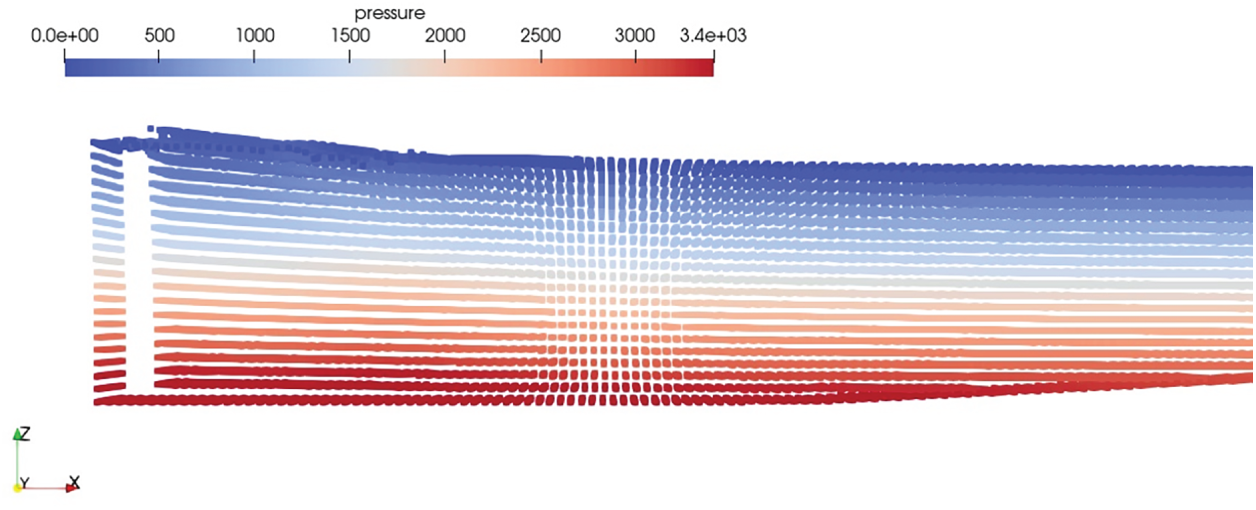
Figure 8: Effect of high shifting vector in x direction on the moving boundary (The colormap represents the pressure in Pa)

Similar scenario happens in the case of the free surface particles, when the shifting vector is applied to free surface and the particles near the free surface try to get out of the domain. To avoid this, shifting vector is gradually introduced from free surface also. Fig. 9 shows the effect of higher shifting of fluid particles near the free surface. To avoid this, the shifting vector would be zero at the free surface and linearly increases as the particles distant away from free surface. Further the velocity ratio on the y direction, which is along the width of the domain, is also restricted as the particle shifting along this direction lead to higher clustering. Fig. 10 shows the clustering of particles when the z direction velocity ratio is not restricted and Fig. 11 shows the improvement in the particle distribution when the shifting in z direction is restricted.

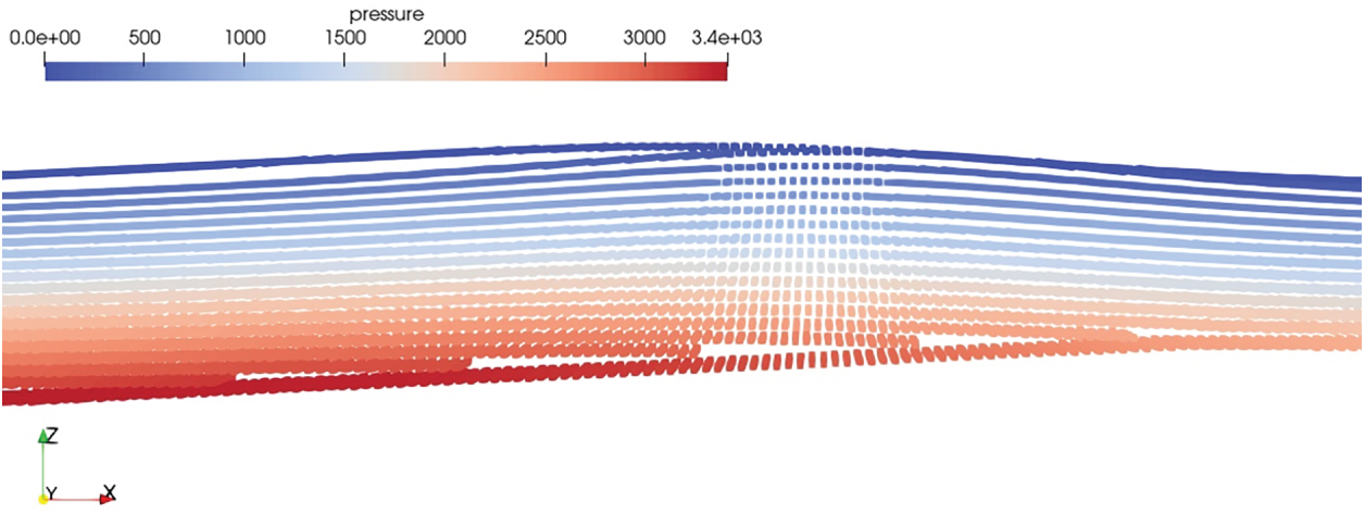
Figure 9: Effect of high shifting of fluid particles towards free surface (The colormap represents the pressure in Pa)

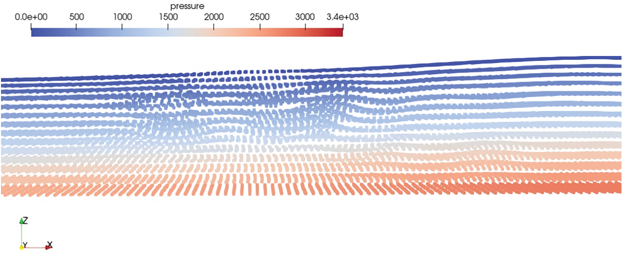
Figure 10: Clustering of Particles in ‘z’ Direction (The colormap represents the pressure in Pa)

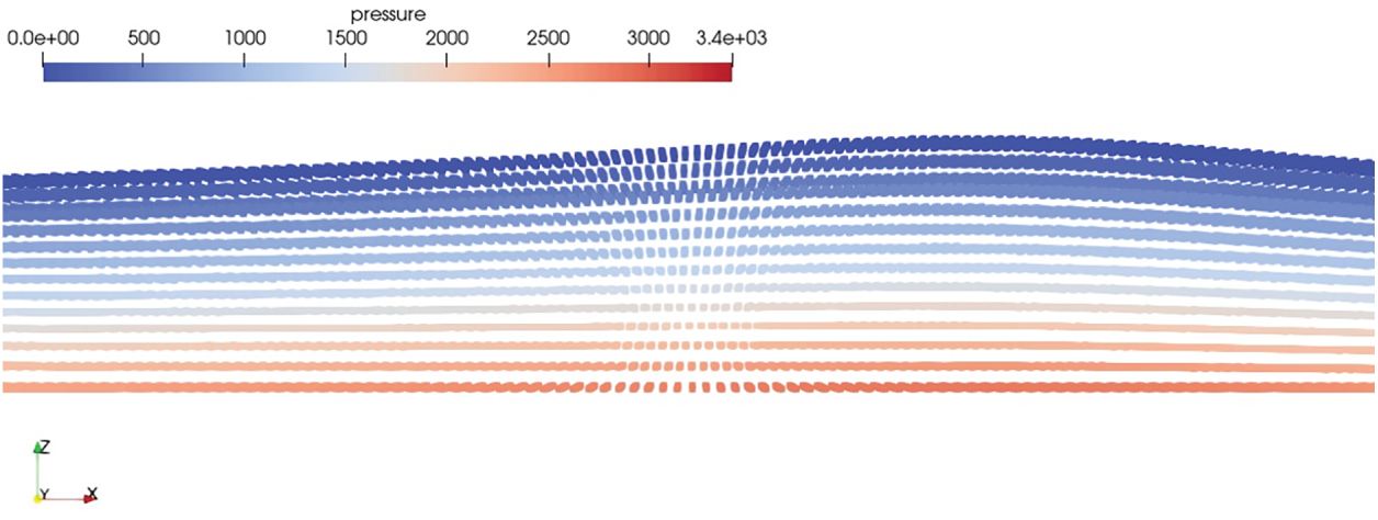
Figure 11: Clustering avoided with restriction in ‘z’ with velocity ratio constraints (The colormap represents the pressure in Pa)

The velocity ratio as per [36] was reported as 0.2 h/Δt which didn’t work out for our cases; hence the ratio was fixed based on trial and error and we have modified based on the maximum velocity limit as given below

‖u‖‖umax‖≤0.05umax(33)

Once the algorithm is incorporated into the model, the solitary wave has been simulated again without any influence of the porous layer to verify whether the particle distribution is enhanced and investigate for any numerical instability. Fig. 12 shows the solitary wave passed above the mild slope with PST algorithm. It is evident from the Fig. 12 that the particle distribution is enhanced by moving the particle from high concentration region of the slope to low concentration region of bottom wall above slope and no numerical instability was observed.

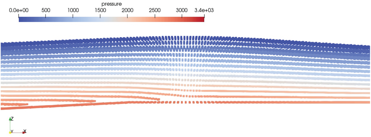
Figure 12: Solitary wave with PST algorithm (The colormap represents the pressure in Pa)

3.4 Interpolation in Background Mesh

Similar to our previous study in [30], stationary background (BG) nodes are used for the implementation of the porosity. A smooth transition of the porous rate value is provided in the BG nodes. These BG nodes are used by the IMLPG_R particles to interpolate the porous rate value of each particle in the interface layer. Simplified finite difference interpolation (SFDI) by [51] is used for the porosity interpolation of the particles. For a fluid particle in the interface region, a sphere consisting of the BG nodes is taken into consideration for interpolation. The sphere has a radius of three times the BG node distance. Each fluid particle is connected to maximum of 32 BG nodes. This is to reduce the computation time. Fig. 13 gives the schematic representation of the BG nodes (open circle) connection to a fluid particle (closed circle). It was observed that in our 2D case, the BG node transition was applied for twice the initial particle distance. However, for our developed 3D model such an extended transition region was not required. The reason may be due to the fact that the interpolation occurred in three dimensions, the velocity transitioned smoothly from the pure fluid to the pure porous region, with minimal to no transition zone.

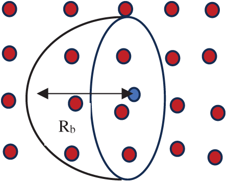
Figure 13: Schematic representation of BG nodes and fluid particle connection

3.5 Critical Parameters in 3D Porous Model

The developed porous model was validated against cases involving emerged porous structures unlike the previous study in 2D which focused solely on submerged structures. For a submerged porous structure implementation, the velocity components are lower and the transition in velocity from the fluid region to the porous region is relatively smooth whereas in an emerged type of porous structure, the fluid velocity is higher and so the gradient is higher from fluid region to porous region. According to Eq. (15), both fluid and Darcian velocities are significantly influenced by the porosity. When porosity is low and Darcian velocity is high, a steep velocity gradient forms between the fluid and porous regions. This sharp gradient led to issues with particle distribution in the simulation. To avoid this and to maintain a smoothness in the particle distribution, three minor changes are implemented in the developed model.

(1)   Maintaining the same velocity component in the Force matrix during numerical integration

(2)   Smooth the porosity value using SFDI method at the interface after the porosity value has been arrived based on background mesh and the drag constants.

(3)   Update the particle position based on the Darcian velocity and not based on Fluid velocity.

3.5.1 Velocity Components in Force Matrix

The final, simplified formulation relating the stiffness matrix to the force matrix, with the left-hand side incorporating velocity components along all six points, is given in Eq. (23). At the fluid–porous interface, assigning Darcy velocity components directly to interface particles in emerged configurations introduces significant discontinuities due to the pronounced velocity mismatch. This loss of velocity field continuity can compromise numerical stability and accuracy. To mitigate such discrepancies, key parameters such as porosity and inertial resistance coefficients are incorporated on a per-particle basis during numerical integration, rather than being applied solely at the evaluation point. This approach ensures more accurate representation of interfacial dynamics and enhances computational robustness. Thus, Eq. (23) becomes,

16(p1+p2+p3+p4+p5+p6)−p0=ρwdt∗RI12(cr∗uD1∗nw−cr∗uD3∗nw+cr∗vD2∗nw−cr∗vD4∗nw+cr∗wD5∗nw−cr∗wD6∗nw)(34)

This ensures that the velocity is smooth throughout the considered numerical points and not specific to the point under consideration. This is required, since the porous structure are normally having a trapezoidal shape, such as breakwaters.

3.5.2 Porosity Smoothing and Drag Constants

The porosity is updated at every time step using the background mesh. To smoothly transfer the porosities at the interface, interpolation using SFDI is carried out. To interpolate the porosity of particle ‘i’, the nearby ‘j’ particle’s porosity has been used. The ‘j’ particles are linked to ‘i’ throughout the interpolation, which means to calculate the force matrix, stiffness matrix and for the pressure gradient these ‘j’ particles are only used. So, interpolating the porosities of ‘i’ using this ‘j’ particle’s porosity increases the accuracy of the developed model and no discontinuity is present in the porosities. Eq. (35) shows the interpolation used for the porosity value at each time step where the φj is the shape function based on SFDI.

nwinew=∑j=1Nφj⋅nwjn+1(35)

The next important parameter deciding the accuracy of the simulation was the drag constants used in the linear and non-linear drag forces as given in Eqs. (8) and (9). Since the developed model is based on unified governing equations, the additional drag forces were zero for the case of pure fluid and non-zero in the porous region. These additional forces further depended on the Darcian velocity. Thus, in case of emerged porous region when a Darcian velocity was higher and the drag constants ‘a’ and ‘b’ were higher, leading to occurrence of a huge gradient of velocity. When a constant porosity value is used as given in Eq. (9), the velocity varies from positive to negative as given in Fig. 14. The velocity outside the porous region was higher and the velocity inside was drastically reduced. This led to fluid region particle to move faster than that of the porous region particle. Fig. 15a shows the variation of the linear drag force constants with porosity. To avoid this discontinuity, the additional drag force constants were also modified based on the particle porosity. Hence, Eq. (9) was changed to Eq. (36), where nwi is the porosity of the particle under consideration and nw is the constant porosity value which means the constants ‘a’ and ‘b’ will be varying along with the porosity values. The continuity is maintained in this modification and the reduction of the velocity is also smooth from pure fluid to pure porous region. The values k = 2, m = 3, n = 2, α = 1000 and β = 1.1 for this test case,

a=αϑw(1−nwi)2nwi3D502b=β1−nwinwi3D50Cr=1+1−nwinwiγ with γ=0.34(36)

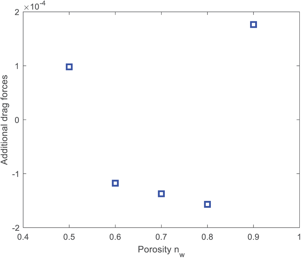
Figure 14: Variation of velocity for a constant porosity value in different region

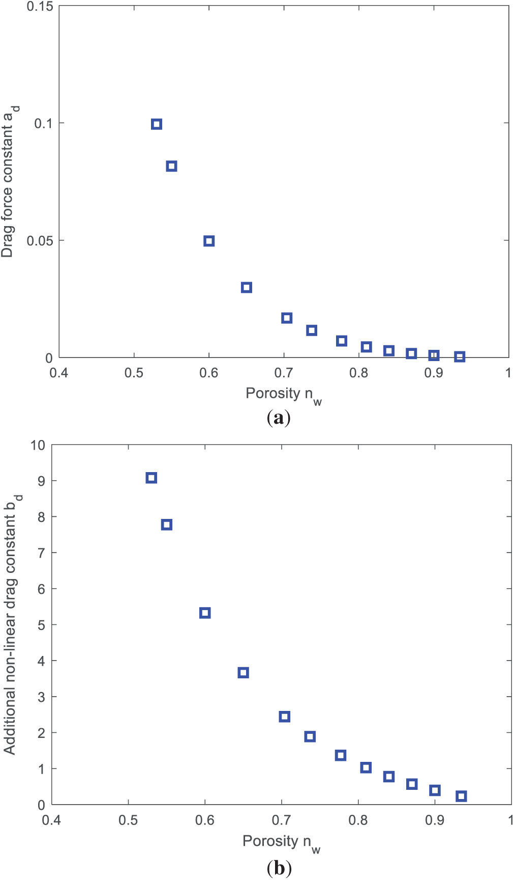
Figure 15: Variation of (a) linear ‘a’ (b) non-linear ‘b’ drag force constants with respect to different porosity value

3.5.3 Updating the Particle Position Based on Darcian Velocity

The other issue encountered during the emerged porous model was the high particle movement in the porous region than that of the pure fluid region. The study done in [52] gives the detailed explanation of this issue. The particle position updated based on the fluid velocity as given in Eq. (16) led to the higher movement of particle inside the porous region, since the fluid velocity is divided by the porosity value as given in Eq. (15). When the Darcian velocity is higher in case of emerged, porous structure dividing the porosity value further increases the fluid velocity inside the porous region there by the particle movement is also higher in the porous region. In the previous study, since the porous structure was submerged, the Darcian velocity and fluid velocity difference was meagre due to which Eq. (16) worked out fine. In the pure fluid region, both fluid velocity and the Darcian velocity is the same. Hence the Eq. (16) is now changed to Eq. (37) as given below,

x→n+1=x→n+u→Dn+1dt(37a)

y→n+1=y→n+v→Dn+1dt(37b)

z→n+1=z→n+w→Dn+1dt(37c)

4  Validation of the Numerical Model

Once the model is developed with PST algorithm, validation for wave porous structure interaction is carried out for which a single layer trapezoidal porous layer in a flat bottom bed has been considered. Then a second case of both porous sloping bed and impermeable sloping bed is simulated which is compared with experimental and numerical results.

4.1 Trapezoidal Porous Layer

The experimental results from [53] is considered. The numerical tank with a total length of 14 m is considered in which first 4 m is simulated using FNPT model and the remaining is simulated in 3D IMLPG_R with a water depth of 0.376 m and width 0.376 m. The incoming uni-directional regular wave height of 0.092 m and wave period of 1.6 s was considered for the simulation. The trapezoidal porous layer has a height of 0.33 m with front slope of 1H:2V and starts at 1.5 m from the beginning of IMLPG_R model. The buffer zone of 0.5 m is provided and the wave damping zone of 3 m is considered at the far end of the domain. The buffer zone length was determined based on the numerical experiments carried out by [43]. The trapezoidal porous layer has a porosity value of 0.45 (nw) with the soil particle size of 0.025 m (D50) having α, β, m, n as 1000, 1.1, 3 and 2, respectively. The inertia coefficient Cr is assumed as 1. The wave height is compared at different wave gauge position at 4.03, 5.33, 5.83, 6.68 and 7.37 m. The computational setup is as given in Fig. 16. The wave profile on the wave gauges is compared and the results are given in Fig. 17. The comparison is reasonable. The absolute error between the experimental values and the values from 3D IMLPG_R is calculated for the wave gauge reading at 7.37 m and is presented in the Fig. 18. The absolute error is computed as the absolute difference between the experimental data and the corresponding results obtained from the 3D IMLPG-R method and is given by |ηexp−ηIMPLG_R|.

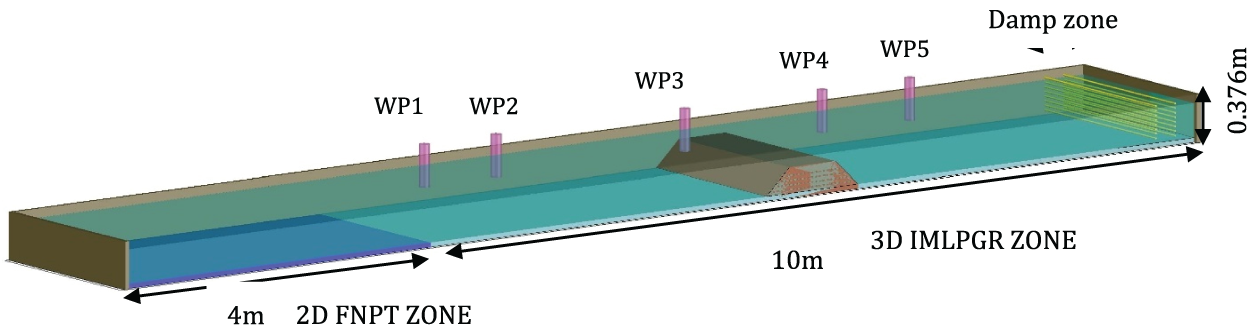
Figure 16: Computational domain for single porous layer based on [53]

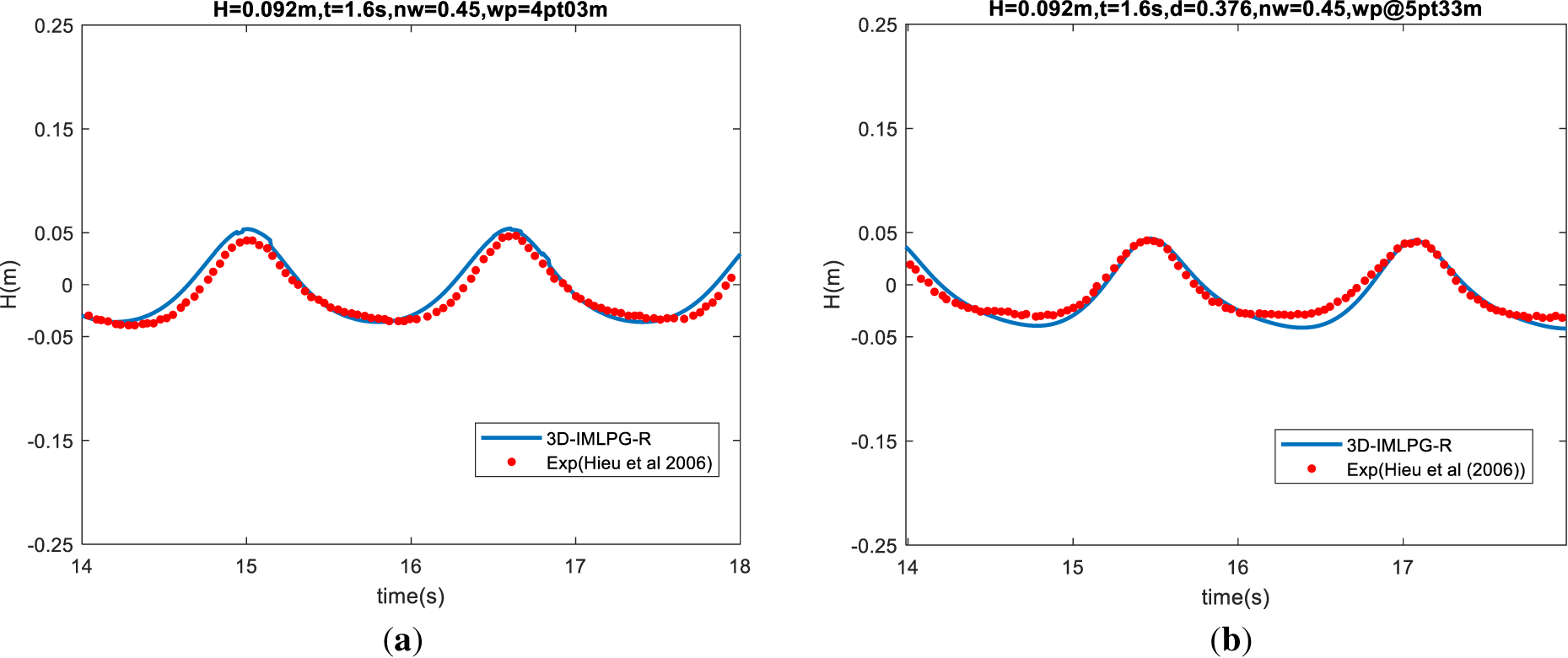
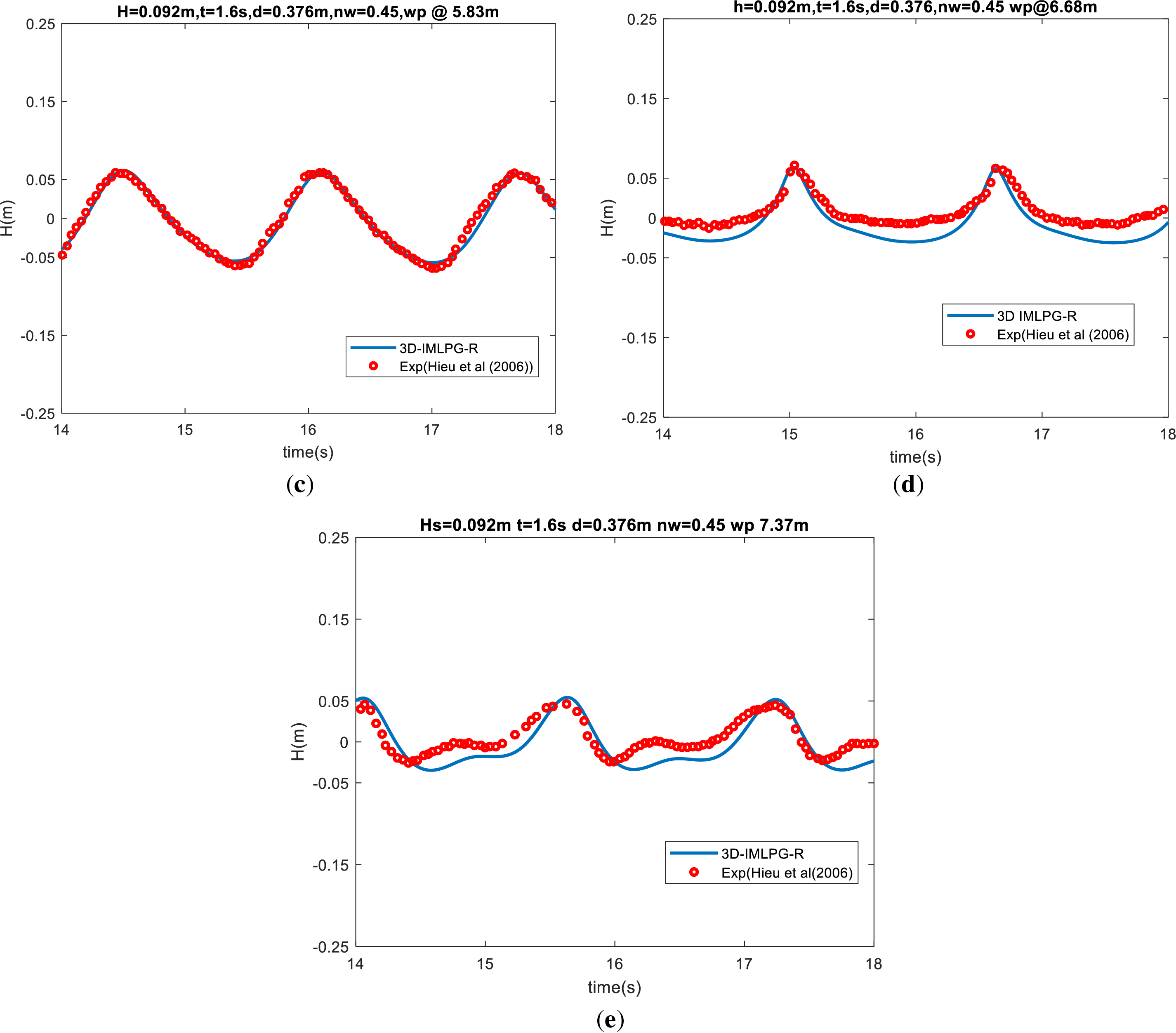
Figure 17: Comparison of hybrid model results with experimental results of [53] at (a) WP1 = 4.03 m (b) WP2 = 5.33 m (c) WP3 = 5.83 m (d) WP4 = 6.68 m (e) WP5 = 7.37 m

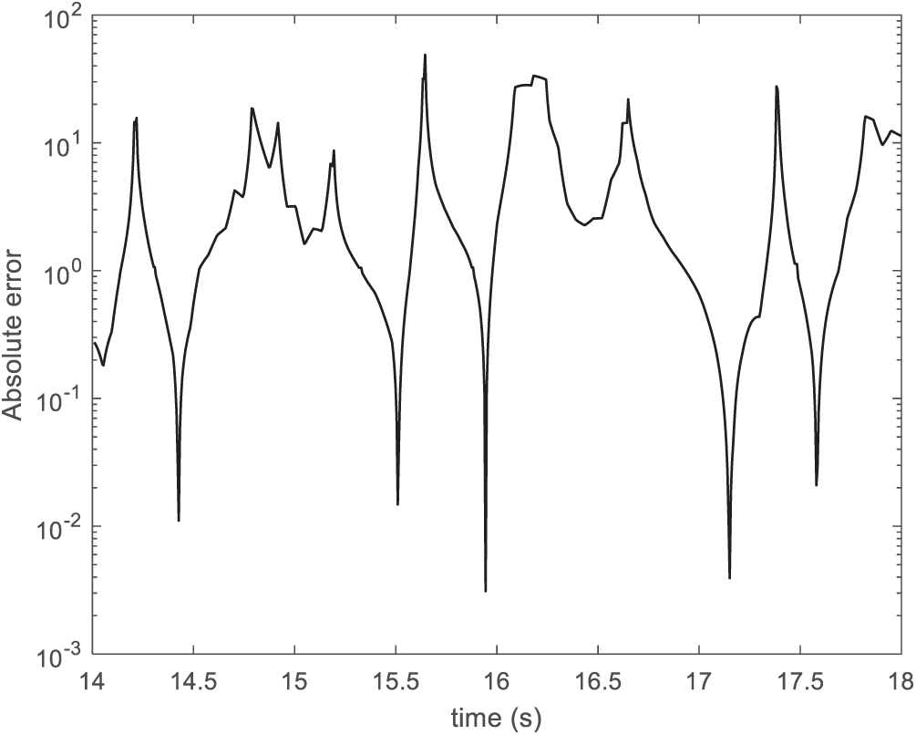
Figure 18: Absolute error at WG5 (7.37 m) between [53] and 3D IMLPG-R

Fig. 19 shows the initial set up of the numerical tank in 3D IMLPG-R domain with the trapezoidal porous structure present. Fig. 20 shows the isometric view of the 3D IMLPG_R numerical tank as the wave propagates. Fig. 21a shows the wave trough passing over the porous structure and Fig. 21b shows the wave crest passing over the trapezoidal structure. It is evident from the picture that the wave profile is affected by the porous structure. Fig. 22 shows the velocity components when a wave passes over the trapezoidal structure.

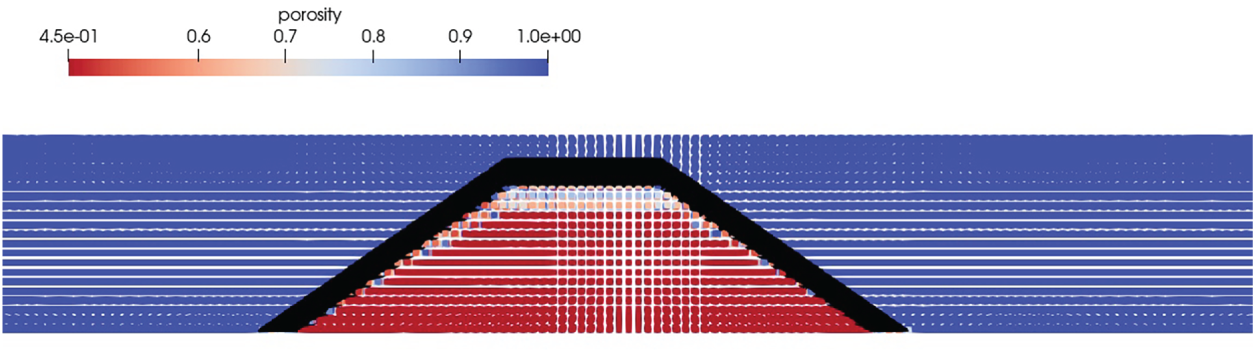
Figure 19: Initial setup of the Numerical wave tank with the cross-sectional view along the length of the tank (The colormap represents the porosity)

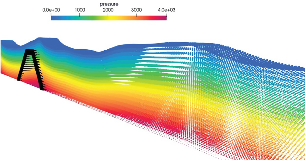
Figure 20: Wave propagation in the isometric view (The colormap represents the pressure in Pa along the length of the tank)

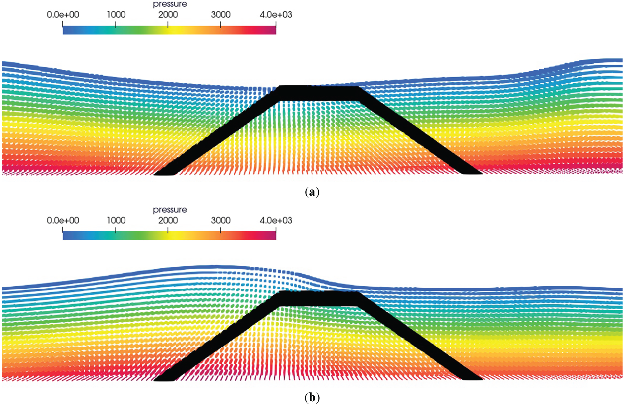
Figure 21: Screenshot of (a) trough over the porous structure (b) Crest over the porous structure (The colormap represents the pressure in Pa along the length of the tank)

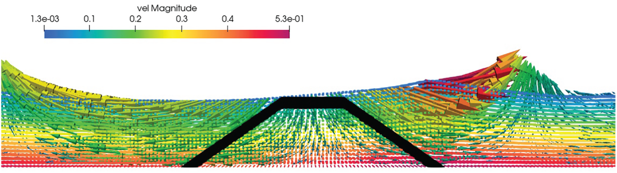
Figure 22: Velocity vectors during wave propagation (The colormap represents the velocity in m/s along the length of the tank)

4.2 Porous Sloping Bed and Impermeable Sloping Bed

The experimental results from [54] is used where the sloping bed is considered to be porous. Numerical tank is divided into two where the first 5 m is simulated in 2D FNPT model and remaining 7 m is simulated in 3D IMLPG_R model with a buffer zone of length 0.5 m starting at 5 m. The slope starts at 2 m in 3D IMLPG_R domain and ends at 2.762 m with a slope of 1:20. Water depth is taken as 0.0762 m before slope and 0.0381 m after slope. Two simulations are done, one with impermeable sloping bed and another with porous sloping bed with a porosity value of 0.3. The solitary wave height of 0.009 m is simulated and wave height at 1.593, 3.651 and 4.5146 m in IMLPG_R domain is compared. Fig. 23a illustrates the porous sloping bed and Fig. 23b shows the impermeable sloping bed. The wave profile is compared for both porous and impermeable sloping bed. Fig. 24 shows the compared wave profile at different location. It is evident that more than the impermeable sloping bed the porous bed gave better solution. The 3D IMLPG_R model performs well with porous bed and the solution is better than that of the numerical simulation of [55] which has used Weakly Compressible Smooth Particle Hydrodynamics (WCSPH) to solve this test case. The study does not account for turbulence effects. Nevertheless, as shown in Fig. 24, the current model demonstrates improved accuracy, with the velocity exhibiting a smooth transition across the interface zone despite the exclusion of turbulence The model developed was an impermeable mild slope wall. Fig. 25 presents the absolute error at the wave gauge located at 4.5146 m, computed between the experimental and simulated results, consistent with the approach used in the previous section.

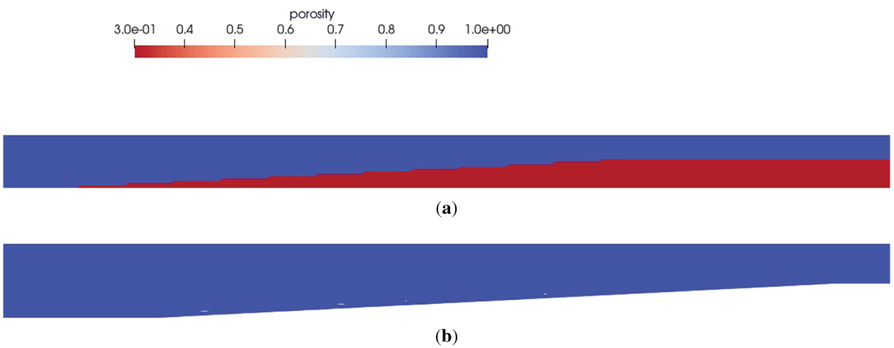
Figure 23: Initial set up of the numerical tank (a) with porous bed (b) without porous bed (The colormap represents the porosity)

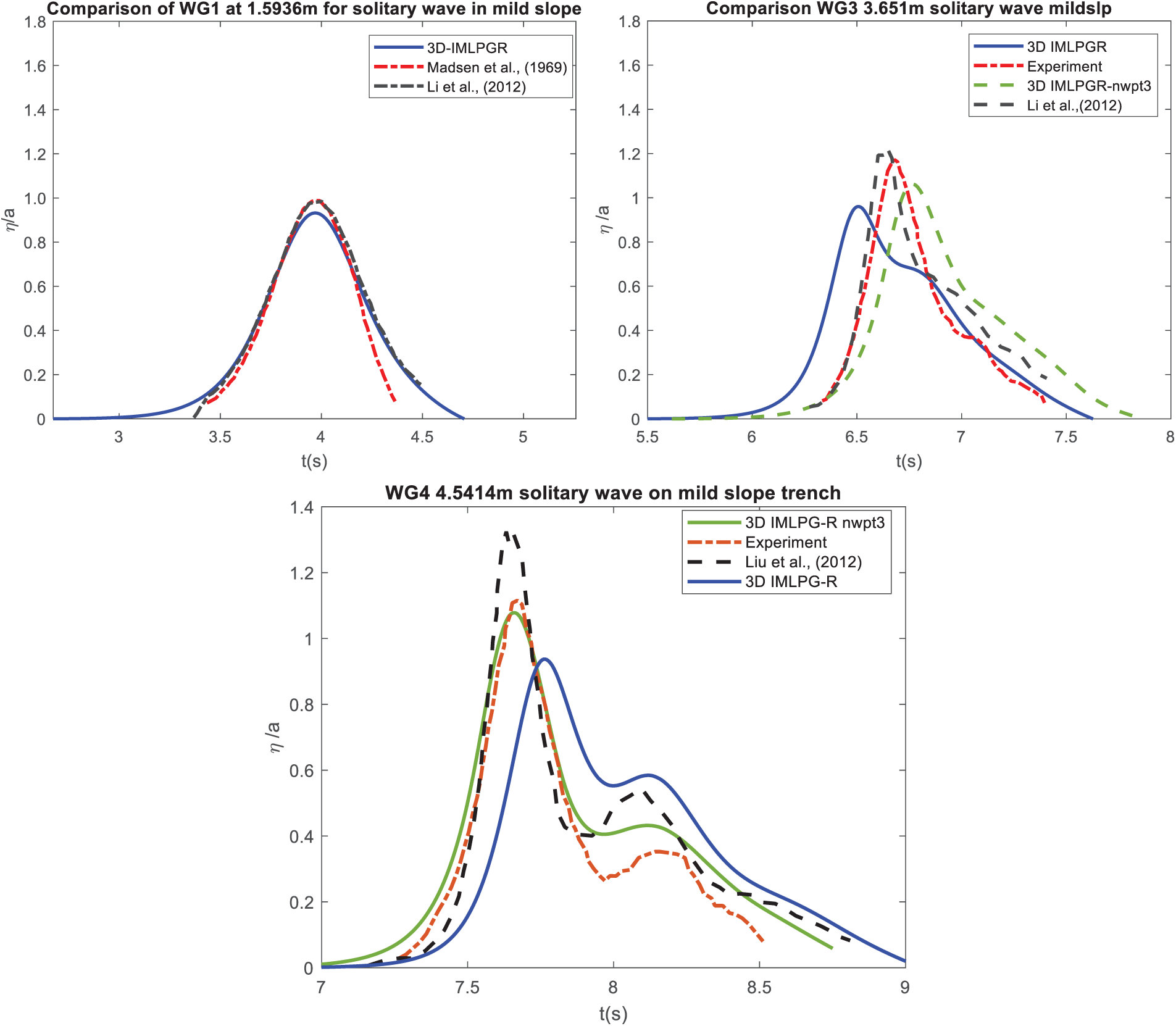
Figure 24: Wave profile at different location for porous bed of nw 0.3 (Green) and impermeable bed (Blue) compared with experimental results from [54] and numerical results from [55]

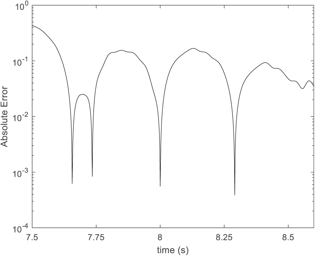
Figure 25: Absolute error at WG (4.5146 m) between the experiments and 3D IMLPG-R

5  Conclusion

This study presents a three-dimensional model developed to simulate wave interaction with porous structures. The approach weakly couples a two-dimensional Fully Nonlinear Potential Theory (FNPT) model with a three-dimensional Improved Moving Least Squares-based Point Galerkin (IMLPG-R) model where the turbulence effect is not considered. The developed model incorporates a smooth porosity transition across the interface, effectively reducing sharp velocity gradients in this region. This treatment suppresses the formation of localized turbulent jets and ensures consistency with the laminar flow assumption adopted in the present study. Previous SPH models for porous flow encountered two major challenges: (i) pressure or velocity fluctuations at the interface, and (ii) the need for iterative evaluation of porosity values at each time step. The present model addresses both issues. Within the IMLPG-R framework, the absence of a pressure gradient term in the stiffness matrix mitigates interface fluctuations, while the SFDI method provides porosity values at each time step directly, eliminating the need for iteration

The paper provides a detailed account of the mathematical formulation and the numerical algorithm employed. The primary focus is on the 3D IMLPG-R implementation, specifically its application to porous structures. While previous implementations of the 3D IMLPG-R model considered flat beds, this study extends it to include sloping beds. Incorporating the slope introduced several issues related to particle distribution in our 3D model, which were addressed using a Particle Shifting Technique (PST) based on the method proposed by [36]. The PST algorithm was optimized to best fit the developed model by fine-tuning several parameters such as the weight function, velocity ratio, constants, and radius of influence through a trial-and-error process. The importance of these parameters is investigated thoroughly in the present study.

The paper also describes the implementation of the numerical algorithm on a 3D background mesh and highlights challenges encountered when introducing an emerged trapezoidal porous structure. Three major challenges are discussed: maintaining uniformity in the force matrix, consistency in porosity and drag coefficient values, and accurate updating of the particle positions.

Furthermore, this study presents the modifications implemented in the three-dimensional (3D) numerical algorithm, extending the framework developed in the previous two-dimensional (2D) study. The model’s accuracy is verified through simulations of regular wave interactions with a single trapezoidal porous structure. Subsequent validations are performed for both porous and impermeable bed conditions, demonstrating good agreement with experimental results. It is noteworthy that the present investigation is limited to laminar flow, as the governing equations do not incorporate turbulence effects. The developed PST algorithm is further applied to a sloping bed configuration, where the earlier particle redistribution approach proved ineffective.

Acknowledgement: The first author gratefully acknowledges the financial support received from the Prime Minister’s Research Fellowship (PMRF), which facilitated the completion of this work.

Funding Statement: This research was funded by Prime Minister’s Research Fellowship (PMRF), grant number SB22230924OEPMRF008608.

Author Contributions: The authors confirm the contribution to the paper as follows: Conceptualization, Divya Ramesh and Sriram Venkatachalam; methodology, Sriram Venkatachalam and Divya Ramesh; coding, Divya Ramesh; validation, Divya Ramesh; investigation, Divya Ramesh; writing—original draft preparation, Divya Ramesh; writing—review and editing, Sriram Venkatachalam; supervision, Sriram Venkatachalam. All authors reviewed the results and approved the final version of the manuscript.

Availability of Data and Materials: The authors confirm that the data supporting the findings of this study are available within the article.

Ethics Approval: Not applicable.

Conflicts of Interest: The authors declare no conflicts of interest to report regarding the present study.

References

1. McCorquodale JA. Wave dissipation in rockfill. In: Proceedings of 13th Coastal Engineering Conference. New York, NY, USA: ASCE; 1972. p. 1885–900. [Google Scholar]

2. Lin P, Liu PL. A numerical study of breaking waves in the surf zone. J Fluid Mech. 1998;359:239–64. doi:10.1017/s002211209700846x. [Google Scholar] [CrossRef]

3. Huang CJ, Shen ML, Chang HH. Propagation of a solitary wave over rigid porous beds. Ocean Eng. 2008;35(11–12):1194–202. doi:10.1016/j.oceaneng.2008.04.003. [Google Scholar] [CrossRef]

4. Karim MF, Tanimoto K, Hieu PD. Modelling and simulation of wave transformation in porous structures using VOF based two-phase flow model. Appl Math Model. 2009;33(1):343–60. doi:10.1016/j.apm.2007.11.016. [Google Scholar] [CrossRef]

5. Liu PL, Lin P, Chang KA, Sakakiyama T. Numerical modeling of wave interaction with porous structures. J Waterw Port Coast Ocean Eng. 1999;125(6):322–30. doi:10.1061/(asce)0733-950x(1999)125:6(322). [Google Scholar] [CrossRef]

6. Losada IJ, Lara JL, Guanche R, Gonzalez-Ondina JM. Numerical analysis of wave overtopping of rubble mound breakwaters. Coast Eng. 2008;55(1):47–62. doi:10.1016/j.coastaleng.2007.06.003. [Google Scholar] [CrossRef]

7. Stahlmann A, Schlurmann T. Investigations on scour development at tripod foundations for offshore wind turbines: modeling and application. Int Conf Coastal Eng. 2012;(33):90. doi:10.9753/icce.v33.sediment.90. [Google Scholar] [CrossRef]

8. Hu KC, Hsiao SC, Hwung HH, Wu TR. Three-dimensional numerical modeling of the interaction of dam-break waves and porous media. Adv Water Resour. 2012;47:14–30. doi:10.1016/j.advwatres.2012.06.007. [Google Scholar] [CrossRef]

9. del Jesus M, Lara JL, Losada IJ. Three-dimensional interaction of waves and porous coastal structures. Coast Eng. 2012;64:57–72. doi:10.1016/j.coastaleng.2012.01.008. [Google Scholar] [CrossRef]

10. Higuera P, Lara JL, Losada IJ. Three-dimensional interaction of waves and porous coastal structures using OpenFOAM®. Part II: application. Coast Eng. 2014;83:259–70. doi:10.1016/j.coastaleng.2013.09.002. [Google Scholar] [CrossRef]

11. Ren B, Wen H, Dong P, Wang Y. Improved SPH simulation of wave motions and turbulent flows through porous media. Coast Eng. 2016;107:14–27. doi:10.1016/j.coastaleng.2015.10.004. [Google Scholar] [CrossRef]

12. Wen H, Ren B, Dong P, Zhu G. Numerical analysis of wave-induced current within the inhomogeneous coral reef using a refined SPH model. Coast Eng. 2020;156:103616. doi:10.1016/j.coastaleng.2019.103616. [Google Scholar] [CrossRef]

13. Basser H, Rudman M, Daly E. Smoothed particle hydrodynamics modelling of fresh and salt water dynamics in porous media. J Hydrol. 2019;576:370–80. doi:10.1016/j.jhydrol.2019.06.048. [Google Scholar] [CrossRef]

14. Kazemi E, Tait S, Shao S. SPH-based numerical treatment of the interfacial interaction of flow with porous media. Int J Numer Methods Fluids. 2020;92(4):219–45. doi:10.1002/fld.4781. [Google Scholar] [CrossRef]

15. Kazemi E, Luo M. A comparative study on the accuracy and conservation properties of the SPH method for fluid flow interaction with porous media. Adv Water Resour. 2022;165(1):104220. doi:10.1016/j.advwatres.2022.104220. [Google Scholar] [CrossRef]

16. Su X, Wang C, Luo M, Zhan Y. Development of a smoothed particle hydrodynamics model for porous media flows with enhanced volume conservation and the revisit of the mass conservation equation. Phys Fluids. 2024;36(10):103116. doi:10.1063/5.0231042. [Google Scholar] [CrossRef]

17. Kazemi E, Koll K, Tait S, Shao S. SPH modelling of turbulent open channel flow over and within natural gravel beds with rough interfacial boundaries. Adv Water Resour. 2020;140(1):103557. doi:10.1016/j.advwatres.2020.103557. [Google Scholar] [CrossRef]

18. Akbari H, Torabbeigi M. SPH modeling of wave interaction with reshaped and non-reshaped berm breakwaters with permeable layers. Appl Ocean Res. 2021;112(1):102714. doi:10.1016/j.apor.2021.102714. [Google Scholar] [CrossRef]

19. Tsurudome C, Liang D, Shimizu Y, Khayyer A, Gotoh H. Study of beach permeability’s influence on solitary wave runup with ISPH method. Appl Ocean Res. 2021;117(1):102957. doi:10.1016/j.apor.2021.102957. [Google Scholar] [CrossRef]

20. Awad BN, Tait MJ. Macroscopic modelling for screens inside a tuned liquid damper using incompressible smoothed particle hydrodynamics. Ocean Eng. 2022;263:112320. doi:10.1016/j.oceaneng.2022.112320. [Google Scholar] [CrossRef]

21. Chen YK, Meringolo DD, Liu Y, Liang JM. Energy balance during Bragg wave resonance by submerged porous breakwaters through a mixture theory-based δ-LES-SPH model. Coast Eng. 2025;196(1):104652. doi:10.1016/j.coastaleng.2024.104652. [Google Scholar] [CrossRef]

22. Ding D, Ouahsine A, Xiao W, Du P. CFD/DEM coupled approach for the stability of caisson-type breakwater subjected to violent wave impact. Ocean Eng. 2021;223:108651. doi:10.1016/j.oceaneng.2021.108651. [Google Scholar] [CrossRef]

23. Han M, Ooka R, Kikumoto H. Effects of wall function model in lattice Boltzmann method-based large-eddy simulation on built environment flows. Build Environ. 2021;195:107764. doi:10.1016/j.buildenv.2021.107764. [Google Scholar] [CrossRef]

24. Ye J, Shan J, Zhou H, Yan N. Numerical modelling of the wave interaction with revetment breakwater built on reclaimed coral reef islands in the South China Sea—experimental verification. Ocean Eng. 2021;235:109325. doi:10.1016/j.oceaneng.2021.109325. [Google Scholar] [CrossRef]

25. Wang D, Yan S, Chen C, Lin J, Wang X, Kazemi E. ISPH simulation of solitary waves propagating over a bottom-mounted barrier with k–ε turbulence model. Front Environ Sci. 2021;9:802091. doi:10.3389/fenvs.2021.802091. [Google Scholar] [CrossRef]

26. Akbari H, Namin MM. Moving particle method for modeling wave interaction with porous structures. Coast Eng. 2013;74:59–73. doi:10.1016/j.coastaleng.2012.12.002. [Google Scholar] [CrossRef]

27. Pahar G, Dhar A. Modeling free-surface flow in porous media with modified incompressible SPH. Eng Anal Bound Elem. 2016;68:75–85. doi:10.1016/j.enganabound.2016.04.001. [Google Scholar] [CrossRef]

28. Khayyer A, Gotoh H, Shimizu Y, Gotoh K, Falahaty H, Shao S. Development of a projection-based SPH method for numerical wave flume with porous media of variable porosity. Coast Eng. 2018;140:1–22. doi:10.1016/j.coastaleng.2018.05.003. [Google Scholar] [CrossRef]

29. Luo M, Su X, Kazemi E, Jin X, Khayyer A. Review of smoothed particle hydrodynamics modeling of fluid flows in porous media with a focus on hydraulic, coastal, and ocean engineering applications. Phys Fluids. 2025;37(2):021303. doi:10.1063/5.0252125. [Google Scholar] [CrossRef]

30. Divya R, Sriram V. Wave-porous structure interaction modelling using improved meshless local Petrov Galerkin method. Appl Ocean Res. 2017;67:291–305. doi:10.1016/j.apor.2017.07.017. [Google Scholar] [CrossRef]

31. Akbari H. Modified moving particle method for modeling wave interaction with multi layered porous structures. Coast Eng. 2014;89:1–19. doi:10.1016/j.coastaleng.2014.03.004. [Google Scholar] [CrossRef]

32. Agarwal S, Sriram V, Murali K. Interaction of fixed cylinders with waves through weakly coupled FNPT and Lagrangian Navier-Stokes. In: Proceedings of the ASME 2019 38th International Conference on Ocean, Offshore and Arctic Engineering; 2019 Jun 9–14; Glasgow, Scotland. [Google Scholar]

33. Xing E, Zhang Q, Liu G, Zhang J, Ji C. A three-dimensional model of wave interactions with permeable structures using the lattice Boltzmann method. Appl Math Model. 2022;104:67–95. doi:10.1016/j.apm.2021.11.018. [Google Scholar] [CrossRef]

34. Divya R, Sriram V. Solitary wave interaction with vegetation on sloping bed using three-dimensional hybrid model. In: Proceedings of the Fifteenth (2024) ISOPE Pacific-Asia Offshore Mechanics Symposium; 2024 Oct 13–16; Chennai, India. [Google Scholar]

35. Sriram V, Ma QW. Improved MLPG_R method for simulating 2D interaction between violent waves and elastic structures. J Comput Phys. 2012;231(22):7650–70. doi:10.1016/j.jcp.2012.07.003. [Google Scholar] [CrossRef]

36. Yang L, Rakhsha M, Hu W, Negrut D. A consistent multiphase flow model with a generalized particle shifting scheme resolved via incompressible SPH. J Comput Phys. 2022;458(1):111079. doi:10.1016/j.jcp.2022.111079. [Google Scholar] [CrossRef]

37. Lind SJ, Xu R, Stansby PK, Rogers BD. Incompressible smoothed particle hydrodynamics for free-surface flows: a generalised diffusion-based algorithm for stability and validations for impulsive flows and propagating waves. J Comput Phys. 2012;231(4):1499–523. doi:10.1016/j.jcp.2011.10.027. [Google Scholar] [CrossRef]

38. Michel J, Vergnaud A, Oger G, Hermange C, Le Touzé D. On particle shifting techniques (PSTsanalysis of existing laws and proposition of a convergent and multi-invariant law. J Comput Phys. 2022;459:110999. doi:10.1016/j.jcp.2022.110999. [Google Scholar] [CrossRef]

39. Monaghan JJ. On the problem of penetration in particle methods. J Comput Phys. 1989;82(1):1–15. doi:10.1016/0021-9991(89)90032-6. [Google Scholar] [CrossRef]

40. Oger G, Marrone S, Le Touzé D, de Leffe M. SPH accuracy improvement through the combination of a quasi-Lagrangian shifting transport velocity and consistent ALE formalisms. J Comput Phys. 2016;313:76–98. doi:10.1016/j.jcp.2016.02.039. [Google Scholar] [CrossRef]

41. Sun PN, Colagrossi A, Marrone S, Antuono M, Zhang AM. A consistent approach to particle shifting in the δ-Plus-SPH model. Comput Meth Appl Mech Eng. 2019;348:912–34. doi:10.1016/j.cma.2019.01.045. [Google Scholar] [CrossRef]

42. Sriram V, Sannasiraj SA, Sundar V. Simulation of 2-D nonlinear waves using finite element method with cubic spline approximation. J Fluids Struct. 2006;22(5):663–81. doi:10.1016/j.jfluidstructs.2006.02.007. [Google Scholar] [CrossRef]

43. Sriram V, Ma QW, Schlurmann T. A hybrid method for modelling two dimensional non-breaking and breaking waves. J Comput Phys. 2014;272:429–54. doi:10.1016/j.jcp.2014.04.030. [Google Scholar] [CrossRef]

44. Darcy H. Les fontaines publiques de la ville de Dijon: exposition et application des principes à suivre et des formules à employer dans les questions de distribution d’eau. Paris, France: Dalmont V; 1856. 647 p. (In French). [Google Scholar]

45. Forchheimer P. Wasserbewegung durch Boden. Z Des Ver Dtsch Ingenieure. 1901;45:1782–8.(In German). [Google Scholar]

46. Polubarinova-Kochina PY. Theory of ground water movement, (translated from the Russian by J.M.R De Wiest). Princeton, NJ, USA: Princeton University Press; 1962. [Google Scholar]

47. Brinkman HC. A calculation of the viscous force exerted by a flowing fluid on a dense swarm of particles. Flow Turbul Combust. 1949;1(1):27–34. doi:10.1007/BF02120313. [Google Scholar] [CrossRef]

48. Van Gent MRA. Wave interaction with permeable coastal structures [dissertation]. Delft, The Netherlands: Delft University of Technology; 1995. [Google Scholar]

49. Chorin AJ. The numerical solution of the Navier-Stokes equations for an incompressible fluid. Bull Amer Math Soc. 1967;73(6):928–31. doi:10.1090/s0002-9904-1967-11853-6. [Google Scholar] [CrossRef]

50. Agarwal S, Sriram V, Yan S, Murali K. Improvements in MLPG formulation for 3D wave interaction with fixed structures. Comput Fluids. 2021;218:104826. doi:10.1016/j.compfluid.2020.104826. [Google Scholar] [CrossRef]

51. Ma QW. A new meshless interpolation scheme for MLPG_R method. Comput Model Eng Sci. 2008;23(2):75–89. doi:10.3970/cmes.2008.023.075. [Google Scholar] [CrossRef]

52. Divya R, Sriram V. Enhancement of three-dimensional hybrid model for a wave interaction with porous structure with particle shifting technique (PST). In: Proceedings of the 35th International Ocean and Polar Engineering Conference (ISOPE); 2025 Jun 1–6; Goyang, Republic of Korea. [Google Scholar]

53. Hieu PD, Tanimoto K. Verification of a VOF-based two-phase flow model for wave breaking and wave-structure interactions. Ocean Eng. 2006;33(11–12):1565–88. doi:10.1016/j.oceaneng.2005.10.013. [Google Scholar] [CrossRef]

54. Madsen OS, Mei CC. The transformation of a solitary wave over an uneven bottom. J Fluid Mech. 1969;39(4):781–91. doi:10.1017/s0022112069002461. [Google Scholar] [CrossRef]

55. Li J, Liu H, Gong K, Tan SK, Shao S. SPH modeling of solitary wave fissions over uneven bottoms. Coast Eng. 2012;60:261–75. doi:10.1016/j.coastaleng.2011.10.006. [Google Scholar] [CrossRef]