An Integrated DNN-FEA Approach for Inverse Identification of Passive, Heterogeneous Material Parameters of Left Ventricular Myocardium

1  Introduction

Finite Element Analysis (FEA) [1] is a computational method for solving complex engineering and physical problems governed by partial differential equations (PDEs). It works by discretizing the solution domain into small elements and numerically solving the governing equations over these elements. FEA has been widely used across engineering domains, including structural mechanics, fluid dynamics, and heat transfer. In the field of cardiovascular biomechanics, FEA enables in vivo noninvasive quantification of cardiac and vascular structural mechanics that would otherwise require invasive measurements. It has been widely applied to problems such as transcatheter valve replacement [2–4], aortic aneurysms [5,6], and medical device design [7], which potentially provides clinicians with valuable insights for personalized risk stratification, disease prognosis, and pre-surgical planning [8]. Modern cardiovascular FEA simulations [9] employ state-of-the-art hyperelastic constitutive models such as the Gasser-Ogden-Holzapfel model [10] to capture the anisotropic and nonlinear mechanical behavior of cardiovascular tissues.

However, FEA is not without limitations. In personalized FEA simulations, incorporating patient-specific information, such as image-based inverse material property identification [11], typically requires iteratively solving nonlinear inverse hyperelasticity problems. This process can take days to weeks for a single patient [12,13], which inhibits the ability to provide rapid feedback to clinicians. To address these limitations, data-driven and physics-informed deep learning strategies have emerged as promising solutions to expedite the computationally expensive inverse analyses in cardiovascular applications [14–17] as well as in other domains [18–21]. In data-driven approaches, a deep neural network (DNN) is typically trained on simulation datasets to serve as surrogate models for structural mechanics simulations [22–25]. However, purely data-driven strategies often exhibit limited generalization capabilities to unseen data. In contrast, physics-informed approaches, such as physics-informed neural networks (PINNs) [26,27], embed the governing PDEs into the learning process by minimizing a loss function that incorporates the PDE residuals along with initial and boundary conditions [28]. As a result, PINNs are regarded as promising numerical solvers with the potential to reduce the high computational cost of conventional FEA methods.

Accurate identification of passive, heterogeneous material properties of the left ventricular (LV) myocardium enables detailed biomechanical quantification and can help localize infarcted regions, thereby providing valuable insights for patient-specific diagnosis and treatment. However, this task is highly challenging due to the heterogeneous, anisotropic, and nonlinear nature of the inverse problem, where the associated optimization often contains multiple local optima [12,13]. To address this challenge, Gültekin et al. [29] introduced a PINN to predict the anisotropic hyperelastic behavior of human passive myocardium using the Holzapfel-Ogden (HO) constitutive model [30], which focused on two-dimensional (2D) analyses. Caforio et al. [31] proposed a PINN framework to identify heterogeneous isotropic material properties in a synthetic case with simplified geometry: rectangular slab. These studies focus on solving simplified inverse problems, such as 2D analyses or idealized 3D geometries. One of the main challenges in applying PINNs to complex, three-dimensional (3D) problems lie in their numerical scheme [32]. PINN-based solvers minimize loss functions built from PDE residuals and initial/boundary conditions evaluated at collocation points. For complex 3D problems, enforcing residuals at uniformly distributed collocation points may be insufficient to capture sharp gradients or localized features, leading to limited generalization across the full solution domain. Consequently, the quality of the solution may depend heavily on collocation point selection [18,23,27,33]. Furthermore, the loss functions for complex 3D problems are often highly non-convex, resulting in additional training difficulties [34]. Another limitation arises from incorporating PINN-computed derivatives into the loss function. While automatic differentiation facilitates the computation of output derivatives with respect to inputs, the resulting backpropagated gradients can introduce instabilities during training [35]. For example, in large deformation solid mechanics, computing the deformation gradient requires differentiating the deformed configuration with respect to the reference configuration, which may amplify instabilities and adversely affect convergence [36].

To address the aforementioned numerical challenges of PINNs while also accelerating FEA computations through deep learning, our group recently implemented nonlinear FEA formulations within the open-source machine learning library PyTorch [37], which provides high-performance deep learning capabilities [38]. This framework, namely PyTorch-FEA [39], accelerates the FEA solution process using state-of-the-art optimization methods while providing a convenient interface with deep learning modules. Building on this, we proposed a novel DNN-FEA integrative strategy [36] to reduce the computational cost of nonlinear FEA while maintaining the desired accuracy. In traditional FEA solvers, loads are applied incrementally in tens or hundreds of steps to the geometry to minimize total potential energy [40], which makes the nonlinear solution process time-consuming. In our approach, a DNN is trained to predict the FEA displacement solution in equilibrium with the full load, which enables a single refinement step with the PyTorch-FEA solver to obtain solution for unseen geometries. Another inverse identification strategy using FEA simulations has been proposed by Iandiorio et al. [41], which identified anisotropic constitutive properties of plates and hyperelastic membranes.

Building on our previous DNN-FEA integrative approach [36], the present study focuses on extending this framework to inverse heterogeneous material parameter identification for complex 3D geometries of LV myocardium. The novelty of this work lies in the direct integration of a DNN within the FEA pipeline to represent spatially varying material parameter fields. This integration allows the DNN to serve as an implicit regularizer for inverse identification and enables element-level parameter identification in full 3D geometries. Specifically, we demonstrate the capabilities of the DNN-FEA approach for inverse identification of the heterogeneous passive mechanical properties of LV myocardium from end-diastolic dynamic clinical images using the nonlinear, anisotropic Holzapfel-Ogden (HO) constitutive model [30]. We numerically validate the method for inverse material identification using simulation data generated from geometries of the 3D human left ventricle reconstructed from clinical ECG-gated CT image data.

2  Methods

2.1 Constitutive Modeling of Passive Myocardium

To model the relation between myocardial deformation and mechanical responses, an appropriate constitutive model is required to describe its passive mechanical behavior. Such a constitutive model expresses the Cauchy stress tensor σ as a general function of the deformation gradient tensor F parameterized by a few material parameters ω,

σ=H(F;ω).(1)

In this study, we consider the ventricular myocardium as a passive, heterogeneous, nonlinear, hyperelastic, and nearly incompressible material. Using the deformation gradient F, the right Cauchy-Green tensor can be calculated as,

C=FTF.(2)

Strain invariants can be calculated from C. For instance, the first invariant I1 is

I1=tr(C).(3)

A unit vector a0 is typically used to describe a preferred material direction in the reference configuration, which introduces material anisotropy. Thus, the pseudo-invariant I4, which characterizes the deformation along the fiber directions is defined by

I4=a0⋅(Ca0).(4)

In the case of myocardium tissues, the myofiber, sheet, and sheet-normal directions are needed to fully describe the anisotropic constitutive relations. Hence, the unit vectors in the fiber, sheet, and sheet-normal directions are f0, s0, and n0, respectively. Accordingly, the pseudo-invariants I4f, I4s, I4n for in the fiber, sheet, and sheet-normal directions can be defined, respectively by

I4f=f0⋅(Cf0),I4s=s0⋅(Cs0),I4n=n0⋅(Cn0).(5)

Hyperelastic constitutive relations typically focus on prescribing a specific form of the strain energy density function. For passive myocardium tissues, the Holzapfel-Ogden model (HO) [30] is a popular choice. In this study, we consider a simplified strain energy density function Ψ in which fiber-sheet and fiber-sheet-normal coupling terms are not included. With local preferred fiber direction f0, the deviatoric part Ψ¯ of strain energy density function Ψ is given by

Ψ¯=a2bexp[b(I¯1−3)]+af2bf{exp[bf(I¯4f−1)2]−1}(6)

where material parameters a (kPa) and b characterize the stiffness of the underlying non-collagenous and non-muscular matrix. Material parameters af (kPa) and bf reflect the stiffening behavior in the myofiber direction. The above 4 parameters are positive material constants. The volumetric strain energy density is

U(J)=k2(J2−12−ln⁡J)(7)

where k is the bulk modulus and is fixed to be 105 in this study. J=det(F) stands for the Jacobian of deformation gradient. The above derivations lead to the total strain energy function given by

Ψ=Ψ¯+U(8)

The goal of the inverse problem is to identify the four unknown material constitutive parameters ω=[a,b,af,bf] of LV from dynamic clinical image data during end-diastole. Given the HO constitutive model, the Cauchy stress tensor σ can be computed as the derivative of the strain energy density function with respect to the deformation gradient tensor F using the following expression:

σ=J−1∂(Ψ)∂FFT(9)

Conventionally, the Cauchy stress tensor σ in Eq. (9) is derived manually for a specific strain energy function. In contrast, the PyTorch environment enables efficient computation of σ through automatic differentiation (namely autograd) without requiring model-specific derivations. In the present study, autograd was employed to compute the Cauchy stress tensor σ following Eq. (9), which was employed in the FEA-only and DNN-FEA implementation introduced in the subsequent sections.

2.2 Finite Element Discretization

In this work, nonlinear FEA was employed to solve forward and inverse hyperelasticity problems. Here, we briefly summarize the standard FEA method used to discretize continuous kinematics and static equilibrium equations. Such discretization is established through interpolation using shape functions, for example, the displacement u of a specified location in an element can be obtained via

u=∑i=1nNi(ξ1,ξ2,ξ3)ui(10)

where Ni is the shape function corresponding to node i as a function of element natural coordinates (ξ1,ξ2,ξ3). Ni interpolates nodal displacement ui inside the element. n is the number of nodes in the element. The deformation gradient tensor can be obtained as

F=∑i=1nxi⨂∂Ni∂X(11)

Hence, the rate of deformation d can also be discretized by using

d=12∑i=1n(vi⨂∂Ni∂x+∂Ni∂x⨂vi)(12)

where vi is the velocity at node i. In FEA, equilibrium is often expressed in the weak form of principal of virtual work. Without body force, the total virtual work done by the residual force within a deformable body defined by volume V and boundary area ∂V can be expressed as [42]:

δW=∫Vσ:δddV−∫∂VtδvdA(13)

where δd is the virtual rate of deformation, δv is the virtual velocity, and t is the traction forces per unit area acting on ∂V. Discretizing Eq. (13) for a virtual nodal velocity δvi of element m, and recognizing that δd=1/2∑i=1n(δvi⨂∂Ni∂x+∂Ni∂x⨂δvi), and δv=∑i=1nNiδvi, resulted in [42]:

δWim=δvi⋅(Tim−Gim)(14)

where Tim=∫Vmσ∂Ni∂xdV is the internal equivalent nodal force, and Gim=∫∂VmNitdA is the external equivalent nodal force. The virtual work of the contributions from all elements containing node i (m = 1 to Mi) can be obtained by

δWi=∑m=1MiδWim=δvi(Ti−Gi)(15)

where Ti=∑m=1MiTim and Gi=∑m=1MiGim are the assembled internal and external equivalent nodal force, respectively. The residual force at each node is

Ri=Ti−Gi(16)

The virtual work equation Eq. (15) must be satisfied for any arbitrary virtual nodal velocities, consequently, the equilibrium condition is satisfied when the residual force at each node vanishes, i.e., Ri=0.

2.3 Classical FEA Setup in Pytorch for Inverse Material Parameter Identification

Traditionally, the FEA solution of Eq. (16) is obtained using the Newton-Raphson iterative procedure with a prescribed tolerance on the maximum residual nodal forces. In a forward nonlinear FEA problem, given the undeformed geometry, material parameters, and boundary conditions, the nodal displacements ui are incrementally solved with traction forces gradually applied in each load step. The tangent stiffness matrix K=∂R∂u must be explicitly computed at each iteration for the Newton-Raphson method. In contrast, an inverse nonlinear FEA problem solves for the material parameters ωm at each element, given the undeformed and deformed geometries along with boundary conditions. However, computing the tangent stiffness matrix with respect to material parameters, i.e., K=∂R∂ω, is challenging. Using finite differences for each parameter can make the process extremely computationally expensive. Traditionally, accelerated inverse solutions require manual derivation of an adjoint solution [43–45] to obtain K, which can be tedious and often limited to a specific constitutive relation. Fortunately, our recently developed PyTorch-FEA framework [39] addresses these challenges by enabling efficient inverse material parameter identification without the need to manually derive the tangent stiffness matrix. Specifically, the goal is to determine an optimal set of parameters ωm at each element by minimizing the loss function defined in terms of residual forces:

L(ωm)=1N∑i=1N‖Ri‖22(17)

where N is the total number of nodes. ‖◼‖2 denotes the L2 norm. Minimizing this loss yields the optimized material parameters. As shown in Fig. 1, by taking advantage of PyTorch’s automatic differentiation (autograd), gradients of the loss with respect to ωm are computed directly, which avoids manual adjoint method derivations. Changing the constitutive relation can be achieved simply by substituting a different strain energy density function. Moreover, PyTorch-FEA enables optimization with state-of-the-art algorithms such as limited-memory Broyden-Fletcher-Goldfarb-Shanno (L-BFGS) and supports efficient GPU acceleration. In this study, the FEA-only inverse material parameter identification was completed using PyTorch-FEA on a NVIDIA A800 GPU using the L-BFGS optimizer.

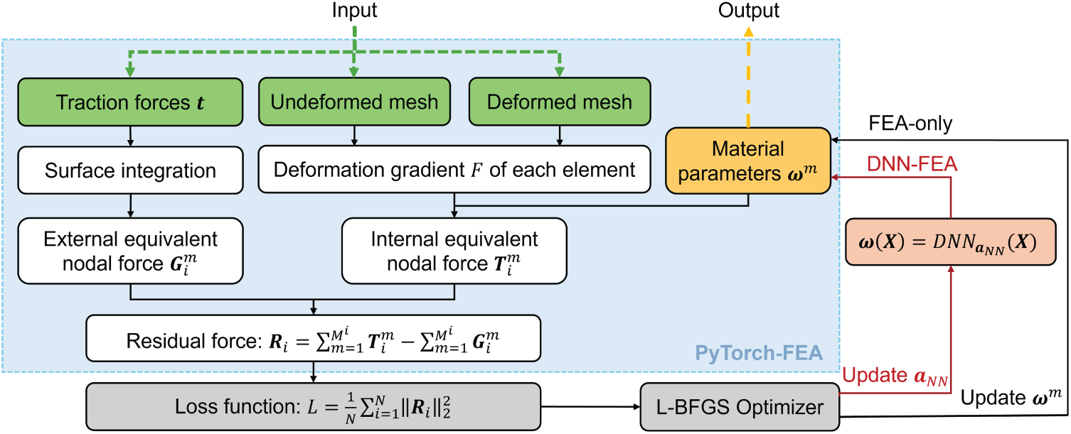
Figure 1: Overview of the workflows for the FEA-only method in PyTorch and DNN-FEA integration strategy

2.4 DNN-FEA Integration for Inverse Material Parameter Identification

The optimization problems associated with identification of nonlinear hyperelastic material parameters often encounter difficulties known as local optima, i.e., multiple sets of material parameters can yield similar near-minimal loss values [46]. This challenge is amplified in heterogeneous material parameter identification due to the large number of unknowns (number of parameters in the constitutive model × number of elements). The problem is further complicated by input noise, such as noises resulting from medical image modalities [47], which propagates to the deformed and undeformed geometries.

To address these issues and mitigate the impact of heterogeneous unknown fields, traditional approaches often incorporate regularization terms (e.g., L1 and L2 regularization or smoothness-based priors) into the loss function to penalize large spatial parameter differences and enforce smoothness [48–50]. However, these explicit penalty terms regularize the solution toward prior assumptions such as smoothness of the identified material parameter fields.

In this study, we employed a DNN-FEA integration strategy to regularize the material parameter field without relying on explicit priors. Specifically, a multilayer perceptron (MLP) was used as a universal function approximator to represent the spatial distribution of constitutive parameters as a function of the undeformed reference coordinates X, i.e.,

ω(X)=DNNaNN(X)(18)

where aNN represents the MLP learnable parameters. Therefore, the material parameters for each element, ωm, can be computed at the center of element m, X¯m. Instead of solving for the parameters independently at each element, the MLP weights are updated to represent the spatial distribution of parameters. According to the universal function approximation theorem, a properly constructed MLP can approximate any spatial distribution function, which provides a flexible regularization effect without prescribing explicit priors.

In the DNN-FEA inverse workflow, the same loss function based on FEA nodal residual force (Eq. (17)) was employed without the need for additional regularization terms,

L(aNN)=1N∑i=1N‖Ri‖22(19)

The ability of DNN to regularize parameter distributions arises from its continuous differentiability, which inherently links the material parameters of adjacent elements within the MLP. Since ω is expressed as a function of aNN, the loss function is consequently also a function of these weights. As shown in Fig. 2, the DNN was used to compute material parameters at each element ωm. A sinusoidal activation function was used in the MLP. The network architecture (number of layers and units per layer, and activation function) was selected via grid search. The learnable parameters aNN are optimized by minimizing the loss function (Eq. (19)) using the L-BFGS algorithm. Training proceeds until the maximum parameter difference between successive epochs falls below a termination tolerance (e.g., 10−10). In this study, DNN training was performed on the Nvidia A800 GPU.

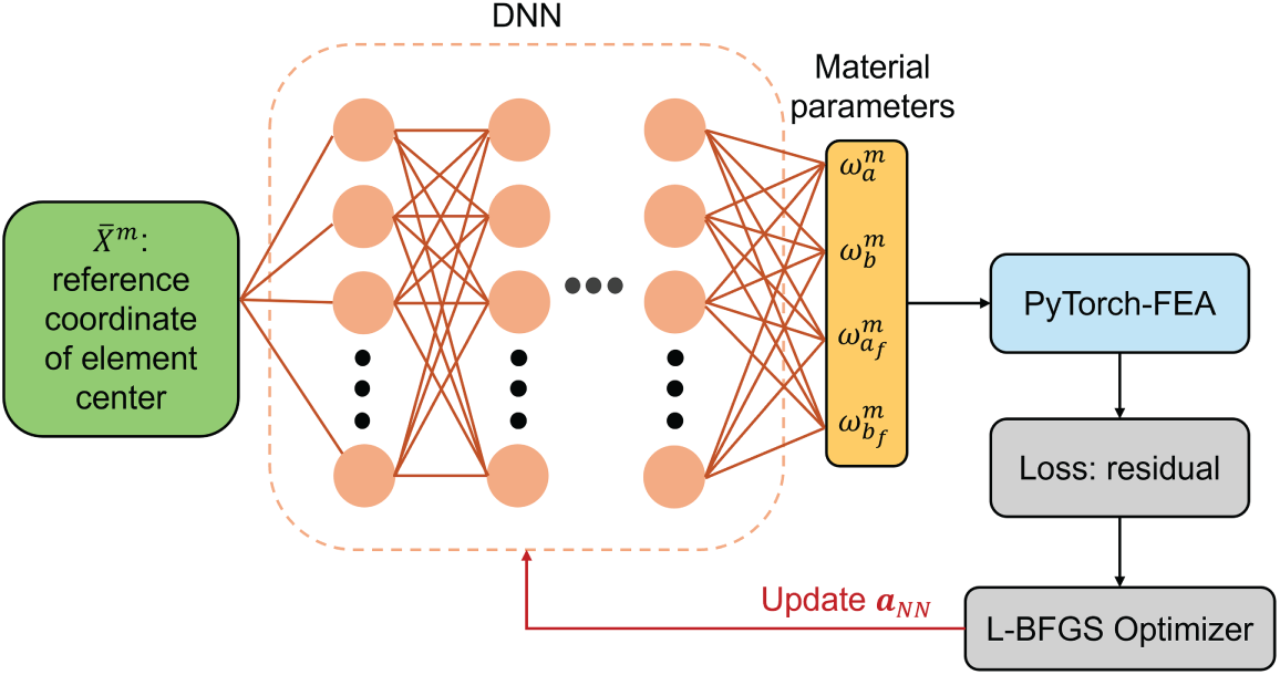
Figure 2: Neural network architecture of the DNN-FEA framework. A multilayer perceptron model was employed to represent the spatial distribution of constitutive parameters as a function of the undeformed reference coordinates

3  Numerical Validations

The proposed DNN-FEA framework is designed for inverse material parameter identification in a variety of cardiovascular applications, including the identification of passive material parameters of the left ventricular (LV) myocardium. During cardiac cycles, the LV exhibits both active and passive mechanical responses. However, in the diastolic phase, myocardial active contraction is minimal, and the LV deforms primarily due to passive filling with blood. Consequently, the end-diastolic pressure-volume relationship (EDPVR) [22,51] is widely regarded as a key descriptor of the LV’s passive mechanical properties. At the onset of diastole, LV pressure is near zero. As the mitral valve opens, blood enters the ventricle, leading to passive myocardial deformation. This passive filling process culminates at end diastole, when the ventricular pressure reaches its peak value under passive conditions [22].

In this work, we demonstrate the application of the proposed DNN-FEA integration approach for identifying passive LV material parameters during diastolic filling. The method was numerically validated using synthetic data generated from forward FEA simulations with two predefined heterogeneous material parameter distributions (referred to as Distributions 1 and 2). Specifically, the LV geometry at the early-diastolic phase was derived from a patient’s multiphase electrocardiogram (ECG)-gated CT scans, which was considered as the undeformed configuration. A representative ground-truth heterogeneous material parameter distribution (Distribution 1 or 2) was then assigned to the undeformed LV. Subsequently, the undeformed geometry was subjected to pressurization up to the end-diastolic phase using forward FEA simulations implemented in PyTorch, which yielded the deformed LV geometry. The undeformed and deformed geometries thus served as inputs for inverse material parameter identification, while the ground-truth material parameter distribution was available for evaluating performance. For DNN-FEA, Distribution 1 was used to perform the DNN grid search to select the best-performing architecture. The DNN-FEA framework with the selected architecture was then applied to identify the material parameter distribution in Distribution 2, and its performance was subsequently evaluated. The details of synthetic data generation are described in the following sections.

3.1 Ground-Truth Undeformed Geometry

In a previous study, we retrospectively collected pre-surgical ECG-gated cardiac CT images from a patient with aortic stenosis who subsequently underwent transcatheter aortic valve replacement (TAVR). We developed a deformation-based deep learning framework, namely DeepCarve (Deep Cardiac Volumetric Mesh) [52], to automatically generate patient-specific volumetric meshes for FEA-based TAVR deployment simulations. In the present study, the DeepCarve framework was used to generate a surface mesh of the patient’s left ventricle (LV) at the early-diastolic phase from the patient-specific CT scans. Since this is the phase when diastolic filling has just begun and the intraventricular pressure is typically near zero, the geometry was considered to represent the undeformed, zero-pressure reference state for subsequent analyses.

The LV surface geometry was cut at both the mitral and aortic annuli and represented by triangular elements. To convert the surface mesh into a volume mesh, tetrahedral elements were employed to fill the LV myocardium. However, 4-node linear tetrahedral elements are unsuitable for nonlinear large-deformation FEA because they lead to a constant deformation gradient within each element [53,54]. Therefore, following surface mesh generation, the LV volume mesh was constructed using 10-node quadratic tetrahedral elements generated by using the ‘tetra mesh’ tool in Altair HyperMesh, which are well suited for large deformation analysis. Finally, fiber orientations representing a simplified myocardial architecture were defined on the undeformed LV volume mesh. Myofibers were assumed to be aligned circumferentially, which represents the orientation of mid-wall fibers. The sheet-normal direction was defined as the surface normal of the outer LV wall, and the sheet direction was computed as the cross product of the myofiber and sheet-normal directions.

3.2 Heterogeneous Ground-Truth Material Property Distributions

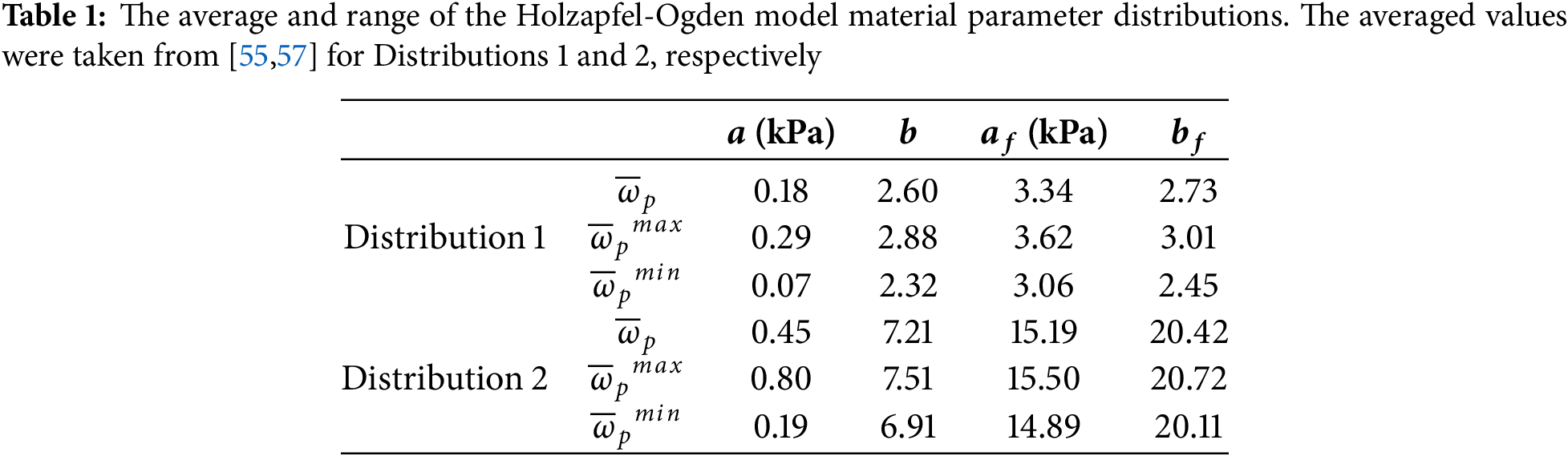
Synthetic heterogeneous material property distributions (Distributions 1 and 2) were assigned to the undeformed LV geometry to generate the deformed end-diastolic configuration. A cylindrical coordinate system was employed to define the spatial variation of material parameters, which were assumed to vary along the circumferential (θ) and axial (z) directions but remain constant along the radial, thickness (r) direction. To represent typical spatial nonuniformity [55], periodic patterns were introduced into the material parameter distributions using a summation of sinusoidal functions. The following distribution was used for Distribution 1:

ωp(z,θ)=ω¯p+λ(sin⁡10θ)(0.2sin⁡(z)+0.3sin⁡(0.1z)+0.5sin⁡(0.01z)(20a)

where ωp (a=1,2,3,4) is one of the material parameters (a,b,af,bf). ω¯p denotes the baseline material parameters, which were derived from MRI-based measurement of healthy human subjects in a previous study [56] and are shown in Table 1. λ is a tunable constant controlling the amplitude of the periodic fluctuations, which was adjusted to ensure that ω is always positive. For Distribution 1, λ was set to be 0.2, −0.5, 0.5, −0.5, respectively, for a,b,af,bf. The resulting range of ωp is shown in Table 1. Similarly, Distribution 2 was generated to represent slightly larger spatial patterns:

ωp(z,θ)=ω¯p+λ(sin⁡5θ)(0.2sin⁡(0.5z)+0.3sin⁡(0.1z)+0.5sin⁡(0.01z)(20b)

where ω¯p was derived from cyclic simple shear experiments of porcine heart tissues [57]. λ was set to be 0.5, −0.5, 0.5, −0.5, respectively, for a,b,af,bf in Distribution 2 to enforce that ω is always positive. The resulting range of ωp in Distribution 2 is also shown in Table 1.

3.3 Generation of Ground-Truth Deformed Geometry Using forward FEA

Starting from the undeformed LV geometry derived from patient CT scans and the assigned heterogeneous material property distribution, a forward finite element simulation was performed to generate the deformed end-diastolic LV geometry under a uniform intraventricular pressure. The pressure was set to P=30 mmHg consistent with typical values of healthy and diseased individuals [22]. The forward FEA simulation was implemented using PyTorch (Fig. 3). Briefly, forward FEA computed the nodal displacements ui(t) by minimizing the residual force (Eq. (16)) as loss in each pseudo time step t. The intraventricular pressure was gradually ramped to 30 mmHg, such that at step t, P(t)=t⋅P. Convergence at each time step was considered achieved when the ratio between maximum residual nodal force and averaged internal equivalent nodal forces fell below the prescribed tolerance of 0.005. If the solution failed to converge at a given time step, the pseudo-time increment was adaptively reduced and the displacement solution ui(t) was reattempted. For displacement boundary conditions, all nodes located on the mitral and aortic annuli were constrained in all degrees of freedom throughout the simulation.

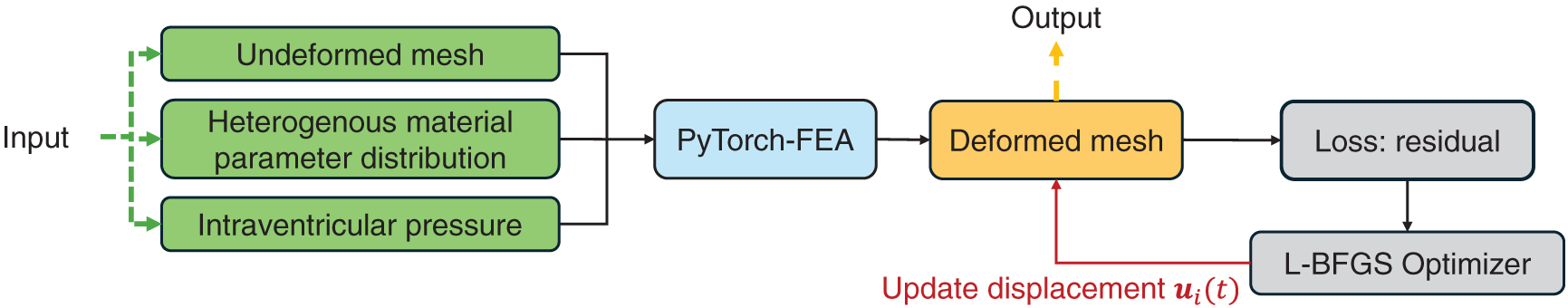
Figure 3: Generation of ground-truth deformed geometry using forward FEA in PyTorch

3.4 Inverse Identification of Heterogeneous LV Material Parameters from Deformed and Undeformed Geometries

For validation, both FEA and DNN-FEA were employed to identify heterogeneous passive material parameters of the left ventricle (LV) from the undeformed and deformed geometries. The identified material parameter distributions obtained from FEA and DNN-FEA were compared against the ground-truth distributions used to generate the geometries. To quantitatively evaluate the accuracy of the inverse identification, the average and maximum relative errors of each HO material parameter, denoted as ωp, were computed across all elements:

εpm=|ω^pm−ωpm|ω¯p(21)

εpavg=1M∑m=1M|ω^pm−ωpm|ω¯p(22)

εpmax=max|ω^pm−ωpm|ω¯p(23)

where ω^pm and ωpm represent the identified and ground-truth parameters of element m, respectively, and ω¯p=1M∑m=1Mωpm denotes the mean ground-truth parameter across all elements.

To further compare the identified and ground-truth mechanical responses, stress-strain curves were generated under simulated biaxial loading conditions using both the identified and ground-truth material parameters. Three stretch-controlled loading protocols were considered, varying the ratio between myofiber strain (Eff) and sheet (Ess) strain as Eff:Ess=0.5,1,2. The corresponding Cauchy stress and Green strain responses were visualized in the myofiber and sheet directions. Performance was quantified by first generating stress-strain curves based on the average identified parameters (ω¯^) and the average ground-truth parameters (ω¯) material parameters. Additionally, stress-strain curves were simulated for representative spatial locations within the LV geometry to illustrate local variations in model performance.

3.5 Optimizer Configuration

Both the FEA-only and DNN-FEA inverse solvers were optimized using the L-BFGS algorithm implemented in PyTorch [58,59]. The following hyperparameters were used in the numerical validation: history size = 20, line-search type = strong Wolfe, maximum iterations per step = 1, gradient tolerance = 1×10−10, parameter-change tolerance = 1×10−10, and learning rate = 1.0. No preconditioning was used. The L-BFGS optimization procedure is fully deterministic.

4  Results

4.1 Grid Search

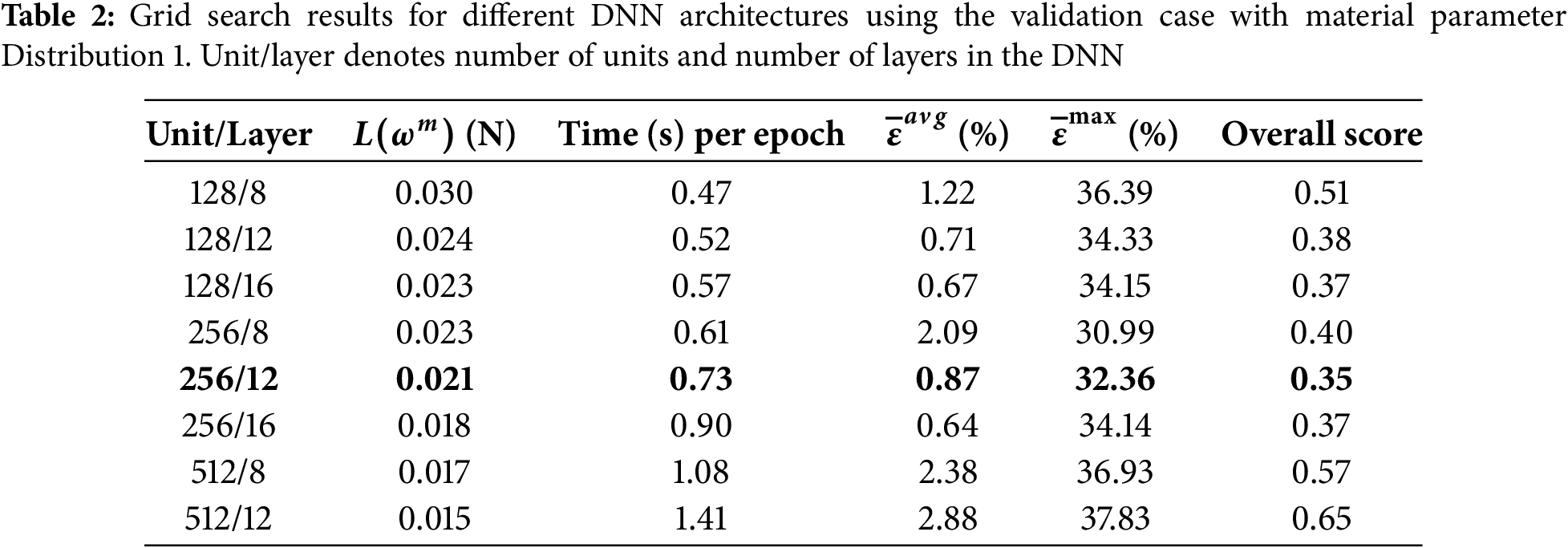
To determine the optimal MLP architecture for the DNN-FEA inverse approach, a grid search was performed by varying both the number of hidden layers and the number of units per layer using validation data with Distribution 1. The results of this search are summarized in Table 2. The best-performing DNN architecture was selected based on the following four criteria: (1) the minimized loss function value (total residual forces), (2) computation time per epoch, (3) the average error ε¯avg, and (4) maximum error ε¯max across all material parameters. To balance these trade-offs, an overall score was calculated by normalizing each criterion between its minimum and maximum values and then summing the normalized criteria. Based on this evaluation, the final architecture selected consisted of 12 hidden layers with 256 units per layer. This DNN architecture was applied to identify heterogenous material parameters in Distribution 2.

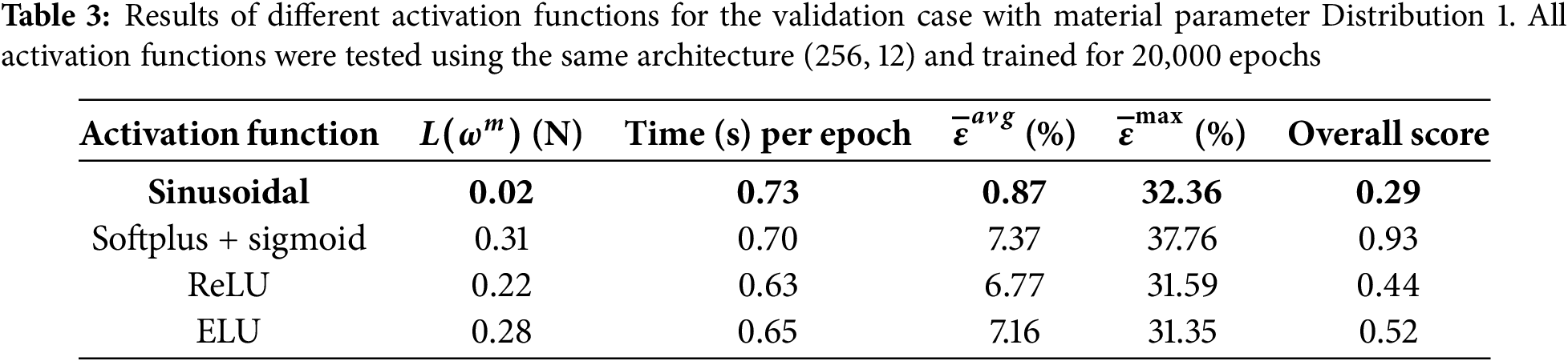
Several activation functions (sinusoidal, softplus with sigmoid in the output layer, ReLU, and ELU) were compared using the best-performing DNN architecture. As shown in Table 3, the sinusoidal activation function achieved the best overall score and was retained for subsequent analysis.

4.2 Spatial Material Parameter Distribution (Distribution 1)

Both the FEA and DNN-FEA approaches were applied to the numerical validation dataset with Distribution 1. The identified spatial distributions of the four material parameters are shown in Fig. 4, alongside the ground-truth distributions. While FEA produced parameter fields with similar spatial patterns resembling the ground truth, noticeable deviations in parameter values were observed. These discrepancies are likely attributable to local optima in the optimization of the loss function. In contrast, DNN-FEA yielded spatial fields that were visually much closer to the ground truth for all parameters. Quantitative evaluation is summarized in Table 4, which reports the average and maximum errors for each parameter. The largest errors were observed for parameter a, where FEA produced errors several times higher than those of the other parameters. By comparison, DNN-FEA consistently maintained average errors below 2.2%, which demonstrated substantially greater accuracy. Fig. 5 further illustrates the spatial error distributions for each parameter. Overall, the closer agreement with ground truth distribution and the lower errors indicate that the DNN-FEA framework consistently outperformed the FEA method.

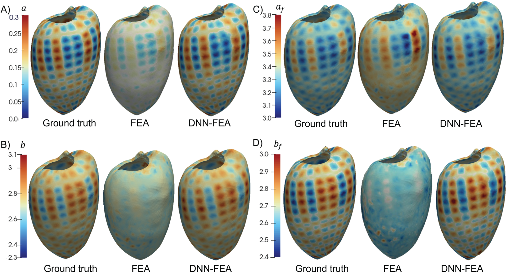
Figure 4: Comparison of identified and ground truth material parameter distributions (Distribution 1) on the deformed end-diastolic LV geometry: (A) distribution of a. (B) distribution of b. (C) distribution of af. (D) distribution of bf

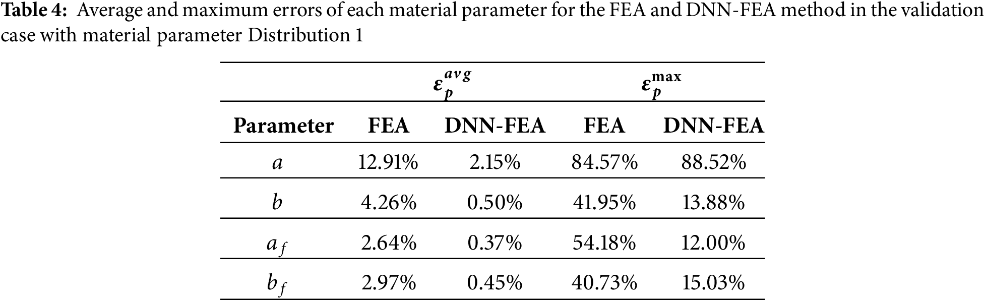
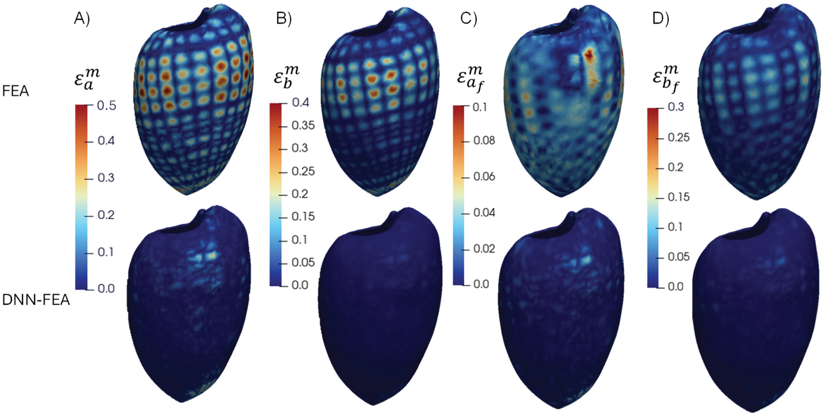
Figure 5: Spatial distributions of the error of each material parameter (Distribution 1) for the FEA and DNN-FEA methods on the deformed end-diastolic LV geometry: (A) distribution of a. (B) distribution of b. (C) distribution of af. (D) distribution of bf

4.3 Loss Function Convergence

To further investigate the mechanism behind the superior performance of DNN-FEA in the validation case with material parameter Distribution 1, we visualized the residual force-based loss function values and the average errors εpavg of each material parameter during the solution process over 20,000 epochs for both the FEA and DNN-FEA methods. The results are shown in Fig. 6. For all four parameters, DNN-FEA exhibited a steady reduction in loss values, accompanied by a progressive and consistent decrease in average parameter error following the same trend. In contrast, the FEA method showed an inconsistent reduction in average error, even though the loss function decreased quickly to a small value. For parameters b and bf, the average error initially increased slightly before decreasing. This discrepancy between residual force loss and parameter error suggests that the FEA-only solution was likely trapped in local optima. These findings demonstrate that DNN-FEA provides an effective regularization effect in inverse material parameter identification, which helped to avoid suboptimal solutions.

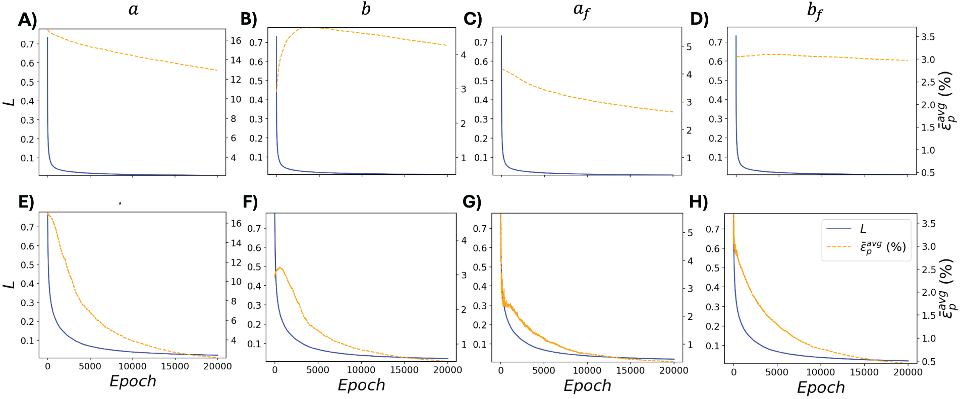
Figure 6: Training loss and average error over 20,000 epochs for each material parameter in the validation case with material parameter Distribution 1. Panels (A–D) correspond to the FEA method, and panels (E–H) correspond to the DNN-FEA method

4.4 Stress-Strain Responses

To evaluate the identified myocardial mechanical response against the ground-truth response in the validation case with material parameter Distribution 1, we simulated stress-strain behaviors in both the myofiber and sheet directions. Fig. 7 compares the stress-strain curves obtained using the spatially averaged material parameters ω¯^ identified by the FEA and DNN-FEA methods, identified by the FEA and DNN-FEA methods, as well as those obtained from the spatially averaged ground-truth parameters ω¯, under three biaxial strain ratios between the myofiber and sheet directions (0.5, 1.0, and 2.0). The DNN-FEA model showed a closer match to the ground-truth response, while the FEA average response also agreed reasonably well.

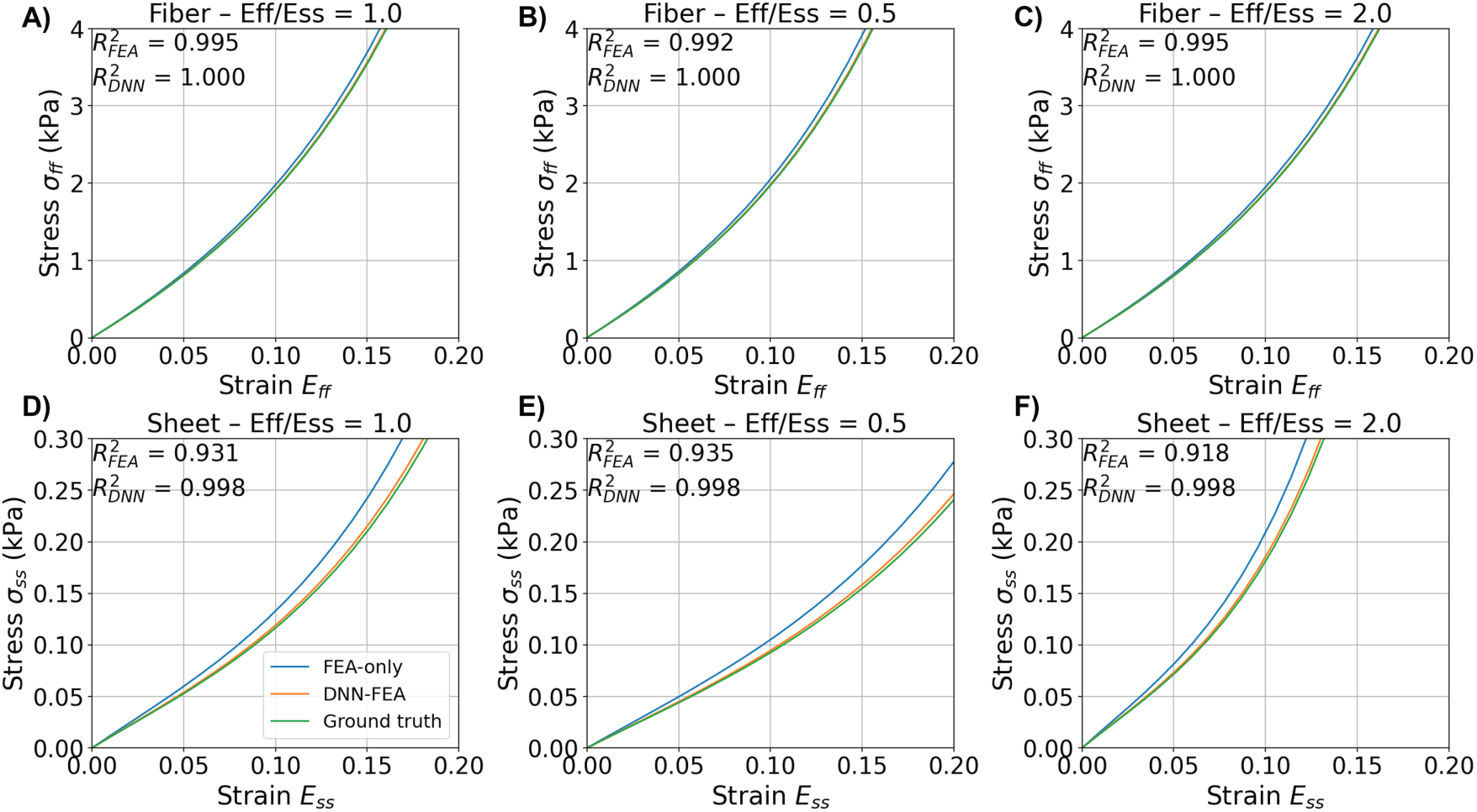
Figure 7: Comparison of identified stress-strain responses under various strain ratios using FEA-identified, DNN-FEA-identified, and ground truth spatially-averaged material parameters in the validation case with material parameter Distribution 1. (A–C) show the fiber-direction stress-strain curves (σff vs. Eff) for increasing strain ratios (Eff/Ess = 0.5, 1.0, and 2.0), while (D–F) show the corresponding sheet-direction responses (σss vs. Ess)

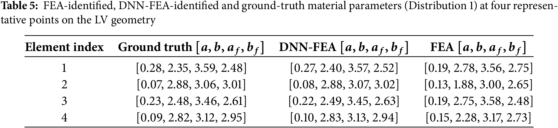
To compare heterogeneous mechanical responses at different spatial locations in the validation case with material parameter Distribution 1, Fig. 8 shows equibiaxial stress-strain curves at four representative elements on the LV geometry. At elements 1, 2, and 4, DNN-FEA more closely matched the ground-truth curves in both the myofiber and sheet directions compared to FEA. At element 3, FEA slightly outperformed DNN-FEA in the sheet direction, while DNN-FEA achieved a better match in the fiber direction. Across all sampled locations, DNN-FEA closely approximated the ground-truth responses, with R2 > 0.942, whereas FEA showed weaker agreement, particularly in the sheet direction (R2 = −0.617 and 0.100 at element 1 and 2). The corresponding material parameters at these locations are listed in Table 5. These results confirm that DNN-FEA yields identified estimates closer to ground-truth values and more effectively captures spatially varying material properties.

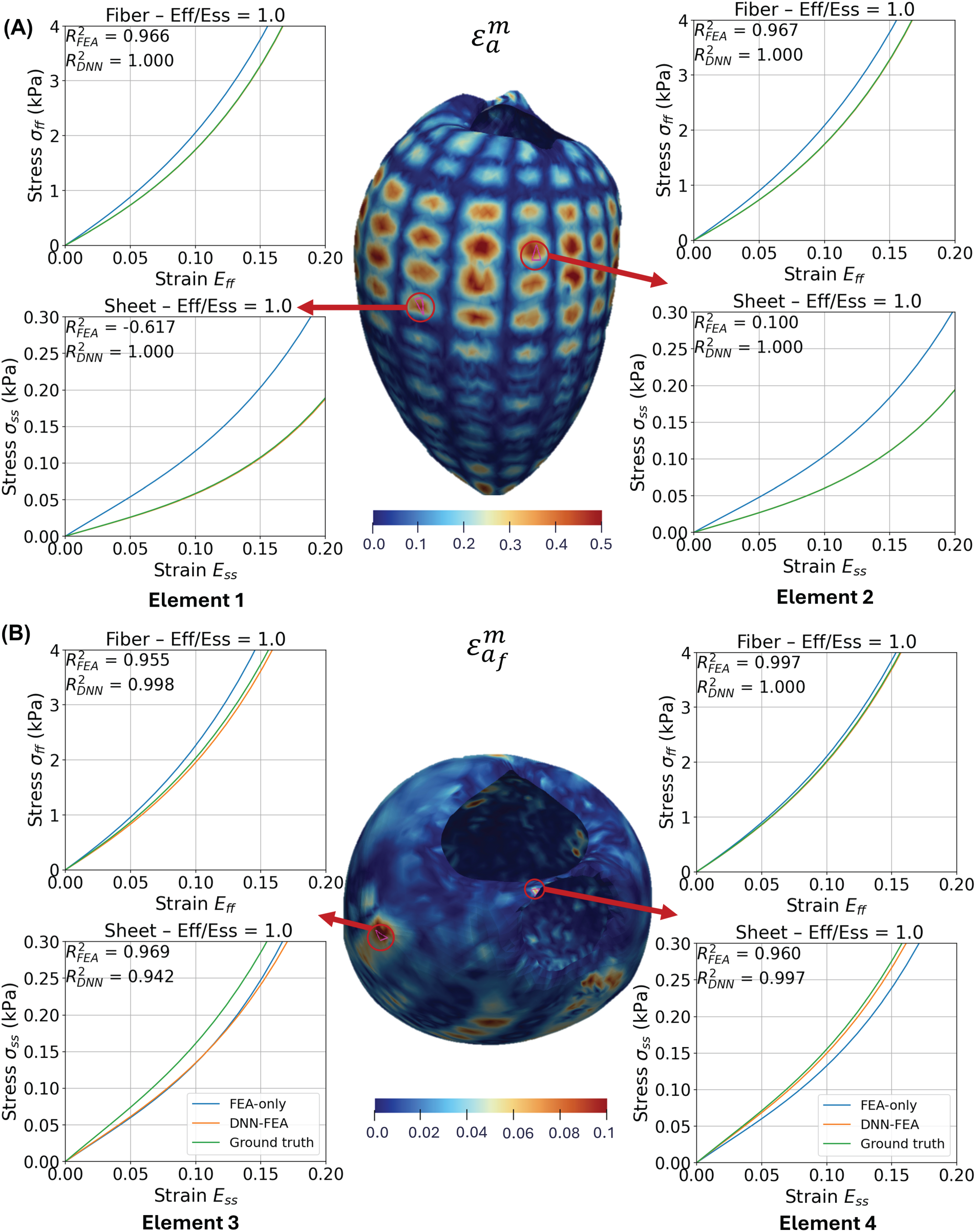
Figure 8: Equibiaxial stress-strain curves at four representative points on the deformed end-diastolic LV geometry using the FEA-identified, DNN-FEA-identified and ground-truth material parameters (Distribution 1). Error distributions (a and af) for the FEA method were shown. (A) Elements 1 and 2; (B) Elements 3 and 4

4.5 Validation Case with Material Parameter Distribution 2

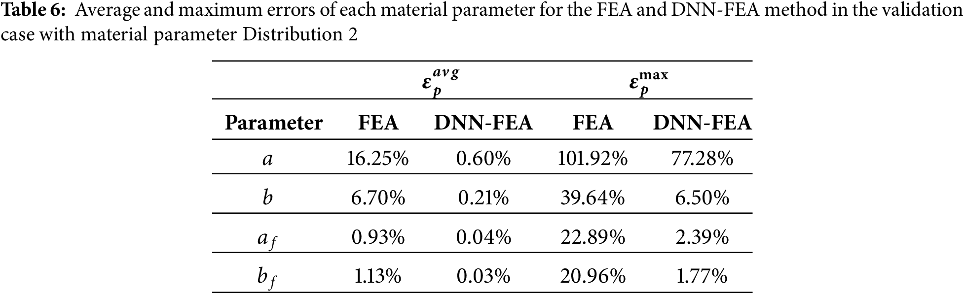
Using the DNN architecture identified through grid search with material parameter Distribution 1, the DNN-FEA framework was applied to the numerical validation dataset with material parameter Distribution 2 to identify heterogeneous material properties. For comparison, the FEA method in PyTorch was also included. The identified spatial distributions of the four material parameters obtained by FEA, DNN-FEA, and the ground truth are shown in Fig. 9. As illustrated in Fig. 10, DNN-FEA achieved close agreement with the ground truth, whereas the FEA method produced noticeable errors. Table 6 further demonstrated that DNN-FEA resulted in substantially lower average and maximum errors for each parameter compared to FEA. These results demonstrate that the DNN architecture obtained through grid search may be applied to identify different spatial material property distributions.

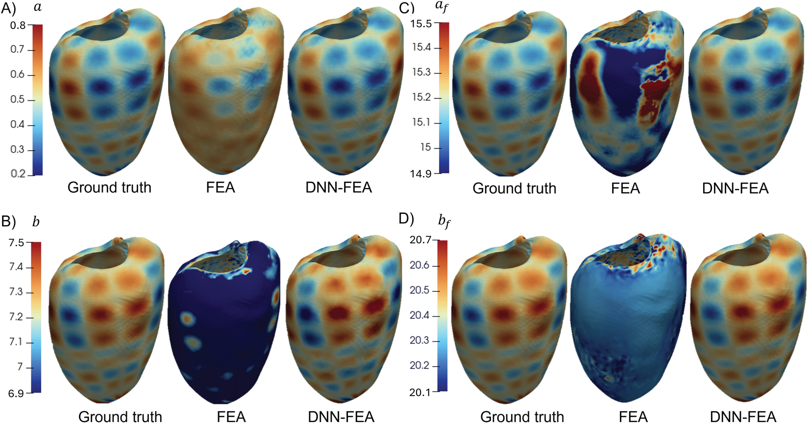
Figure 9: Comparison of identified and ground truth material parameter distribution (Distribution 2) on the deformed end-diastolic LV geometry: (A) distribution of a. (B) distribution of b. (C) distribution of af. (D) distribution of bf

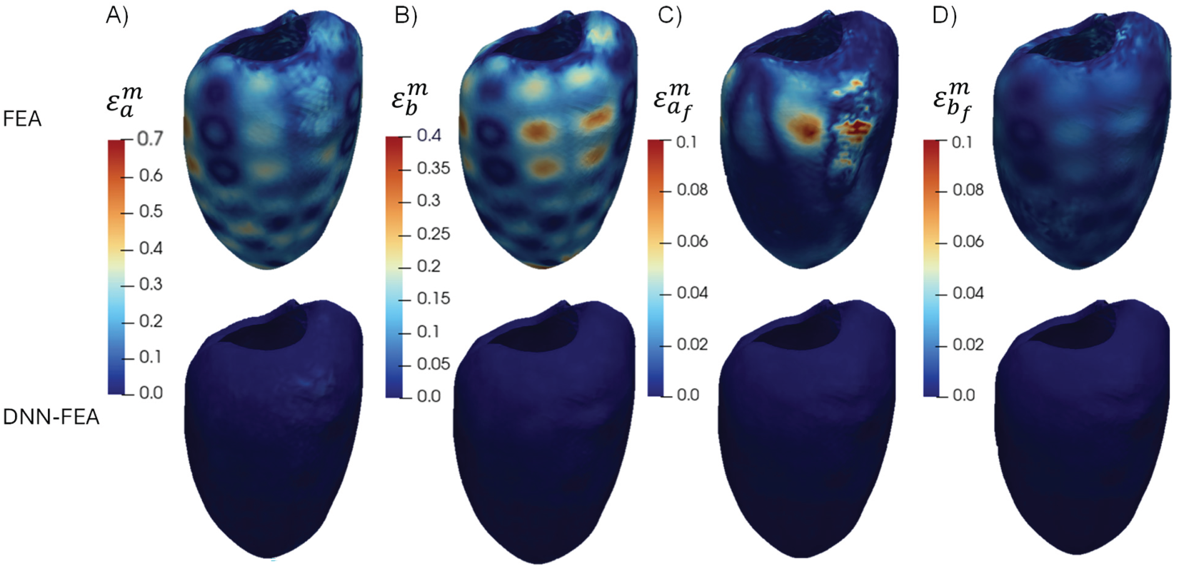
Figure 10: Spatial distributions of the error of each material parameter (Distribution 2) for the FEA and DNN-FEA method on the deformed end-diastolic LV geometry: (A) distribution of a. (B) distribution of b. (C) distribution of af. (D) distribution of bf

4.6 Sensitivity Analyses

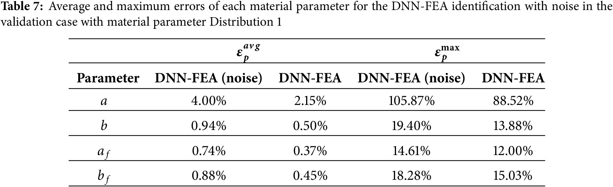
To assess the performance of the proposed inverse DNN-FEA framework under noisy conditions, we performed an additional experiment using deformed geometry with Gaussian noise. Noise was introduced during the forward FEA simulation by applying non-uniform pressure loading, in which spatially varying noises were added to the uniform intraventricular pressure (P = 30 mmHg) with 1% standard deviation. The undeformed and noisy deformed geometries were then used as inputs for inverse identification using the same DNN-FEA configuration and hyperparameters as in case 1. Fig. 11 summarizes the identified material parameters under noisy inputs. Table 7 demonstrates that the DNN-FEA framework achieves relatively low εpavg across all 4 material parameters.

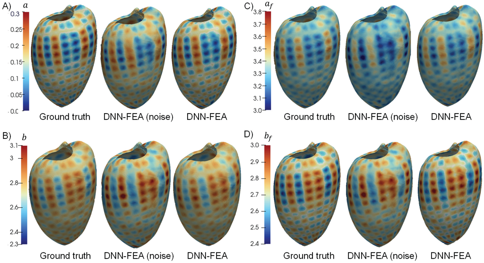
Figure 11: Comparison of identified and ground truth material parameter distribution (Distribution 1 with noise) on the deformed end-diastolic LV geometry: (A) distribution of a. (B) distribution of b. (C) distribution of af. (D) distribution of bf

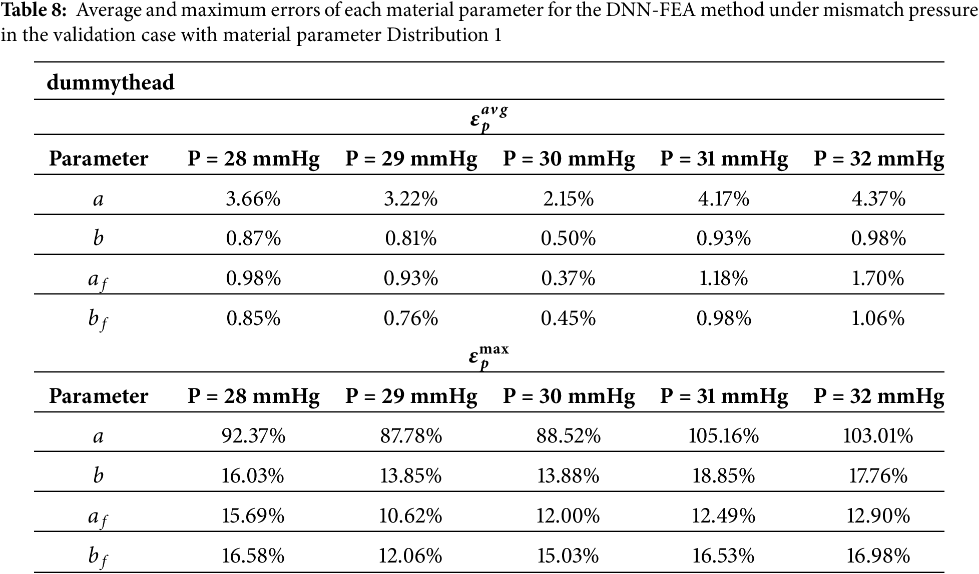
To quantify the sensitivity of the DNN-FEA workflow to pressure mismatch, we repeated the inverse identification process using uniform pressures of 28, 29, 31, and 32 mmHg as inputs, while keeping the same input geometries generated under a pressure of 30 mmHg. Quantitative comparisons are summarized in Table 8. These results demonstrate that small pressure mismatches (±1–2 mmHg) do not significantly degrade the performance of the proposed framework.

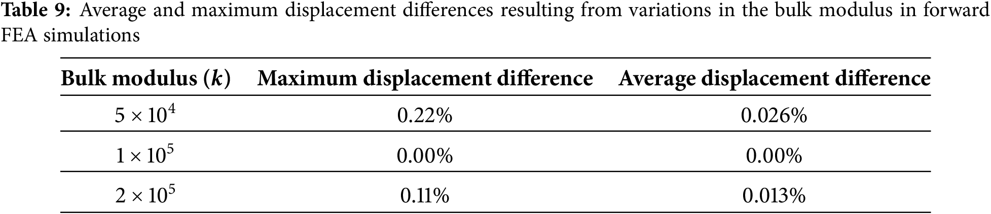
An additional sensitivity analysis was performed using bulk modulus values of k=5×104 and k=2×105 in forward FEA simulations. The resulting differences in displacement were quantified relative to the case with k=1×105. The results, summarized in the Table 9, indicate that the FEA outcomes are nearly independent of the specific choice of k.

5  Discussion

In this study, we developed a DNN-FEA framework for the inverse identification of heterogeneous passive constitutive parameters of the left ventricular myocardium. In this novel formulation, a DNN was employed as a regularizer to approximate the spatial distribution of material parameters based on the reference coordinates. Our results demonstrate that this DNN-FEA integration strategy significantly improves inverse material parameter identification compared to classical FEA formulations implemented in PyTorch. The average errors between the identified parameters and the ground truth were substantially lower with DNN-FEA (case 1: 0.37%~2.15%; case 2: 0.03%~0.60%) than with FEA without DNN (case 1: 2.64%~12.91%; case 2: 0.93%~16.25%). The results suggest that this framework has the potential to accurately identify spatial material property distributions. These promising numerical validation results highlight the potential of integrating state-of-the-art deep learning capabilities to enhance classical computational mechanics toolkits, rather than replacing them entirely. The DNN-FEA workflow may further pave the way for noninvasive identification of pathological regions in the myocardium from clinical images. Nevertheless, rigorous experimental and clinical validation is warranted in future work.

In general, identifying heterogeneous nonlinear constitutive parameters from in vivo clinical data is highly challenging [12,13], and therefore requires specialized inverse optimization workflows [46,60] or data-driven approaches [15,17]. This is not only because the underlying error/loss function can be non-convex with multiple local optima, but also because the unknowns consist of multiple three-dimensional, spatially varying material parameter fields, making the solution space extremely large [48]. In our numerical validation cases, the model contained 153,467 10-node quadratic tetrahedral elements, resulting in a total of 153,467 × 4 = 613,868 unknown material parameters. Even when using state-of-the-art optimization methods such as L-BFGS, directly solving for these unknowns individually via the loss function in Eq. (17) can lead to solution being stuck at local optima, as shown in the FEA-only scenario. Our results demonstrated that embedding a DNN within the FEA workflow regularizes the material parameter distribution, effectively constraining the solution space and thereby facilitating the identification of unknown constitutive parameters. Unlike traditional regularization strategies that add explicit penalty terms to the loss function (e.g., L1/L2 or smoothness constraints), which could guide the solution toward prior assumptions such as smoother spatial fields [48–50], the DNN-FEA integration strategy preserves the same loss function as FEA. Instead, it leverages the DNN as a universal function approximator to represent the spatial distribution of constitutive parameters in a more flexible manner, without imposing explicit priors. In our demonstrative application, the DNN-FEA integration approach predicted the spatial distributions of passive myocardial material parameters with consistently lower errors and better agreement with ground-truth stress-strain behavior. Compared with the classical FEA method implemented in PyTorch, which estimates material parameters independently for each element, the DNN-FEA approach offers a more suitable and robust solution for complex 3D inverse problems involving spatially heterogeneous constitutive parameters.

In large-deformation solid mechanics problems, computing the deformation gradient requires differentiating the deformed configuration with respect to the reference configuration. In a typical PINN setup, a neural network serves as a function approximator to predict the deformed configuration x from the reference configuration X, e.g., x=fDNN(X). Hence, F=∂fDNN(X)∂X. In this setup, even small perturbations in X can produce considerable changes in F, which could lead to instability. Moreover, because the PINN loss function is formulated directly from the continuous static equilibrium equations (e.g., Eq. (13)) without discretization, the backpropagated deformation gradients can introduce numerical instabilities and slow convergence, as reported in recent studies [35,36,61]. Consequently, PINNs may be unsuitable for complex 3D inverse identification problems in myocardium. In contrast, FEA computes the deformation gradient tensor by differentiating the shape functions with respect to element coordinates (Eq. (11)), thereby avoiding reliance on automatic differentiation for F and preventing the propagation of such instabilities. Therefore, we argue that integrating DNNs into the FEA framework may offer a more robust strategy for inverse hyperelasticity problems, which could effectively mitigate the instability issues associated with deformation gradient computation in PINNs.

Our current work has several limitations. (1) We employed a reduced form of the Holzapfel-Ogden (HO) model with four parameters following a recent study [22], which may not fully capture the complex mechanical behavior of the myocardium, particularly the shear behavior typically represented by the invariant I8. We acknowledge that including shear and cross-fiber coupling terms in the constitutive model would provide a more comprehensive description of myocardial mechanical behavior [62]. When using the reduced form, the inverse analysis in this study may have limited capability to capture deformations associated with shear and cross-fiber interactions. Consequently, the mechanical behavior identified using the reduced model should be interpreted primarily as an approximation of the extensional response. When applying this framework to clinical data, care must be taken in interpreting the results, as shear and cross-fiber coupling effects are not represented in the constitutive model. However, for inverse material parameter identification, such simplifications have been adopted in previous studies to achieve a balance between parameter identifiability and accurate representation of cardiac deformation [22]. Consequently, simplified Holzapfel-Ogden models are commonly used for inverse identification of myocardial mechanical properties [63,64]. Future work will investigate the feasibility of identifying the full HO model parameters from synthetic data. (2) The DNN architecture was determined using grid search. Applying advanced hyperparameter optimization methods [65] could further enhance network performance. (3) We assumed a simplified myofiber architecture with all fibers oriented circumferentially throughout the LV wall. Previous studies have treated fiber angles as unknown parameters in applications involving blood vessels, largely due to their thin wall thickness and relatively simple fiber architecture, which is dominated by circumferentially aligned collagen fibers with limited dispersion [66]. In contrast, the left ventricular myocardium has a much thicker wall and exhibits highly complex, transmural, helix-to-transverse fiber rotation, involving fiber, sheet, and sheet-normal directions that vary significantly across the ventricular wall [67]. These complex orientations constitute additional heterogeneous fields (tens of thousands of unknowns) and are extremely challenging to identify simultaneously with other material parameters using CT image data alone. In addition, routine clinical noninvasive imaging techniques primarily capture the bulk myocardial volume and lack the resolution to visualize detailed fiber architecture throughout the wall [68,69]. For this reason, most myocardial inverse modeling studies prescribe fiber orientations using rule-based algorithms rather than identifying them as unknowns [67]. Following this common assumption, the present study focuses on demonstrating the proposed framework for heterogeneous material parameter identification, and thus adopts a simplified myofiber orientation. In addition, it appears that most previous studies assume uniform (homogeneous) or region-based material properties at coarser resolutions. Incorporating complex fiber orientations may increase the challenge of heterogeneous parameter identification and warrants further investigation. (4) It is important to note that the successful application of the same MLP architecture to both Distribution 1 and Distribution 2 should be interpreted within the context of these two specific distributions. Future work will evaluate the MLP architecture under more diverse spatial patterns to further assess its generalizability. (5) Numerical validation was performed using a synthetic deformed geometry and material distributions. To enable inverse identification of material properties of real patient data, the key requirement is to obtain the displacement fields at both the external surface and internal volume of the ventricle. This can be achieved by establishing point-to-point mesh correspondence between the early-diastolic and end-diastolic ventricular geometries using non-rigid registration methods (e.g., Deformetrica software [70]), which is often a prerequisite for statistical shape analysis [71]. Once the mesh correspondence is established, displacements at internal nodes can be computed from registered meshes using transformation techniques such as thin-plate spline interpolation [72], thereby providing the displacement field required for the inverse solver. Care must be taken to ensure that the registration process preserves ventricular volume consistency between early-diastolic and end-diastolic geometries, which is necessary for the nearly incompressible constitutive formulation. This may be achieved by incorporating volume-preserving regularization into the registration procedure. (6) Experimental validation is needed to more comprehensively assess identification performance. For example, ex vivo myocardial tissue could be imaged under zero-load and known pressure conditions using micro-CT. The proposed DNN-FEA framework could then be applied to identify heterogeneous material properties, and mechanical tests such as biaxial tensile and simple shear experiments could be used to obtain ground-truth material parameters for validation.

In the presence of noise arising from image segmentation errors, partial volume effects, and uncertainty in boundary conditions in real patient data, one potential failure mode is that noise may amplify the incompressibility term in the constitutive formulation and obscure the isochoric response during inverse identification. One mitigation strategy is to introduce additional constraints in the mesh-registration cost function to penalize volume differences between early-diastolic and end-diastolic geometries. Additional penalties for preserving element quality may also help mitigate other types of noise and facilitate the DNN-FEA inverse identification process. Methods such as volume-preserving registration [73] and mesh smoothing [74] could also be employed. Future studies will investigate these failure modes associated with inverse identification of material parameters and the mitigation strategies.

6  Conclusion

We developed a DNN-FEA framework that integrates a DNN as a regularizer to approximate the spatial distribution of material parameters, enabling accurate identification of heterogeneous myocardial properties. Our results demonstrate that DNN-FEA outperformed traditional FEA formulations implemented in PyTorch, which yielded substantially lower average errors in the identified parameters compared to the ground truth (case 1, DNN-FEA: 0.37%~2.15% vs. FEA: 2.64%~12.91%). The results suggest that the same DNN architecture is capable of identifying a different spatial material property distribution (case 2, DNN-FEA: 0.03%~0.60% vs. FEA: 0.93%~16.25%). In future work, the DNN-FEA strategy may pave the way for the identification of heterogeneous myocardial material parameters from in vivo clinical imaging data. The inverse workflow could also be extended to other biomechanical simulation applications.

Acknowledgement: None.

Funding Statement: This work was supported in part by the National Science Foundation under Grants DMS 2436630 and 2436629.

Author Contributions: The authors confirm contribution to the paper as follows: Conceptualization, Minliang Liu, Daniel H. Pak, James S. Duncan, Liang Liang; methodology, Liang Liang, Daniel H. Pak, Minliang Liu, Zhuofan Li; software, Liang Liang, Minliang Liu, Zhuofan Li; validation, Zhuofan Li, Minliang Liu; formal analysis, Zhuofan Li; investigation, Zhuofan Li; resources, Daniel H. Pak, James S. Duncan, Liang Liang, Minliang Liu; data curation, Daniel H. Pak; writing—original draft preparation, Minliang Liu, Zhuofan Li; writing—review and editing, Minliang Liu, Zhuofan Li; visualization, Zhuofan Li, Minliang Liu; supervision, Minliang Liu, Liang Liang, James S. Duncan; project administration, Minliang Liu, Liang Liang; funding acquisition, Minliang Liu, Liang Liang. All authors reviewed the results and approved the final version of the manuscript.

Availability of Data and Materials: The full source code for the DNN-FEA inverse material parameter identification framework is publicly available at: https://github.com/zhuofli/DNN_FEA. The clinical CT imaging data and the left-ventricular geometries will be available upon reasonable request to the corresponding author, subject to institutional approvals.

Ethics Approval: Not applicable.

Conflicts of Interest: The authors declare no conflicts of interest to report regarding the present study.

References

1. Szabo B, Babuska I. Finite element analysis: method, verification and validation. Hoboken, NJ, USA: Wiley; 2021. doi:10.1002/9781119426479. [Google Scholar] [CrossRef]

2. Capelli C, Bosi GM, Cerri E, Nordmeyer J, Odenwald T, Bonhoeffer P, et al. Patient-specific simulations of transcatheter aortic valve stent implantation. Med Biol Eng Comput. 2012;50(2):183–92. doi:10.1007/s11517-012-0864-1. [Google Scholar] [PubMed] [CrossRef]

3. Sun W, Martin C, Pham T. Computational modeling of cardiac valve function and intervention. Annu Rev Biomed Eng. 2014;16(1):53–76. doi:10.1146/annurev-bioeng-071813-104517. [Google Scholar] [PubMed] [CrossRef]

4. de Jaegere P, De Santis G, Rodriguez-Olivares R, Bosmans J, Bruining N, Dezutter T, et al. Patient-specific computer modeling to predict aortic regurgitation after transcatheter aortic valve replacement. JACC Cardiovasc Interv. 2016;9(5):508–12. doi:10.1016/j.jcin.2016.01.003. [Google Scholar] [PubMed] [CrossRef]

5. Martin C, Sun W, Elefteriades J. Patient-specific finite element analysis of ascending aorta aneurysms. Am J Physiol Heart Circ Physiol. 2015;308(10):H1306–16. doi:10.1152/ajpheart.00908.2014. [Google Scholar] [PubMed] [CrossRef]

6. Erhart P, Hyhlik-Dürr A, Geisbüsch P, Kotelis D, Müller-Eschner M, Gasser TC, et al. Finite element analysis in asymptomatic, symptomatic, and ruptured abdominal aortic aneurysms: in search of new rupture risk predictors. Eur J Vasc Endovasc Surg. 2015;49(3):239–45. doi:10.1016/j.ejvs.2014.11.010. [Google Scholar] [PubMed] [CrossRef]

7. Lally C, Dolan F, Prendergast PJ. Cardiovascular stent design and vessel stresses: a finite element analysis. J Biomech. 2005;38(8):1574–81. doi:10.1016/j.jbiomech.2004.07.022. [Google Scholar] [PubMed] [CrossRef]

8. Kan X, Ma T, Jiang X, Holzapfel GA, Dong Z, Xu XY. Towards biomechanics-based pre-procedural planning for thoracic endovascular aortic repair of aortic dissection. Comput Meth Programs Biomed. 2024;244(2):107994. doi:10.1016/j.cmpb.2023.107994. [Google Scholar] [PubMed] [CrossRef]

9. Roy D, Holzapfel GA, Kauffmann C, Soulez G. Finite element analysis of abdominal aortic aneurysms: geometrical and structural reconstruction with application of an anisotropic material model. IMA J Appl Math. 2014;79(5):1011–26. doi:10.1093/imamat/hxu037. [Google Scholar] [CrossRef]

10. Gasser TC, Ogden RW, Holzapfel GA. Hyperelastic modelling of arterial layers with distributed collagen fibre orientations. J R Soc Interface. 2006;3(6):15–35. doi:10.1098/rsif.2005.0073. [Google Scholar] [PubMed] [CrossRef]

11. Kyriacou SK, Shah AD, Humphrey JD. Inverse finite element characterization of nonlinear hyperelastic membranes. J Appl Mech. 1997;64(2):257–62. doi:10.1115/1.2787301. [Google Scholar] [CrossRef]

12. Wittek A, Derwich W, Karatolios K, Fritzen CP, Vogt S, Schmitz-Rixen T, et al. A finite element updating approach for identification of the anisotropic hyperelastic properties of normal and diseased aortic walls from 4D ultrasound strain imaging. J Mech Behav Biomed Mater. 2016;58(1):122–38. doi:10.1016/j.jmbbm.2015.09.022. [Google Scholar] [PubMed] [CrossRef]

13. Wittek A, Karatolios K, Bihari P, Schmitz-Rixen T, Moosdorf R, Vogt S, et al. In vivo determination of elastic properties of the human aorta based on 4D ultrasound data. J Mech Behav Biomed Mater. 2013;27:167–83. doi:10.1016/s0021-9290(12)70020-9. [Google Scholar] [CrossRef]

14. Liang L, Liu M, Martin C, Elefteriades JA, Sun W. A machine learning approach to investigate the relationship between shape features and numerically predicted risk of ascending aortic aneurysm. Biomech Model Mechanobiol. 2017;16(5):1519–33. doi:10.1007/s10237-017-0903-9. [Google Scholar] [PubMed] [CrossRef]

15. Liu M, Liang L, Ismail Y, Dong H, Lou X, Iannucci G, et al. Computation of a probabilistic and anisotropic failure metric on the aortic wall using a machine learning-based surrogate model. Comput Biol Med. 2021;137:104794. doi:10.1016/j.compbiomed.2021.104794. [Google Scholar] [PubMed] [CrossRef]

16. Liang L, Liu M, Martin C, Sun W. A machine learning approach as a surrogate of finite element analysis-based inverse method to estimate the zero-pressure geometry of human thoracic aorta. Int J Numer Methods Biomed Eng. 2018;34(8):e3103. doi:10.1002/cnm.3103. [Google Scholar] [PubMed] [CrossRef]

17. Liu M, Liang L, Sun W. Estimation of in vivo constitutive parameters of the aortic wall using a machine learning approach. Comput Meth Appl Mech Eng. 2019;347:201–17. doi:10.1016/j.cma.2018.12.030. [Google Scholar] [PubMed] [CrossRef]

18. Cuomo S, Di Cola VS, Giampaolo F, Rozza G, Raissi M, Piccialli F. Scientific machine learning through physics-informed neural networks: where we are and what’s next. J Sci Comput. 2022;92(3):88. doi:10.1007/s10915-022-01939-z. [Google Scholar] [CrossRef]

19. Sahin T, von Danwitz M, Popp A. Solving forward and inverse problems of contact mechanics using physics-informed neural networks. Adv Model Simul Eng Sci. 2024;11(1):11. doi:10.1186/s40323-024-00265-3. [Google Scholar] [CrossRef]

20. Schönlieb C-B, Shumaylov Z. Data-driven approaches to inverse problems. arXiv:250611732. 2025. [Google Scholar]

21. Arridge S, Maass P, Öktem O, Schönlieb CB. Solving inverse problems using data-driven models. Acta Numer. 2019;28:1–174. doi:10.1017/s0962492919000059. [Google Scholar] [CrossRef]

22. Babaei H, Mendiola EA, Neelakantan S, Xiang Q, Vang A, Dixon RAF, et al. A machine learning model to estimate myocardial stiffness from EDPVR. Sci Rep. 2022;12(1):5433. doi:10.1038/s41598-022-09128-6. [Google Scholar] [PubMed] [CrossRef]

23. Cai L, Ren L, Wang Y, Xie W, Zhu G, Gao H. Surrogate models based on machine learning methods for parameter estimation of left ventricular myocardium. R Soc Open Sci. 2021;8(1):201121. doi:10.1098/rsos.201121. [Google Scholar] [PubMed] [CrossRef]

24. Liang L, Liu M, Martin C, Sun W. A deep learning approach to estimate stress distribution: a fast and accurate surrogate of finite-element analysis. J R Soc Interface. 2018;15(138):20170844. doi:10.1098/rsif.2017.0844. [Google Scholar] [PubMed] [CrossRef]

25. Mei Y, Deng J, Zhao D, Xiao C, Wang T, Dong L, et al. Toward improved accuracy in quasi-static elastography using deep learning. Comput Model Eng Sci. 2024;139(1):911–35. doi:10.32604/cmes.2023.043810. [Google Scholar] [CrossRef]

26. Raissi M, Perdikaris P, Karniadakis GE. Physics-informed neural networks: a deep learning framework for solving forward and inverse problems involving nonlinear partial differential equations. J Comput Phys. 2019;378:686–707. doi:10.1016/j.jcp.2018.10.045. [Google Scholar] [CrossRef]

27. Karniadakis GE, Kevrekidis IG, Lu L, Perdikaris P, Wang S, Yang L. Physics-informed machine learning. Nat Rev Phys. 2021;3(6):422–40. doi:10.1038/s42254-021-00314-5. [Google Scholar] [CrossRef]

28. Xiang Z, Peng W, Liu X, Yao W. Self-adaptive loss balanced Physics-informed neural networks. Neurocomputing. 2022;496(2):11–34. doi:10.1016/j.neucom.2022.05.015. [Google Scholar] [CrossRef]

29. Gültekin O, Moeineddin A, Cansız B, Sveric K, Linke A, Kaliske M. A physics-informed neural network model for the anisotropic hyperelasticity of the human passive myocardium. Int J Numer Methods Eng. 2025;126(14):e70067. doi:10.1002/nme.70067. [Google Scholar] [CrossRef]

30. Holzapfel GA, Ogden RW. Constitutive modelling of passive myocardium: a structurally based framework for material characterization. Phil Trans R Soc A. 2009;367(1902):3445–75. doi:10.1098/rsta.2009.0091. [Google Scholar] [PubMed] [CrossRef]

31. Caforio F, Regazzoni F, Pagani S, Karabelas E, Augustin C, Haase G, et al. Physics-informed neural network estimation of material properties in soft tissue nonlinear biomechanical models. Comput Mech. 2025;75(2):487–513. doi:10.1007/s00466-024-02516-x. [Google Scholar] [CrossRef]

32. Krishnapriyan AS, Gholami A, Zhe SD, Kirby RM, Mahoney MW. Characterizing possible failure modes in physics-informed neural networks. Adv Neur In. 2021;34:26548–60. [Google Scholar]

33. Chiu PH, Wong JC, Ooi C, Dao MH, Ong YS. CAN-PINN: a fast physics-informed neural network based on coupled-automatic-numerical differentiation method. Comput Meth Appl Mech Eng. 2022;395:114909. doi:10.1016/j.cma.2022.114909. [Google Scholar] [CrossRef]

34. Wang S, Yu X, Perdikaris P. When and why PINNs fail to train: a neural tangent kernel perspective. J Comput Phys. 2022;449(6481):110768. doi:10.1016/j.jcp.2021.110768. [Google Scholar] [CrossRef]

35. Wang S, Teng Y, Perdikaris P. Understanding and mitigating gradient flow pathologies in physics-informed neural networks. SIAM J Sci Comput. 2021;43(5):A3055–81. doi:10.1137/20m1318043. [Google Scholar] [CrossRef]

36. Liang L, Liu M, Elefteriades J, Sun W. Synergistic integration of deep neural networks and finite element method with applications of nonlinear large deformation biomechanics. Comput Meth Appl Mech Eng. 2023;416(7553):116347. doi:10.1016/j.cma.2023.116347. [Google Scholar] [PubMed] [CrossRef]

37. Paszke A, Gross S, Massa F, Lerer A, Bradbury J, Chanan G, et al. PyTorch: an imperative style, high-performance deep learning library. Adv Neural Inf Process Syst. 2019;32:1–12. [Google Scholar]

38. Fey M, Lenssen JE. Fast graph representation learning with PyTorch Geometric. arXiv:190302428. 2019. [Google Scholar]

39. Liang L, Liu M, Elefteriades J, Sun W. PyTorch-FEA: autograd-enabled finite element analysis methods with applications for biomechanical analysis of human aorta. Comput Meth Programs Biomed. 2023;238(12):107616. doi:10.1016/j.cmpb.2023.107616. [Google Scholar] [PubMed] [CrossRef]

40. Belytschko T, Liu WK, Moran B, Elkhodary K. Nonlinear finite elements for continua and structures. Hoboken, NJ, USA: Wiley; 2014. [Google Scholar]

41. Iandiorio C, Serenella R, Salvini P. A combined approach of experimental testing and inverse FE modelling for determining homogenized elastic properties of membranes and plates. Eng Proc. 2025;85(1):27. doi:10.3390/engproc2025085027. [Google Scholar] [CrossRef]

42. Bonet J, Wood RD. Nonlinear continuum mechanics for finite element analysis. Cambridge, UK: Cambridge University Press; 1997. [Google Scholar]

43. Mei Y, Feng X, Jin Y, Kang R, Wang X, Zhao D, et al. Cell nucleus elastography with the adjoint-based inverse solver. Comput Meth Programs Biomed. 2023;242(18):107827. doi:10.1016/j.cmpb.2023.107827. [Google Scholar] [PubMed] [CrossRef]

44. Oberai AA, Gokhale NH, Feijóo GR. Solution of inverse problems in elasticity imaging using the adjoint method. Inverse Probl. 2003;19(2):297–313. doi:10.1088/0266-5611/19/2/304. [Google Scholar] [CrossRef]

45. Goenezen S, Barbone P, Oberai AA. Solution of the nonlinear elasticity imaging inverse problem: the incompressible case. Comput Meth Appl Mech Eng. 2011;200(13–16):1406–20. doi:10.1016/j.cma.2010.12.018. [Google Scholar] [PubMed] [CrossRef]

46. Liu M, Liang L, Sulejmani F, Lou X, Iannucci G, Chen E, et al. Identification of in vivo nonlinear anisotropic mechanical properties of ascending thoracic aortic aneurysm from patient-specific CT scans. Sci Rep. 2019;9(1):12983. doi:10.1038/s41598-019-49438-w. [Google Scholar] [PubMed] [CrossRef]

47. Mei Y, Avril S. On improving the accuracy of nonhomogeneous shear modulus identification in incompressible elasticity using the virtual fields method. Int J Solids Struct. 2019;178–179(4):136–44. doi:10.1016/j.ijsolstr.2019.06.025. [Google Scholar] [CrossRef]

48. Mei Y, Deng J, Guo X, Goenezen S, Avril S. Introducing regularization into the virtual fields method (VFM) to identify nonhomogeneous elastic property distributions. Comput Mech. 2021;67(6):1581–99. doi:10.1007/s00466-021-02007-3. [Google Scholar] [CrossRef]

49. Mei Y, Kuznetsov S, Goenezen S. Reduced boundary sensitivity and improved contrast of the regularized inverse problem solution in elasticity. J Appl Mech. 2016;83(3):31001. doi:10.1115/1.4031937. [Google Scholar] [CrossRef]

50. Benning M, Burger M. Modern regularization methods for inverse problems. Acta Numer. 2018;27:1–111. doi:10.1017/s0962492918000016. [Google Scholar] [CrossRef]

51. Zhang Y, Kalhöfer-Köchling M, Bodenschatz E, Wang Y. Physical model of end-diastolic and end-systolic pressure-volume relationships of a heart. Front Physiol. 2023;14:1195502. doi:10.3389/fphys.2023.1195502. [Google Scholar] [PubMed] [CrossRef]

52. Pak DH, Liu M, Kim T, Liang L, Caballero A, Onofrey J, et al. Patient-specific heart geometry modeling for solid biomechanics using deep learning. IEEE Trans Med Imaging. 2024;43(1):203–15. doi:10.1109/tmi.2023.3294128. [Google Scholar] [PubMed] [CrossRef]

53. Schneider T, Hu Y, Gao X, Dumas J, Zorin D, Panozzo D. A large-scale comparison of tetrahedral and hexahedral elements for solving elliptic PDEs with the finite element method. ACM Trans Graph. 2022;41(3):1–14. doi:10.1145/3508372. [Google Scholar] [CrossRef]

54. Castellazzi G, Artioli E, Krysl P. Linear tetrahedral element for problems of plastic deformation. Meccanica. 2015;50(12):3069–86. doi:10.1007/s11012-015-0185-1. [Google Scholar] [CrossRef]

55. Torres WM, Spinale FG, Shazly T. Speckle-tracking echocardiography enables model-based identification of regional stiffness indices in the left ventricular myocardium. Cardiovasc Eng Technol. 2020;11(2):176–87. doi:10.1007/s13239-020-00456-0. [Google Scholar] [PubMed] [CrossRef]

56. Gao H, Aderhold A, Mangion K, Luo X, Husmeier D, Berry C. Changes and classification in myocardial contractile function in the left ventricle following acute myocardial infarction. J R Soc Interface. 2017;14(132):20170203. doi:10.1098/rsif.2017.0203. [Google Scholar] [PubMed] [CrossRef]

57. Göktepe S, Acharya SNS, Wong J, Kuhl E. Computational modeling of passive myocardium. Int J Numer Methods Biomed Eng. 2011;27(1):1–12. doi:10.1002/cnm.1402. [Google Scholar] [CrossRef]

58. Try to understand how to use optim.LBFGS. PyTorch Forums. [cited 2025 Jan 1]. Available from: https://discuss.pytorch.org/t/try-to-understand-how-to-use-optim-lbfgs/195602. [Google Scholar]

59. Team P. *torch.optim—PyTorch Documentation* 2024. [cited 2025 Jan 1]. Available from: https://docs.pytorch.org/docs/stable/optim.html. [Google Scholar]

60. Liu M, Liang L, Sun W. A new inverse method for estimation of in vivo mechanical properties of the aortic wall. J Mech Behav Biomed Mater. 2017;72(6):148–58. doi:10.1016/j.jmbbm.2017.05.001. [Google Scholar] [PubMed] [CrossRef]

61. Abueidda DW, Koric S, Guleryuz E, Sobh NA. Enhanced physics-informed neural networks for hyperelasticity. Int J Numer Methods Eng. 2023;124(7):1585–601. doi:10.1002/nme.7176. [Google Scholar] [CrossRef]

62. Guan D, Ahmad F, Theobald P, Soe S, Luo X, Gao H. On the AIC-based model reduction for the general Holzapfel-Ogden myocardial constitutive law. Biomech Model Mechanobiol. 2019;18(4):1213–32. doi:10.1007/s10237-019-01140-6. [Google Scholar] [PubMed] [CrossRef]

63. Hadjicharalambous M, Chabiniok R, Asner L, Sammut E, Wong J, Carr-White G, et al. Analysis of passive cardiac constitutive laws for parameter estimation using 3D tagged MRI. Biomech Model Mechanobiol. 2015;14(4):807–28. doi:10.1007/s10237-014-0638-9. [Google Scholar] [PubMed] [CrossRef]

64. Asner L, Hadjicharalambous M, Chabiniok R, Peresutti D, Sammut E, Wong J, et al. Estimation of passive and active properties in the human heart using 3D tagged MRI. Biomech Model Mechanobiol. 2016;15(5):1121–39. doi:10.1007/s10237-015-0748-z. [Google Scholar] [PubMed] [CrossRef]

65. Feurer M, Hutter F. Hyperparameter optimization. In: Hutter F, Kotthoff L, Vanschoren J. Automated machine learning: methods, systems, challenges. Cham, Switzerland: Springer International Publishing; 2019. p. 3–33. doi:10.1007/978-3-030-05318-5_1. [Google Scholar] [CrossRef]

66. Niestrawska JA, Pukaluk A, Babu AR, Holzapfel GA. Differences in collagen fiber diameter and waviness between healthy and aneurysmal abdominal aortas. Microsc Microanal. 2022;28(5):1649–63. doi:10.1017/s1431927622000629. [Google Scholar] [PubMed] [CrossRef]

67. Bayer JD, Blake RC, Plank G, Trayanova NA. A novel rule-based algorithm for assigning myocardial fiber orientation to computational heart models. Ann Biomed Eng. 2012;40(10):2243–54. doi:10.1007/s10439-012-0593-5. [Google Scholar] [PubMed] [CrossRef]

68. Cheng A, Nguyen TC, Malinowski M, Daughters GT, Miller DC, Ingels NB Jr. Heterogeneity of left ventricular wall thickening mechanisms. Circulation. 2008;118(7):713–21. doi:10.1161/circulationaha.107.744623. [Google Scholar] [PubMed] [CrossRef]

69. Bing R, Cavalcante JL, Everett RJ, Clavel MA, Newby DE, Dweck MR. Imaging and impact of myocardial fibrosis in aortic stenosis. JACC Cardiovasc Imag. 2019;12(2):283–96. doi:10.1016/j.jcmg.2018.11.026. [Google Scholar] [PubMed] [CrossRef]

70. Vicory J, Allemang D, Zukic D, Prothero J, McCormick M, Paniagua B. An open-source solution for shape modeling and analysis of objects of challenging topologies. Proc SPIE Int Soc Opt Eng. 2021;11600:116000K. doi:10.1117/12.2579716. [Google Scholar] [PubMed] [CrossRef]

71. Liu M, Dong H, Mazlout A, Wu Y, Kalyanasundaram A, Oshinski JN, et al. The role of anatomic shape features in the prognosis of uncomplicated type B aortic dissection initially treated with optimal medical therapy. Comput Biol Med. 2024;170:108041. doi:10.1016/j.compbiomed.2024.108041. [Google Scholar] [PubMed] [CrossRef]

72. Bookstein FL. Principal warps: thin-plate splines and the decomposition of deformations. IEEE Trans Pattern Anal Mach Intell. 1989;11(6):567–85. doi:10.1109/34.24792. [Google Scholar] [CrossRef]

73. Rohlfing T, Maurer CR, Bluemke DA, Jacobs MA. Volume-preserving nonrigid registration of MR breast images using free-form deformation with an incompressibility constraint. IEEE Trans Med Imag. 2003;22(6):730–41. doi:10.1109/tmi.2003.814791. [Google Scholar] [PubMed] [CrossRef]

74. Freitag LA, Ollivier-Gooch C. Tetrahedral mesh improvement using swapping and smoothing. Int J Numer Meth Engng. 1997;40(21):3979–4002. doi:10.1002/(sici)1097-0207(19971115)40:21<3979::AID-NME251>3.0.CO;2-9. [Google Scholar] [CrossRef]