Computational Modeling for Mortality Prediction in Medical Sciences Based on a Proto-Digital Twin Framework

1  Introduction

The COVID-19 pandemic has triggered an unprecedented global health crisis, exposing systemic vulnerabilities and demanding innovative responses at multiple levels [1,2]. Researchers worldwide have proposed numerous epidemiological models and technological tools to mitigate the pandemic’s impact [1,3], as well as the need to process large-scale patient data in real time, highlighting the importance of diverse computational frameworks [2,4].

Digital twins (DTs) and artificial intelligence (AI), particularly deep learning (DL), are gaining prominence in healthcare decision-making through several works [4–6]. Particularly, an intelligent system for cardiac arrhythmia in COVID-19 patients was proposed in [7]. More recently, a DT framework integrating convolutional neural networks and federated learning for biological systems was presented in [8], while a DL-based model using clinical data was introduced in [9]. These works illustrate the expanding role of DTs and machine learning in clinical informatics, including areas such as intelligent prediction [10], DT-centered hybrid data-driven multi-stage deep learning [11], DT-assisted fault diagnosis [12], and deep learning in surgical process modeling [13]. The integration of these works represents a broader shift toward computational methods capable of supporting clinical judgment and system-level optimization.

By establishing a virtual replica of a physical entity, DTs [14] allow continuous monitoring, simulation, and optimization across domains, from patient-specific modeling to entire health infrastructures reaching several advancements [15–17]. During the COVID-19 crisis, DT-centered strategies were proposed to simulate outbreak dynamics, assess vaccination effectiveness, and optimize interventions [3]. While Internet-of-Things devices combined with fuzzy logic enhanced patient monitoring [2], epidemiological models incorporating compartments and policy shifts were also used to simulate transmission [1]. These advancements have laid the groundwork for data-driven healthcare interventions [18].

However, most DT applications rely on continuous numeric or time-series data—such as physiological signals or imaging—which may be unavailable or incomplete in many real-world settings [4,19]. This introduces barriers to implementation in healthcare environments where only static or categorical data are recorded during clinical encounters. As such, the generalizability of DT frameworks remains limited in many medical settings [20,21].

In respiratory health, DTs have been explored for chronic disease modeling and intensive care unit (ICU) monitoring [16,17]. Nevertheless, decision-making often relies on snapshot data collected at a single point in time. Clinical tasks like triage, early risk assessment, or stratification for ICU admission are typically based on demographic characteristics, pre-existing conditions, and symptom reports—all of which are categorical in nature. Although traditional severity scores exist, they lack the flexibility and predictive capacity of DT-based simulations. As noted in recent literature, integrating DTs with categorical datasets remains a critical gap [21].

The main objective of the present study is to address this gap by proposing a novel proto-DT framework for mortality prediction in respiratory health using large-scale categorical data. Unlike standard DTs, which require real-time updates or continuous monitoring, the proto-DT captures a patient’s clinical state using only cross-sectional categorical data. This enables outcome prediction and hypothetical scenario analysis (for example, oxygen therapy and ICU admission) at the initial clinical encounter. This also allows for modular expansion, adapting to a wide range of medical environments and data availability.

Our framework supports rapid triage and personalized decision-making, providing clinicians with risk estimates that can guide interventions. At the systems level, aggregating proto-DT predictions allows administrators to anticipate ICU demand and optimize resource allocation in real time. Furthermore, the model can be updated as new data (for example, laboratory results and follow-ups) become available, permitting dynamic DTs in future deployments. This makes our proposal particularly relevant in resource-limited or emergency settings.

In summary, we present a proto-DT methodology designed for cross-sectional categorical clinical data, effectively bridging static patient records with dynamic modeling. This methodology extends the applicability of DTs to new healthcare scenarios and data structures, providing a scalable foundation for immediate implementation as well as future refinement in precision medicine. Table 1 reports the contributions of this work, while its clinical relevance and real-world support are discussed immediately thereafter.

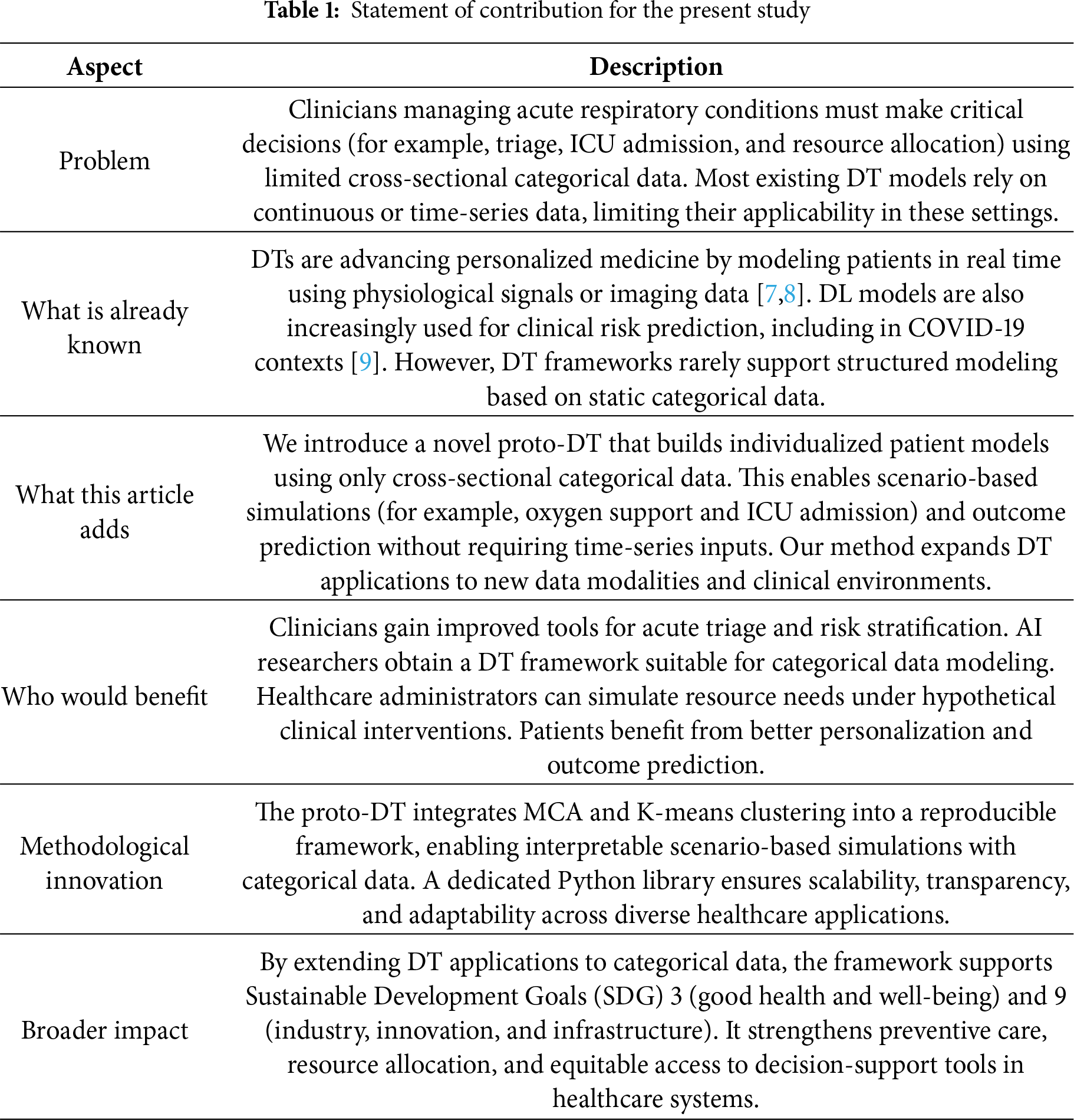
After detailing our contributions in Table 1, we now outline the clinical relevance and real-world support of these contributions. The proto-DT framework proposed in this study responds to a recognized gap in healthcare practice, that is, the difficulty of capturing rapid changes in patient conditions using static cross-sectional data. Recent literature emphasizes that AI must evolve beyond predictive accuracy to provide transparency and adaptability in real-world clinical contexts. The integration of machine learning and AI into clinical medicine has accelerated dramatically, but it also stresses that interpretability and methodological rigor are prerequisites for clinical adoption [22]. This observation aligns with our methodology, which leverages categorical data to simulate evolving patient scenarios, thereby offering clinicians a tool that bridges the divide between static models and dynamic patient trajectories.

Explainability has emerged as a critical requirement for trust and accountability in healthcare and other fields [23]. Through a systematic review [24], it was demonstrated that explainable AI methods such as Shapley additive explanations and local interpretable model-agnostic explanations are increasingly applied in disease prediction. However, current models often rely on limited datasets and single data modalities [24]. Similarly, the growth of research on interpretable AI in medicine was documented in [25], underscoring the necessity of balancing performance with transparency. This reinforces the relevance of our proto-DT, prioritizing interpretability by enabling scenario-based simulations that clinicians can directly inspect and reason about.

Parallel advances in DT technology further illustrate the importance of real-time monitoring and adaptive modeling. A DT framework was proposed in [26], which integrates real-time sensor data with historical records, achieving high accuracy in patient monitoring but also revealing challenges in scalability and cybersecurity. Complementing this, a meta-review of healthcare DTs was provided in [27], identifying key barriers such as data quality, ethical concerns, and clinical validation. These advancements highlight that, while DTs hold transformative potential, their adoption remains constrained by technical and organizational limitations. Our proto-DT contributes to this evolving field by offering a scalable and interpretable methodology that can be implemented even with modest categorical datasets.

Note that AI must adapt to dynamic patient trajectories to improve outcomes and equity in healthcare delivery [28], indicating that deployment requires. technical innovation and clinician training, regulatory oversight, as well as ethical safeguards. Thus, our framework shows how single-point categorical data can be transformed into actionable information that simulates aspects of a DT. By aligning methodological innovation with clinical needs, the proto-DT methodology strengthens preventive care, supports resource allocation, and enhances transparency in patient risk assessment. This integration of explainability and adaptability shows the advancement of our proposal, positioning the contribution as a reliable and clinically meaningful AI solution.

The remainder of this article is structured as follows. Section 3 describes data, their preprocessing, and classification models, that is, a deep neural network (DNN), logistic regression (LR), random forest (RF), and extreme gradient boosting (XGBoost). In Section 4, we present the results and scenario-based simulations. In Section 5, the proto-DT model is expanded through simulation-based studies and the application of multiple correspondence analysis (MCA) and K-means clustering. Section 6 presents our main findings and their clinical and operational implications, while Section 7 outlines the conclusions of the study together with its limitations. Appendices A and B contain the Python code and supporting material.

2  Mathematical and Conceptual Background

2.1 Proto-Digital Twin Concept

Traditional DT systems in healthcare typically rely on continuous or longitudinal data streams, enabling near real-time modeling of disease progression, intervention effects, and patient trajectories [16,17,21]. Such systems dynamically update a virtual representation of the patient to mirror ongoing clinical changes, often requiring high-frequency inputs from sensors, electronic health records, or wearable devices [29]. However, many healthcare environments—especially large-scale observational settings—lack access to these data streams and instead rely on cross-sectional snapshots of patient status, stating a limitation.

To address this limitation, we propose a proto-DT framework that uses purely cross-sectional data to approximate certain functionalities of a traditional DT. Although this framework does not provide a fully dynamic model of patient evolution, it does enable scenario-based analyses of hypothetical interventions. Specifically, we employ our trained DNN to simulate how changes in key variables, such as ICU admission, vaccination status, or oxygen support, might alter a patient’s predicted risk of mortality. The workflow proceeds with the following analyses:

•   Baseline profile—A patient’s one-hot-encoded feature vector is copied as the baseline scenario.

•   Intervention simulation—Selected variables (for example, ICU admission or oxygen support type) are modified to represent a possible clinical intervention or status change.

•   Outcome recalculation—The same predictive model recalculates mortality probability under these revised features, facilitating a before-and-after comparison.

These analyses generate what-if scenarios at the individual-patient level, without requiring longitudinal data. For instance, one may ask whether earlier ICU admission or additional vaccination doses could reduce the patient’s predicted mortality risk. While these questions remain purely hypothetical in a cross-sectional context, they state how the model weighs critical risk factors and identify which variables exert the strongest effect. From a methodological standpoint, they are similar to counterfactual or scenario-based analyses in machine learning, which systematically alter input variables to examine model sensitivity and feature importance [30].

Fig. 1 illustrates the proto-DT workflow. The process begins by encoding a patient’s categorical features to form a baseline profile. Next, a chosen intervention (for example, changing the “ICU” flag from “No” to “Yes”) is applied, creating a hypothetical scenario. The DNN subsequently recalculates the mortality probability under these modified conditions, enabling a direct comparison of baseline and intervention outcomes. Crucially, this process does not require temporal information as it operates on a single cross-sectional input while still yielding insights into how particular risk factors might affect model predictions. It is essential to note that the simulations do not establish causation. The proto-DT framework provides a preliminary vision to examine how specific clinical measures, if implemented hypothetically, could alter predicted mortality. A fully realized DT would incorporate temporal data, dynamic updates of patient parameters, and more advanced causal inference methods. Nonetheless, for contexts lacking frequent data acquisition, the proto-DT concept can give insights into outcomes of major clinical interventions and serve as a proxy toward a more comprehensive real-time DT system.

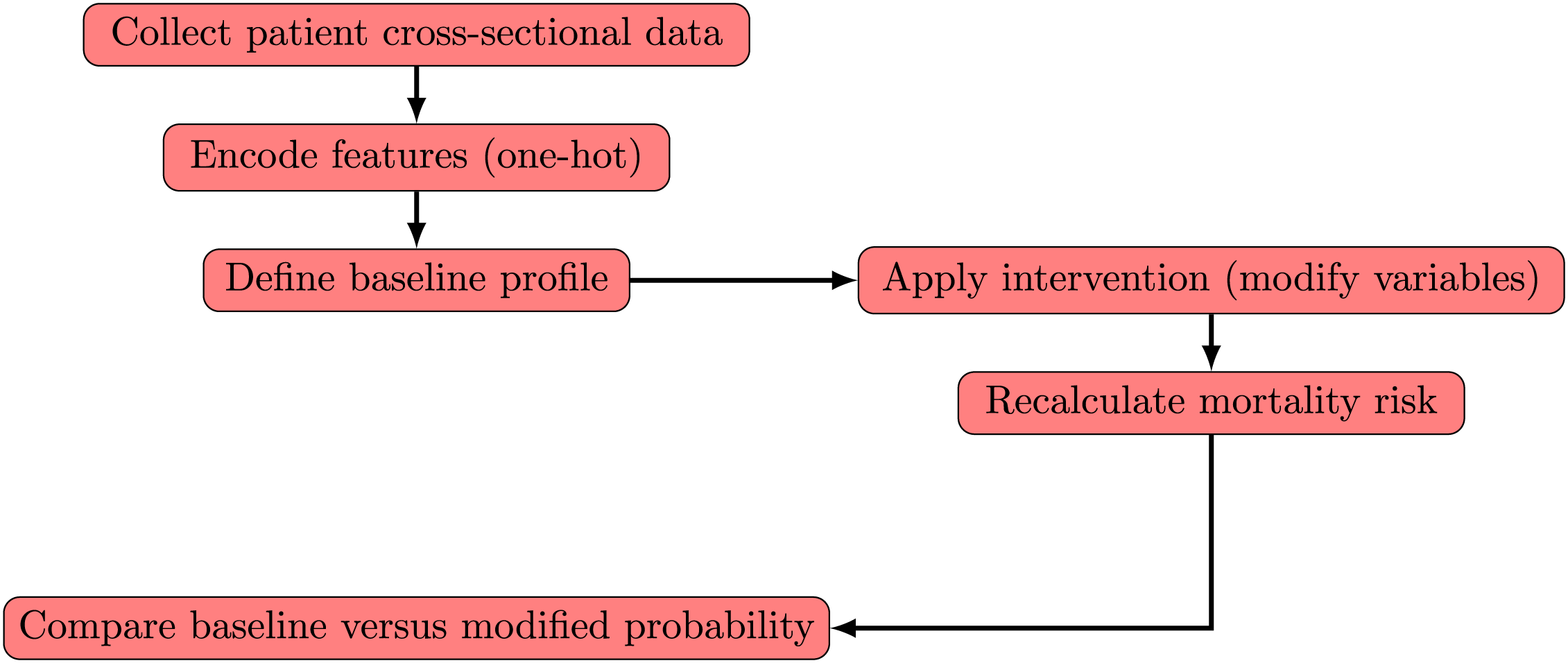
Figure 1: Workflow of proto-DT framework with patient cross-sectional data and hypothetical interventions

2.2 Mathematical Background for Proto-Digital Twins

Traditional DT frameworks typically rely on longitudinal or sensor-based data to update a virtual patient representation over time. In contrast, our proto-DT operates in a purely cross-sectional setting, that is, each patient is described by a one-hot-encoded categorical vector x0∈{0,1}p, and no temporal evolution is observed. Consequently, the mathematical formulation used in dynamic DTs (state–space models, stochastic process noise, and survival trajectories) must be adapted to the static nature of the available data as follows.

First, we introduce a single-step intervention operator. To simulate hypothetical interventions, we define a deterministic modification operator as

x1=f(x0,u0,θ),(1)

where u0∈𝒰 represents an admissible intervention (for example, switching “ICU = No” to “ICU = Yes”). Note that 𝒰 shown in (1) denotes the set of admissible interventions, and 𝒳 denotes the space of feasible categorical profiles to which both x0 and x1 must belong. In cross-sectional data, f does not represent a physiological process over time, but instead performs controlled edits on categorical indicators according to the chosen intervention. The vector θ denotes the collection of model parameters estimated from the data. These parameters summarize the information learned during training and remain fixed during all intervention scenarios.

Second, we state the predictive model. The previously defined parameter vector θ characterizes the trained classifier, which induces the mapping formulated as

y1=g(x1;θ),(2)

returning the predicted mortality probability under the modified profile. The function g stated in (2) represents the learned predictive mechanism (such as DNN, LR, RF, or XGBoost), and it operates on the counterfactual covariate vector x1.

Note that no temporal sequence (xt) is generated; instead, (x0,x1) denote the baseline and intervention-induced configurations evaluated by the model.

Third, we discuss the ranking of interventions via a single-step cost. Although traditional DT control problems use multistep objectives, for cross-sectional data we adopt the single-step formulation given by

J(u0)=‖x1−xtarget‖Q2+λ‖u0‖R2,(3)

where Q and R are weighting matrices. The scalar λ>0 presented in (3) controls the relative penalization of intervention magnitude, where larger values discourage substantial or clinically unlikely modifications, while smaller values allow more flexibility. The first term penalizes deviation from the desired clinical profile, and the second term penalizes the size of the applied modification. This single-step cost serves to rank candidate interventions rather than to optimize a temporal trajectory.

Lastly, we refer to federated learning. Here, θ is the same parameter vector defined above, now updated through federated aggregation. In multi-institutional settings, parameter estimation follows the objective stated as

minθ{∑i=1IwiLi(θ)},(4)

where Li is the local loss at site i, wi≥0 are aggregation weights, and θ(r+1)=∑i=1Iwiθi(r) are local model updates, all of them defined in (4). Only aggregated summaries are shared, preserving privacy.

2.3 Multiple Correspondence Analysis

MCA is used to study relationships among categorical variables by embedding them into a continuous low-dimensional space. Let X∈{0,1}n×p denote the complete disjunctive matrix encoding n individuals and p categories derived from m categorical variables. Each row corresponds to an individual, and each column to a category indicator. The Burt matrix is defined as B=(1/n)X⊤X, whose diagonal blocks contain category frequencies and off-diagonal blocks encode pairwise associations.

MCA is performed by decomposing the standardized matrix given ny

Z=Dr−1/2((1/n)X−rc⊤)Dc−1/2,(5)

where r and c established in (5) are the row and column marginal proportions, and Dr=diag(r) and Dc=diag(c) are diagonal weighting matrices.

The singular value decomposition Z=UΣV⊤ yields the principal coordinates F=Dr−1/2UΣ and G=Dc−1/2VΣ, which represent individuals and categories, respectively. Here, U and V denote the left and right singular vectors.

Each eigenvalue λℓ in Σ2 measures the proportion of total association explained by the ℓ-th component. Plotting the category coordinates G enables visualization of latent structures and relationships among patient attributes.

Within our proto-DT framework, MCA provides a continuous embedding of categorical patient profiles that supports dimensionality reduction, visualization, and subsequent integration with simulation-based analyses.

2.4 K-Means Clustering

K-means is a partitioning algorithm that groups n observations into K clusters by minimizing within-cluster variance. Let {x1,…,xn} denote the set of patient profiles embedded into a continuous space (for example, using MCA), where each xi∈Rd and d is the dimension of the embedding. The corresponding objective function is defined as

𝒞=∑i=1n∑k=1Krik‖xi−μk‖2,(6)

where rik∈{0,1} presented in (6) is the assignment indicator (equal to 1 if point i is assigned to cluster k and 0 otherwise), and μk∈Rd is the centroid of cluster k. The centroids are updated iteratively according to μk=∑i=1nrikxi/∑i=1nrik, which corresponds to the mean of all points assigned to that cluster.

The K-means algorithm alternates between the two steps following:

•   Assignment step —Assign each to the nearest centroid using

rik={1,if k=arg⁡minj{‖xi−μj‖2};0,otherwise.

•   Update step —Recompute the centroids using the mean of their assigned points as μk=∑i=1nrikxi/∑i=1nrik.

Convergence is reached when cluster assignments stabilize or when the decrease in 𝒞 falls below a predefined tolerance. The distance metric ‖⋅‖2 is the squared Euclidean norm, ensuring that clusters minimize within-group variance.

The choice of K can be guided by indices such as the silhouette coefficient or the elbow method, which evaluate the trade-off between within-cluster compactness and between-cluster separation. In our proto-DT framework, K-means provides an interpretable grouping of categorical patient profiles, complementing MCA embeddings and supporting downstream simulation and outcome analysis.

3  Methodology

3.1 Data Source and Preprocessing

This study relies on data reported between January and December 2022 through the Brazilian Unified Health System. After removing a small number of duplicated or invalid entries during an initial quality check, the definitive dataset included 415,711 individuals with severe acute respiratory infection (SARI). The dataset is publicly available from the Brazilian Ministry of Health [31] platform. These records encompass both confirmed and suspected COVID-19 cases, as well as non-COVID-19 instances, providing coverage across the entire Brazilian territory.

The dataset originates from the national surveillance system for SARI, maintained by the Brazilian Ministry of Health. This platform was initially created to monitor influenza AH1N1 in 2009 and expanded in 2020 to include COVID-19 surveillance. Reporting of SARI cases is mandatory for all healthcare facilities, both public and private, ensuring comprehensive coverage across the country. From this system, fourteen demographic and clinical variables were selected due to their direct relevance to SARI hospitalizations and outcomes. These variables capture comorbidities, vaccination status, respiratory symptoms, ICU admission, oxygen support, and patient outcomes, providing a categorical representation that is particularly suitable for modeling with our proto-DT framework.

In a first step, we removed a small number of duplicated or invalid entries during an initial quality check (duplicated patient records or cases with incomplete data that could compromise the dataset being internally coherent, complete, and usable, as well as affect the validity of the analysis and the reliability of the results). According to official curation procedures, the database had already minimized missing values in the main variables of interest, so only a very small number of records required removal during our initial quality check. This step ensured that the dataset retained uniformity in key attributes and was suitable for our classification methods.

To provide greater clarity regarding the dataset used in this study, Table 2 summarizes the fourteen categorical variables included in the definitive analysis. Each variable was selected based on its clinical relevance to severe respiratory infections and its availability in the surveillance records. The table also illustrates how these variables were encoded, ensuring transparency in the modeling process and facilitating reproducibility of the proposed proto-DT framework.

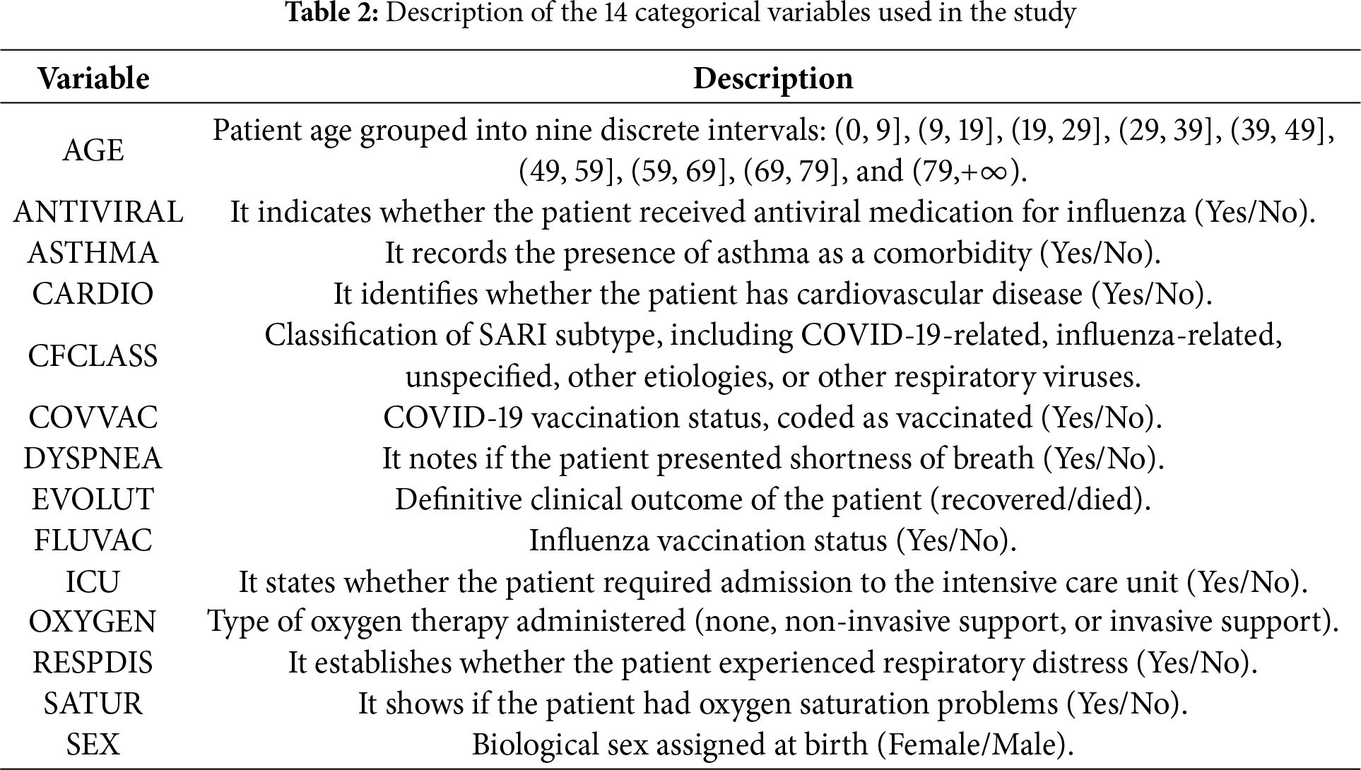
As mentioned, the definitive dataset comprised 415,711 observations after the initial quality check and included 14 categorical variables capturing key clinical and demographic factors. These variables encompassed patient age (grouped into intervals), presence of asthma and cardiovascular disease, vaccination status for COVID-19 and influenza, use of antiviral medication, reported symptoms (shortness of breath, respiratory distress, and oxygen saturation levels), type of oxygen support received, admission to ICU, biological sex, and patient outcomes (recovered or died). Additionally, a variable indicating whether the case was related to COVID-19 or not was included.

Most patients (78.3%) recovered, while 21.7% succumbed to their conditions, highlighting the imbalanced nature of the dataset. COVID-related cases accounted for 45.2% of the records. Regarding age distribution, the majority were children aged 0 to 9 years (26.0%), followed by individuals aged 79 and above (20.9%) and those aged 69 to 79 years (15.7%). The dataset included a nearly equal distribution of sexes, with 49.2% female and 50.8% male patients. Among all patients, 26.1% required admission to the ICU, and oxygen support was predominantly non-invasive (61.1%), with invasive support used in 11.8% of cases. Also, 61.5% of the patients received at least one dose of the COVID-19 vaccine. Among the patients who succumbed to their conditions (21.7%), 52.7% were male and 47.3% female. Mortality rates were highest among individuals aged 79 and above (38.2%), followed by those aged 69 to 79 years (24.1%) and 59 to 69 years (16.7%); 2.36% of the deaths occurred in children aged 0 to 9 years. In intensive care, 48.1% of the deceased patients required admission to the ICU. Oxygen support was mainly non-invasive (53.8%), while 35.9% received invasive support, and 77.8% received at least one dose of the COVID-19 vaccine.

The suitability of the fourteen categorical variables employed in our proto-DT framework is supported by prior studies that have consistently identified demographic and clinical factors as relevant predictors of mortality in severe respiratory infections. Comorbidities and severity scores, such as SOFA and APACHE, were strongly associated with poor prognosis in critically ill COVID-19 patients [32], highlighting the importance of age and baseline health conditions. Similarly, advanced age, comorbidities, and oxygen saturation levels were shown [33] as independent predictors of in-hospital mortality among older patients, reinforcing the clinical relevance of variables such as age, comorbidities, and respiratory status.

Extending this evidence, a systematic review of prognostic models [34] confirmed that age, comorbidities, ICU admission, and oxygen support are among the most frequently used predictors of adverse outcomes, despite methodological heterogeneity across studies. More recently, complex interactions between age, cardiac conditions, and pulmonary comorbidities were identified [35] and determined mortality risk, further validating the inclusion of comorbidity-related variables in predictive frameworks. Also, the predictive value of simple clinical parameters, such as respiratory rate and oxygen saturation in patients aged 65 years and older, was highlighted [36], supporting the use of categorical respiratory variables in large-scale epidemiological surveillance datasets.

Nonetheless, it is important to acknowledge a limitation of our study, since our dataset does not include vital signs, laboratory values, or severity scores (for example, SOFA and APACHE scores, or sepsis/shock status), which are commonly employed in ICU-based mortality models [32,33]. This limitation reflects the epidemiological surveillance dataset nature of the database, which prioritizes standardized categorical reporting across healthcare facilities nationwide. Nevertheless, the large sample size and nationwide coverage provide a unique opportunity to model mortality risk at the population level, complementing rather than replacing ICU-based prognostic tools.

3.2 Class Imbalance and Rationale for Cost-Sensitive Weighting

The dataset’s imbalanced nature, with recoveries outnumbering mortality cases, needed to address this imbalance [37]. Oversampling, such as synthetic minority over-sampling [38], and undersampling methods can distort the original data distribution, particularly in large datasets with high feature cardinality. To avoid this distortion, we adopted cost-sensitive weighting, increasing the training penalty for misclassifying minority-class examples. In the DNN, LR, and RF models, we applied an internal weighting scheme, while in XGBoost, we set a parameter according to the ratio of negative to positive cases [39]. Preliminary experiments indicated that these cost-sensitive methods provided adequate recall for the mortality class, without a significant increase in false positives (FPs) or compromising model interpretability. Complementary exploratory experiments considered alternative oversampling procedures and more advanced methods for categorical features, which may be beneficial in scenarios involving small sample sizes or more extreme imbalance.

3.3 Train-Test Split, Cross-Validation, Models, Implementation, and Evaluation

We divided the dataset into training (80%) and test (20%) partitions in a stratified manner, preserving the proportion of mortality and non-mortality outcomes in each subset. On the training portion, we applied a five-fold cross-validation scheme to optimize hyperparameters and reduce overfitting. In this scheme, each record contributes to both model training and validation in different folds, with better results. Then, the best-performing configuration is retrained on the entire training set and evaluated on the held-out test subset to gauge real-world generalization and provide an unbiased assessment. Fig. 2 presents a scheme of the modeling from data splitting to definitive evaluation.

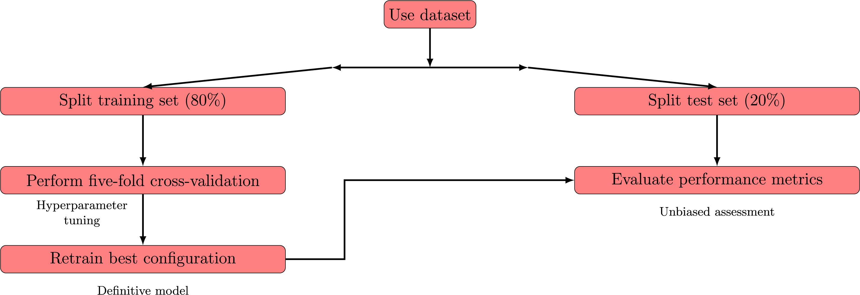
Figure 2: Schematic representation of the process

We consider four classification models: DNN, LR, RF, and XGBoost. All models were developed in a high-level programming environment that employed established open-source libraries, without relying on specific software-level function calls in the methodological description. Below, we summarize each model structure and hyperparameters, drawing on standard references in the literature.

A traditional LR model [40] was used with a cost-sensitive objective that imposed heavier penalties on minority-class misclassifications. The regularization strength and cost parameters were tuned via preliminary cross-validation to maintain a balance between overfitting and underfitting.

For the RF model [41], we likewise applied a scheme that upweighted minority-class samples during each bootstrap iteration. Core hyperparameters, including the number of trees and maximum tree depth, were determined through a systematic grid-based search [42], with the aim of maximizing recall for the mortality class while preserving high accuracy overall.

A tree-based XGBoost model, adapted from [39], was also tested. Its cost-sensitive weighting was set proportionally to the ratio of negative to positive samples, and cross-validation was employed to fine-tune both the learning rate and maximum tree depth, ensuring stable convergence. Lastly, we implemented a feed-forward DNN model with two hidden layers of 128 and 64 units, respectively, each followed by a 50% dropout [43] to mitigate overfitting. The output layer consisted of a single neuron with a logistic activation [44], supporting binary classification. Model training used an adaptive moment estimation method [45], with a mini-batch size of 256 and up to 100 epochs. A cost-sensitive loss function increased the penalty for minority-class errors, and a validation subset was reserved to monitor and mitigate overfitting.

After identifying the optimal hyperparameters for each model, we retrained the definitive versions on the entire training set. Then, an independent test set was used to evaluate generalization performance and to compare all four models on the same footing. A comprehensive assessment of classification models in healthcare usually requires several metrics, each highlighting a different aspect of predictive performance [30,40]. The elements of Table 3 are used to measure performance. Based on Table 3, the performance metrics computed on the test sets are presented in Table 4.

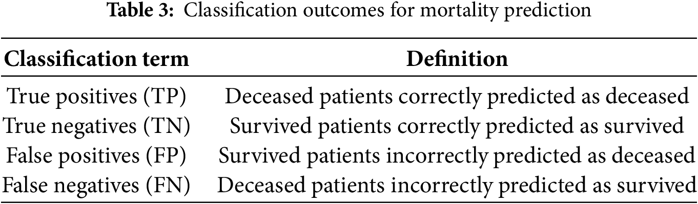
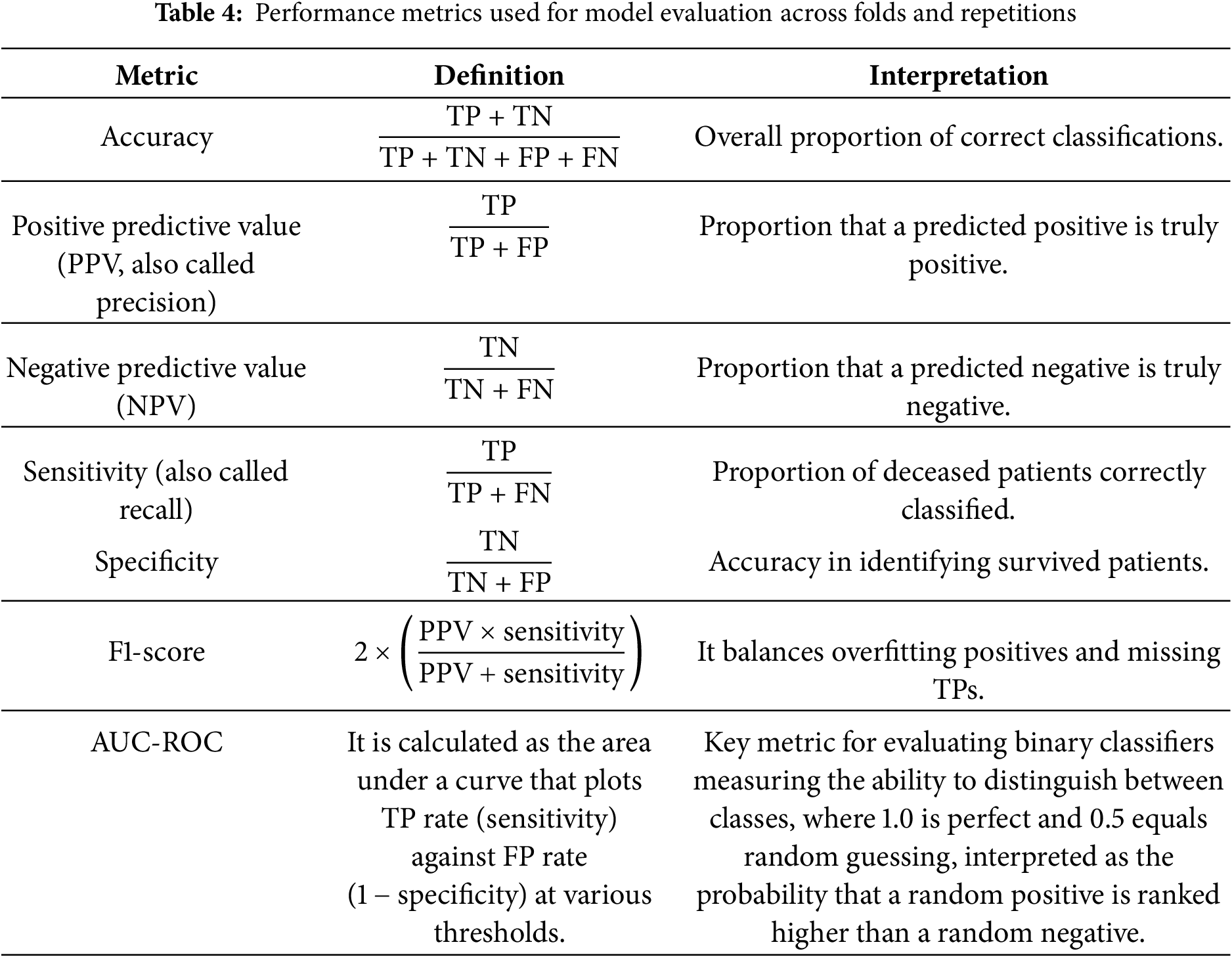
All these metrics simultaneously provide a comprehensive view of the model’s performance, quantifying the trade-off between FN—critical to avoid missed severe cases—and FP—which may strain limited resources. Although high recall is vital for identifying critical cases, it may need to be balanced with precision when resources are constrained [37,38]. In addition, strong results on these metrics do not guarantee accurate probability estimates, which is a key consideration if clinicians rely on predicted risk scores for decision-making [30]. Hence, additional evaluations such as calibration curves or Brier scores may be required to confirm alignment between predicted and actual outcomes.

All experiments were conducted in a stable computing environment (32 GB RAM) using open-source libraries and systematic hyperparameter tuning, as mentioned. These performance indicators are influenced by choices in data preprocessing, feature engineering, and model configuration [40]. Consequently, although accuracy, precision, recall, F1-score, and AUC-ROC are valuable proxies for clinical utility, further validation through external cohorts or prospective trials remains essential to establish each model’s reliability in real-world healthcare settings.

3.4 Overview of the Methodological Workflow

The methodological workflow of the proto-DT framework is summarized in this subsection. The process begins with the acquisition of surveillance data from the Brazilian Ministry of Health, followed by an initial quality check to remove duplicated or invalid records. After preprocessing, the definitive dataset comprised 415,711 patients described by 14 categorical variables capturing demographic and clinical information.

To address the imbalance between recovered and deceased patients, cost-sensitive weighting was applied during model training. Then, the dataset was divided into stratified training and test subsets, with hyperparameters optimized through five-fold cross-validation. Four classification models were implemented—DNN, LR, RF, and XGBoost—and evaluated using accuracy, precision, recall, F1-score, and AUC-ROC, complemented by calibration analyses. This workflow ensures that the framework provides interpretable and balanced results, while highlighting the need for external validation in real-world healthcare settings.

The methodological framework is represented in two complementary flowcharts. The first diagram (Fig. 3) provides an overview of the proto-DT framework, from data collection and preprocessing to model training, evaluation, and reporting. The second diagram (Fig. 2) focuses specifically on the modeling and evaluation sub-process, detailing how the dataset is split, hyperparameters are tuned, and definitive performance is assessed. Both figures illustrate both the global workflow and the internal mechanics of the modeling stage, ensuring clarity and coherence in the presentation of the methodology.

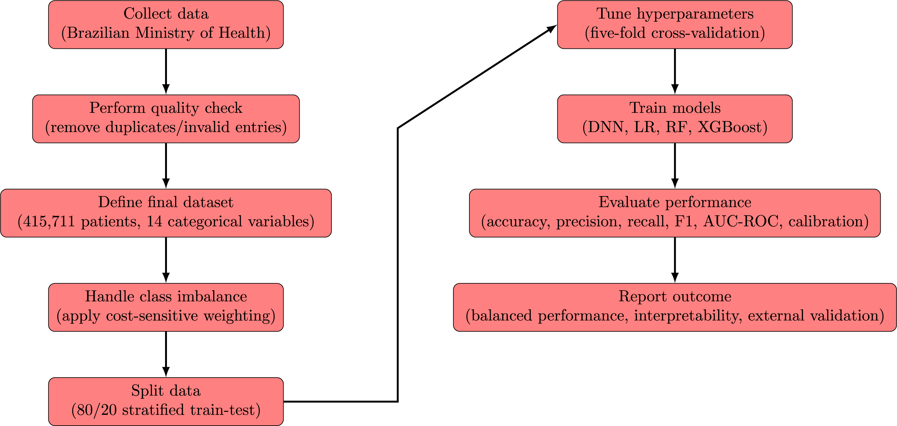
Figure 3: Flowchart of the proto-DT framework step by step from data collection to evaluation

4  Results

4.1 Overall Performance of the Classification Models

We trained four machine learning models (DNN, LR, RF, and XGBoost) on the stratified dataset. Table 5 summarizes their performance on the test set.

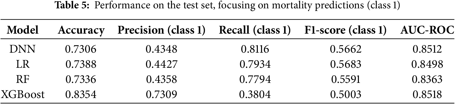
From Table 5, note that the LR model obtained an AUC-ROC of 0.8498, indicating reasonable discrimination between survivors and non-survivors. Its recall for the mortality class was 0.79, suggesting strong sensitivity in detecting high-risk patients. However, the precision of 0.44 indicates that many of these positive classifications may be false alarms, which can lead to added resource usage in a clinical context. Also from Table 5, the RF model showed patterns similar to LR, with a recall of 0.78, an accuracy of 0.73, and an AUC-ROC of 0.836. Although its overall AUC-ROC was somewhat lower, it still demonstrated adequate sensitivity toward mortality cases. This result partly reflects the benefit of cost-sensitive weighting, which places additional emphasis on correctly identifying minority-class observations [37,38]. Nonetheless, precision remained close to 0.44, mirroring the trade-off observed in the LR model. Similarly, from Table 5, the XGBoost model achieved the highest overall accuracy (0.84) and the highest AUC-ROC (0.8518). However, its recall for the mortality class was 0.38, indicating that many severe cases may go undetected if the default probability threshold of 0.5 is retained [39].

In a clinical setting, this model would produce few FPs but could fail to flag some critically ill patients. The DNN model reached an AUC-ROC of 0.851, comparable to XGBoost, and attained the highest recall (0.81) for the mortality class. The DNN model rarely misses a fatal case, though its precision of 0.43 suggests more FPs. This trade-off may be acceptable where the priority is to identify every possible high-risk patient, recognizing that additional screening may be required for those flagged incorrectly. The results presented in Table 5 are shown in Figs. 4 and 5.

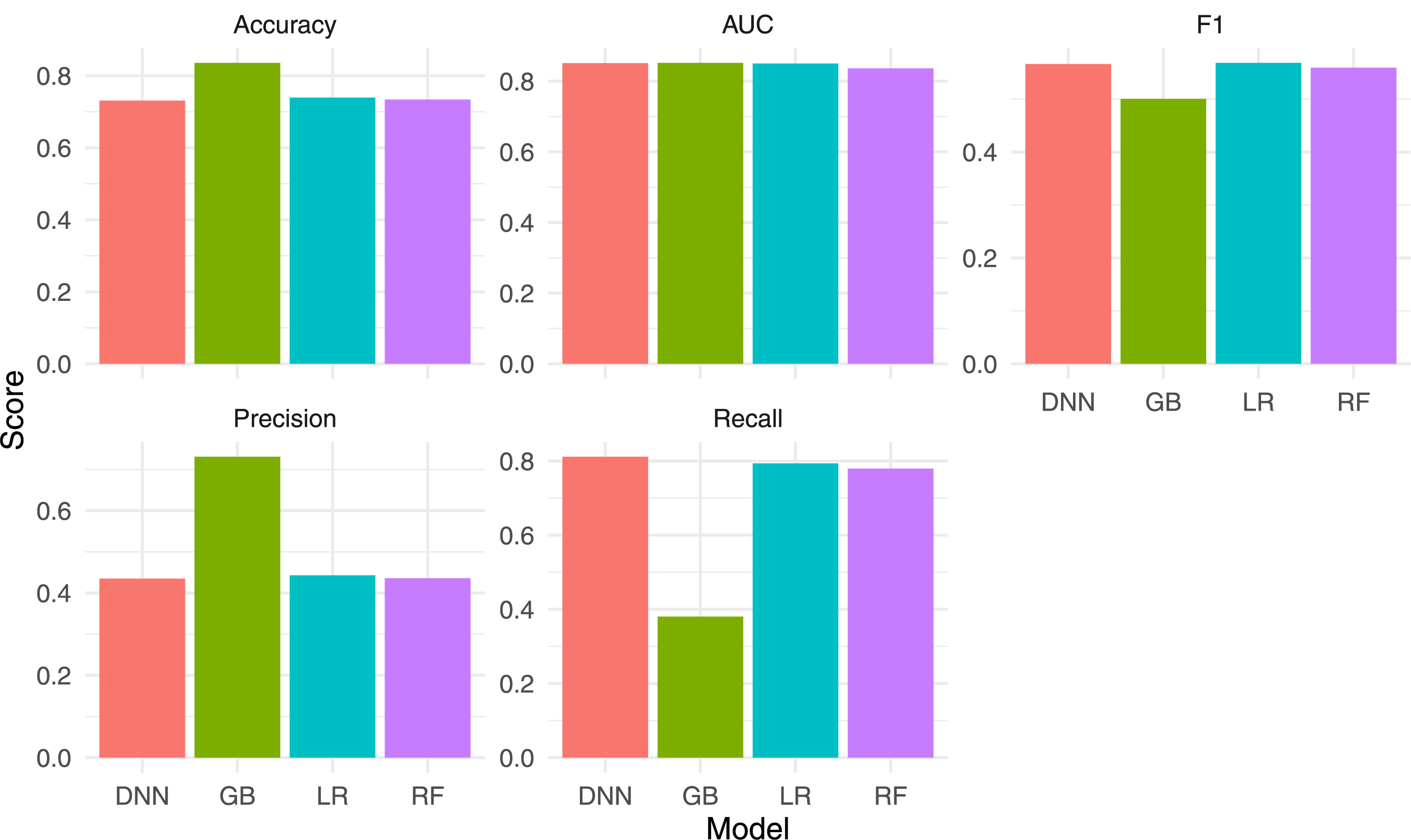
Figure 4: Bar chart comparing the main performance metrics for the four models

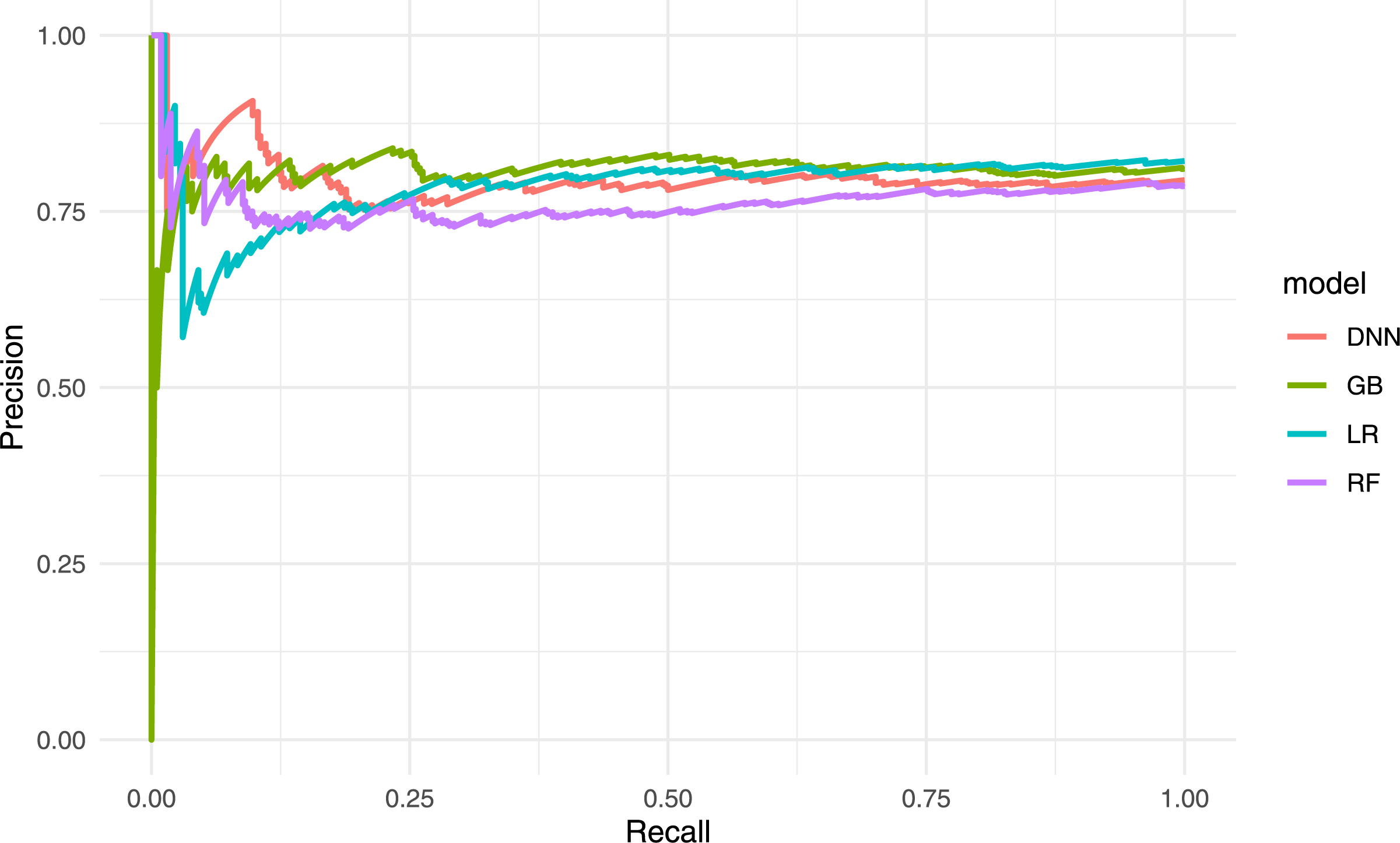
Figure 5: Precision–recall curves for the four models

4.2 Confusion Matrices and Error Analysis

To explore the patterns of misclassification in detail, confusion matrices were examined (not shown here for brevity) to distinguish FPs from FNs. The LR and DNN models placed greater emphasis on recall, capturing most fatal cases but generating more FPs, whereas XGBoost produced fewer false alarms but overlooked a larger fraction of high-risk patients.

The RF and LR models presented similar trade-offs, likely due to cost-sensitive weighting and the largely categorical nature of the dataset, which allows LR to capture principal effects through one-hot encoding. If deeper interactions are limited, RF does not gain much beyond those main effects. Hence, both models maintain reasonable recall with a precision of around 0.44.

The DNN model achieved the highest recall among all classifiers but with lower precision, implying that it flagged more patients as high risk than necessary. By contrast, the XGBoost model had the highest accuracy and AUC-ROC but reduced sensitivity to mortality, potentially missing individuals needing urgent care [39]. In clinical practice, threshold tuning or cost adjustments could mitigate this by lowering the decision boundary, though that would increase the false-positive rate.

In summary, each model exhibits distinct advantages and limitations. The XGBoost and DNN models excel in accuracy and recall, respectively, while the LR and RF models occupy intermediate ground with a balanced trade-off between the two. The best choice depends on how costs and benefits are weighed, particularly when missing a critically ill patient may have a higher clinical cost than temporarily allocating resources to a low-risk individual.

4.3 Scenario-Based Proto-Digital Twin Analysis

To illustrate how a cross-sectional proto-DT can provide preliminary insights into patient outcomes, we conducted a series of hypothetical “what-if” interventions. Table 6 lists example modifications, each of which alters one key input variable in a patient’s encoded profile (such as changing vaccination status or ICU admission). Then, the trained model is used to re-evaluate mortality risk under these altered conditions, so indicating how sensitive the model is to each variable.

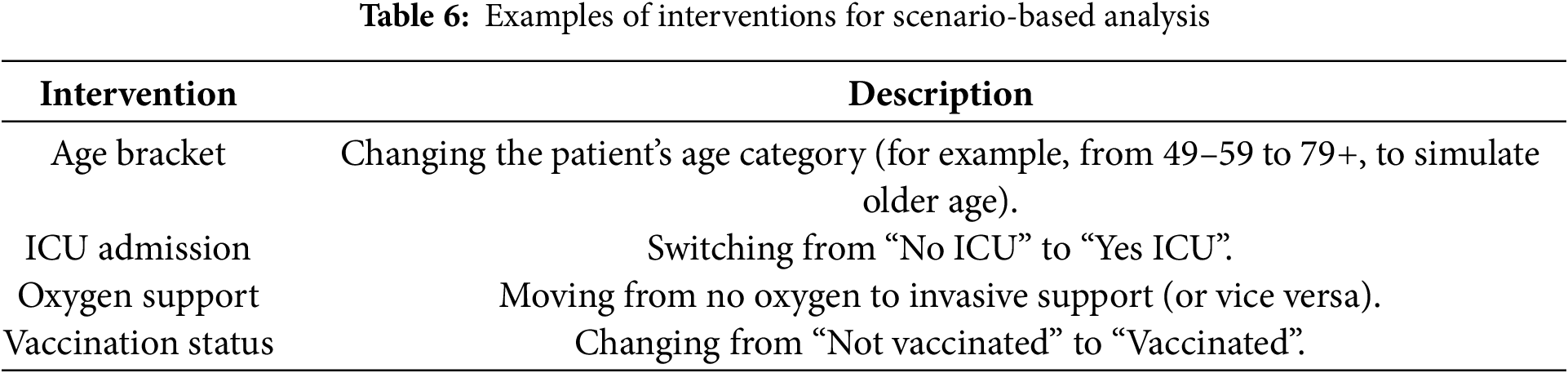
Fig. 6 conceptualizes our analysis. A baseline patient profile (encoded in one-hot format) is copied. Select variables are modified to reflect a hypothetical clinical scenario. Then, the model recalculates the mortality probability, allowing direct comparison between baseline and modified risk estimates. Although these scenario tests rely on a single cross-sectional snapshot, they provide model-based sensitivity analyses that highlight potential drivers of mortality within the dataset.

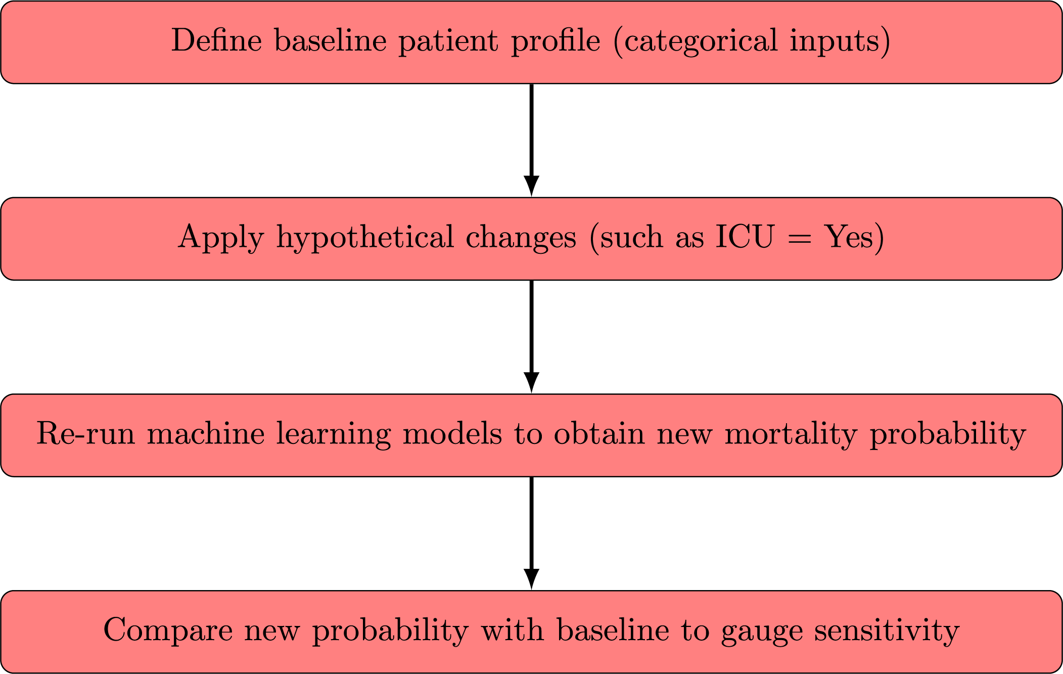
Figure 6: Flowchart of the scenario-based proto-DT analysis with cross-sectional data

Table 7 presents an illustration of a patient aged 49 to 59 years, not admitted to the ICU, vaccinated, and not receiving invasive oxygen therapy. The second column of the table shows the predicted mortality probabilities estimated by each model for this baseline profile. The subsequent columns display the predicted probabilities under alternative scenarios in which a single condition is modified at a time, while all other patient characteristics remain fixed. The values reported in this table allow for a direct assessment of how incremental changes in clinically relevant factors influence predicted risk and illustrate the model’s ability to respond sensitively and coherently to realistic variations in a patient’s condition. These values highlight how our proto-DT framework can support clinicians in understanding the potential impact of specific patient characteristics on mortality risk, thereby reinforcing its practical utility for decision-making.

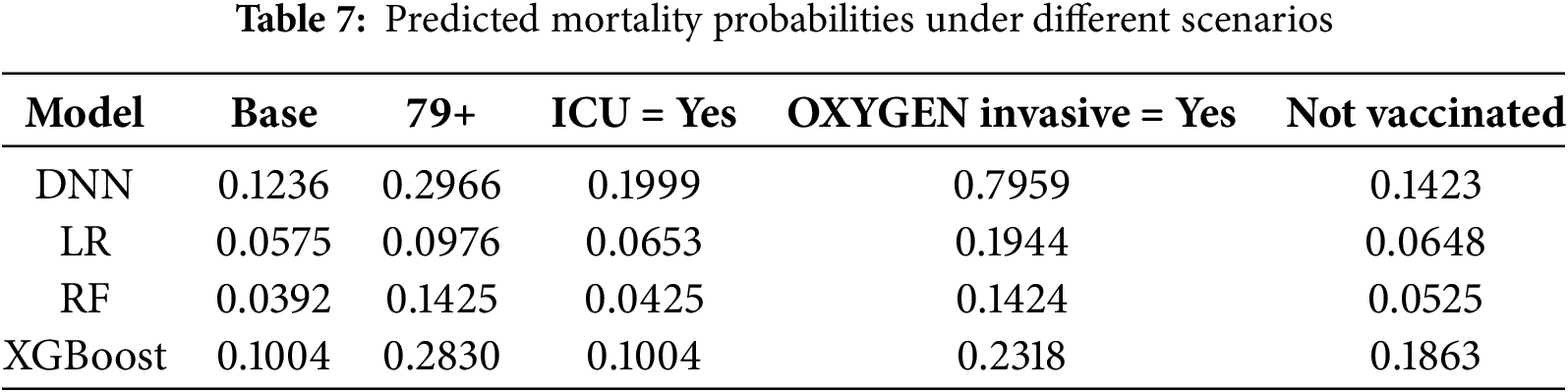
Several consistent patterns emerged from these preliminary scenario tests as follows:

•   Age bracket—Increasing a patient’s age category raised the predicted mortality probability, aligning with general clinical evidence that older adults are more vulnerable to severe complications from respiratory infections.

•   ICU admission—Switching from “No ICU” to “Yes ICU” typically elevated predicted mortality, reflecting that ICU admission correlates with higher illness severity in the underlying dataset (though not implying causation).

•   Oxygen support—Transitioning from no oxygen support to an invasive mode increased mortality risk predictions, suggesting that invasive oxygen therapy is associated with more severe disease states.

•   Vaccination—Changing an unvaccinated profile to “vaccinated” often lowered the predicted risk of death, consistent with broader epidemiological findings on vaccination benefits.

While these “what-if” outcomes do not establish causal links, they serve as a helpful exploratory tool to estimate how different clinical actions might shift mortality risks according to the model. In practice, modifying one or more features in the baseline profile and recalculating mortality risk allows clinicians or researchers to visualize the potential impact of specific interventions and refine their decision-making accordingly.

5  Extending the Proto-DT Framework through MCA and K-Means

5.1 Computational Framework

Appendix B outlines the functions implemented in the proposed Python library, which supports all computations and visualizations presented in this section.

After loading the data, the MCA model must be trained and the corresponding category plot for the 14 variables generated.

Fig. 7 shows the distribution of all categories following the application of MCA. The two components together account for 19.16% of the total variance. A K-means clustering analysis is conducted using the coordinates of the categories in the reduced-dimensional space. Prior to clustering, it is necessary to determine the optimal number of clusters for grouping the categories.

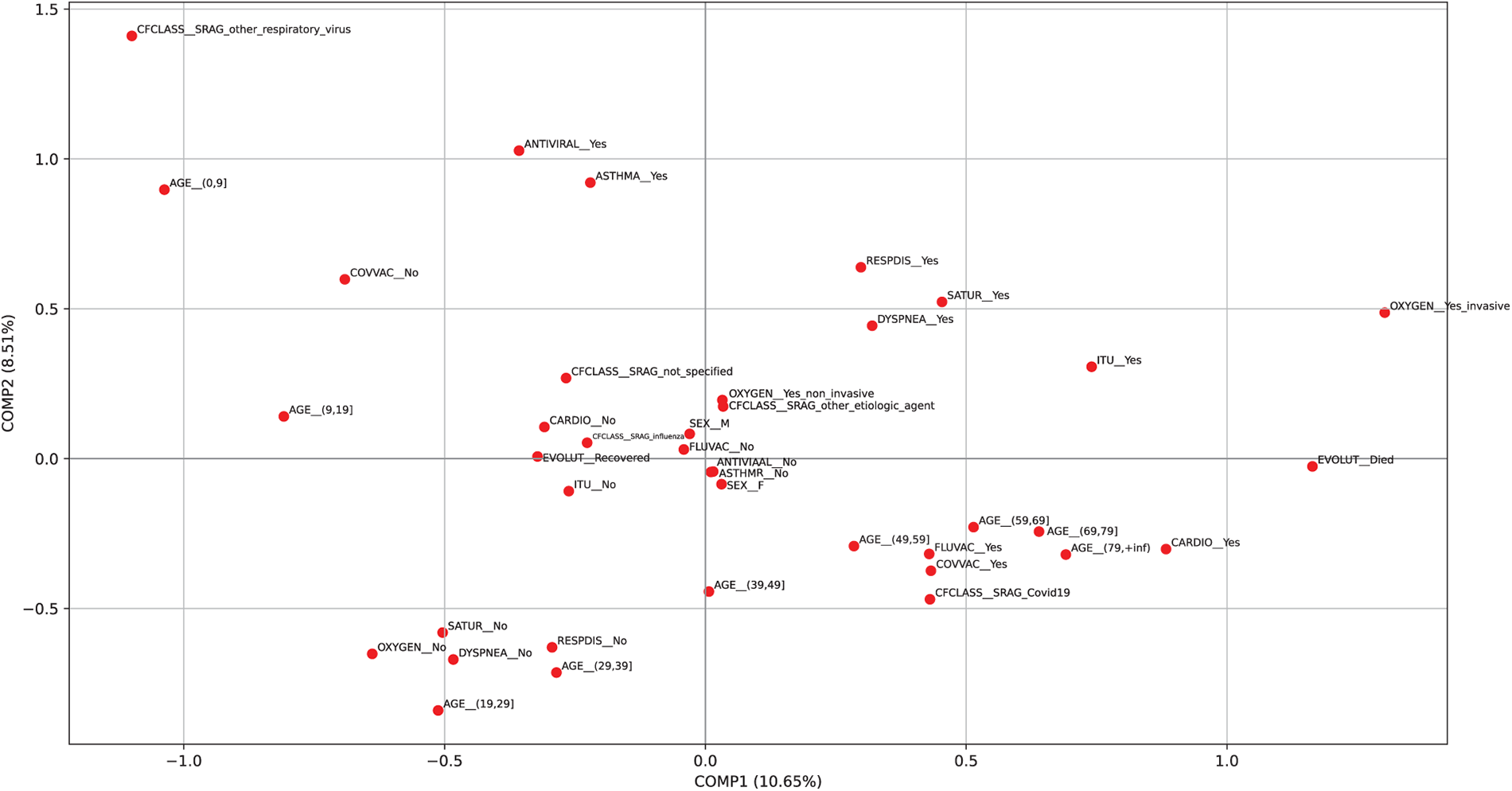
Figure 7: Plot of the categories from the MCA using the patient sample

5.2 MCA and K-Means Clustering Results on the Sample Data

In Table 8, the values of inertia and silhouette score are presented for varying numbers of clusters (ranging from k=2 to k=10), where k represents the total number of clusters considered. Fig. 8 presents a plot derived from the data in Table 8.

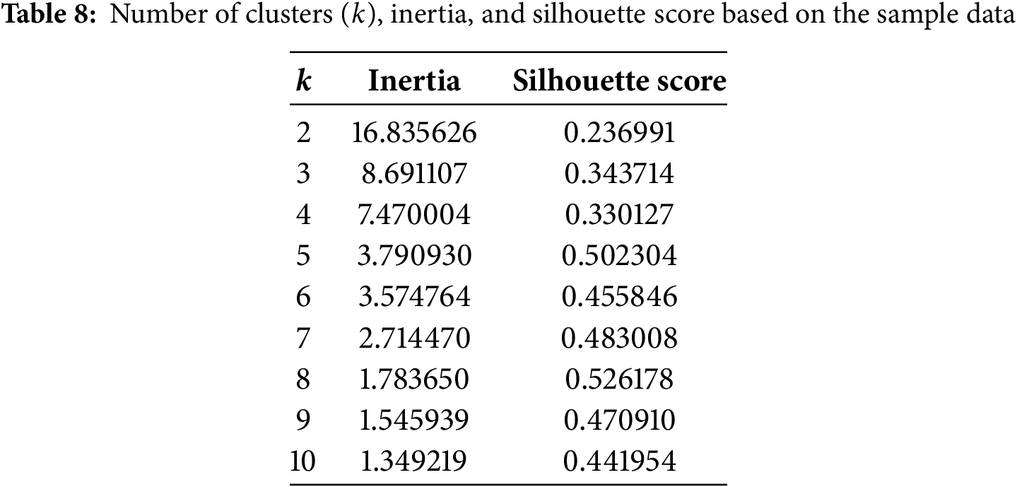
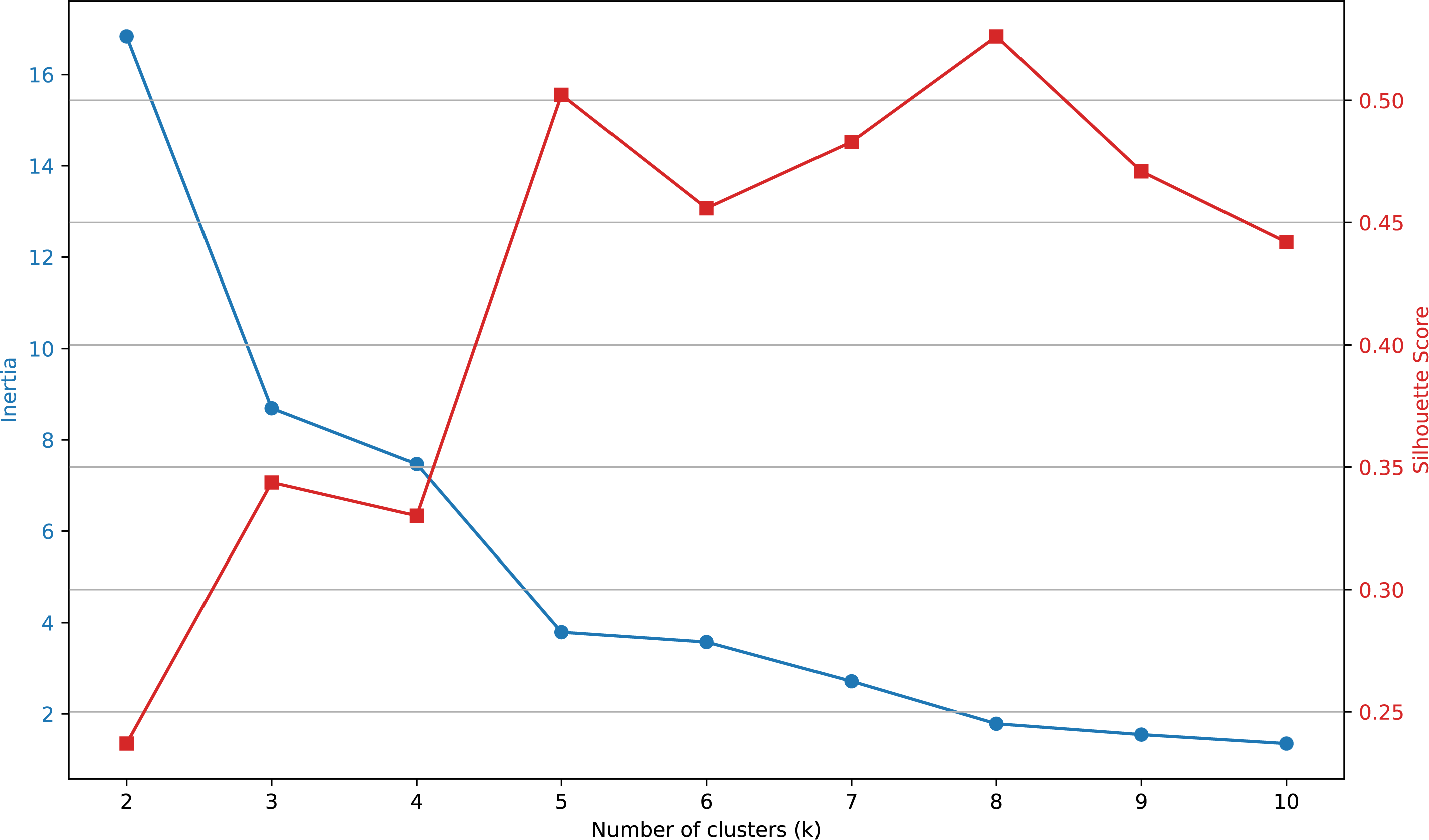
Figure 8: Elbow plot constructed using the values presented in Table 8

The results suggest that a suitable number of clusters for grouping the categories is k∗=5. Considering the joint analysis of inertia and the silhouette score, the choice of five clusters provides a suitable compromise between intra-cluster compactness and inter-cluster separation, achieving high-quality clustering without overfitting the data.

Fig. 9a shows the cluster plot generated after executing the previous line of code, illustrating how the categories are grouped into the five identified clusters. In Fig. 9b, we can see the clusters with their centroids highlighted. The centroids are indicated using an x marker. Both figures represent the same MCA projection; the difference is that Fig. 9b adds visual emphasis by marking the cluster centroids and distinguishing the five groups more clearly.

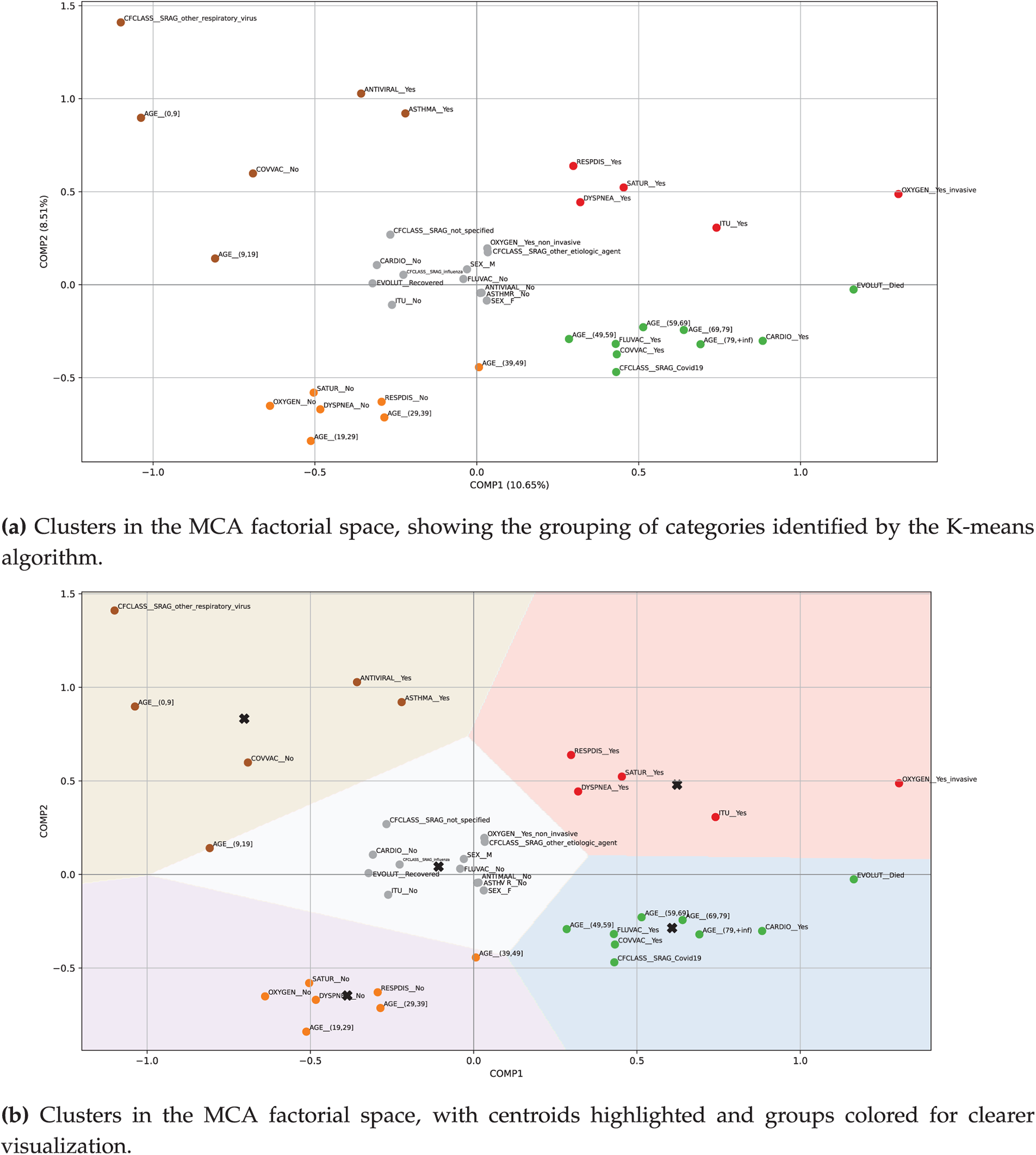
Figure 9: Plots showing the MCA and K-means analysis with five clusters applied to the sample data, where the highlighted categories are distributed as follows according to the corresponding colors— Cluster #1 (upper-left); Cluster #2 (upper-right); Cluster #3 (central); Cluster #4 (lower-left); and Cluster #5 (lower-right). See Table 9 for interpretation

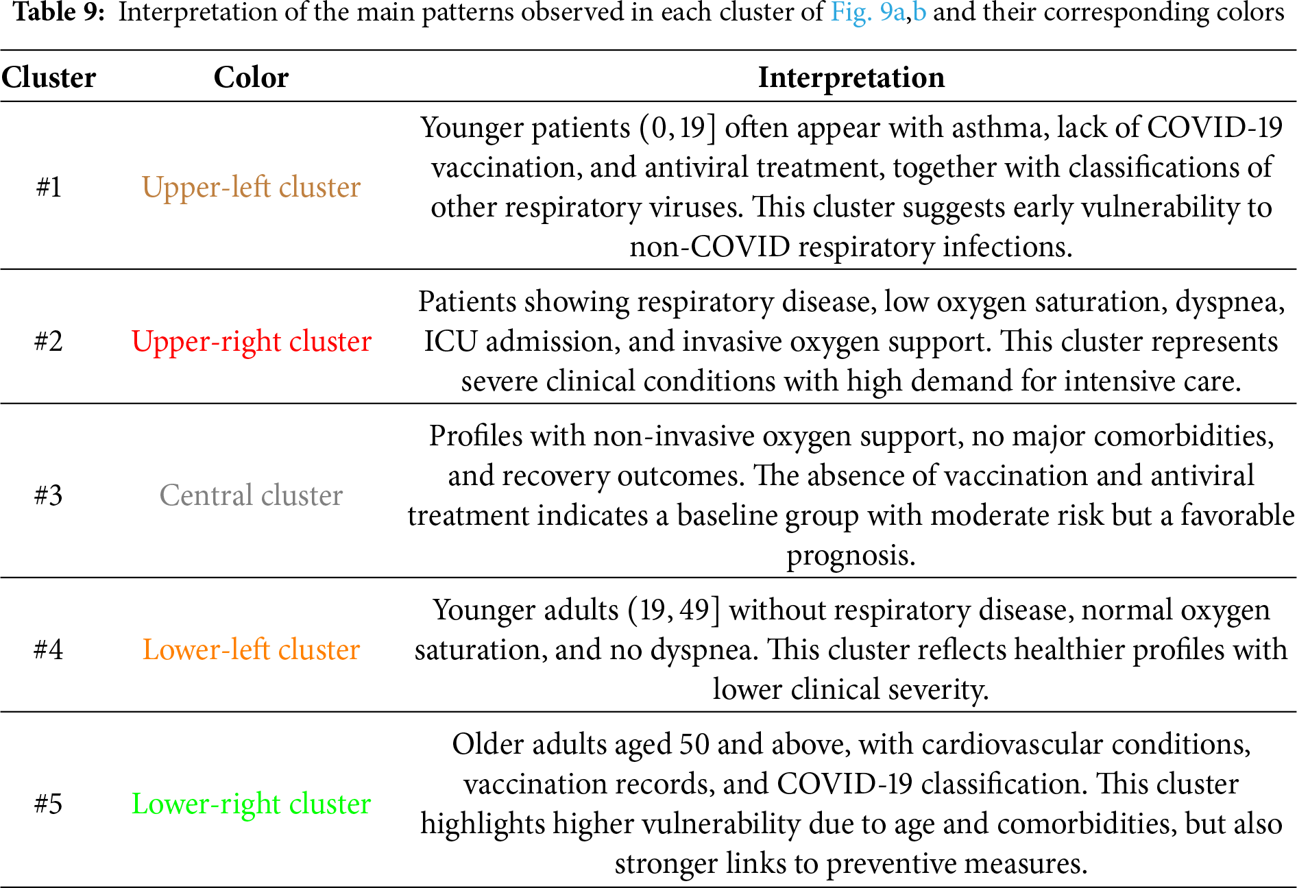
Table 9 summarizes the main patterns identified through MCA and K-means analysis, providing an interpretive description of the most relevant categories grouped within each cluster.

5.3 MCA and K-Means Analysis with Simulated Patients

To address “what-if” questions in our extended proto-DT model using MCA and K-means, we have prepared two types of simulated scenarios. On the one hand, we incorporate new patients generated from the real patient data. On the other hand, we modify the real data by altering the values of some categorical variables.

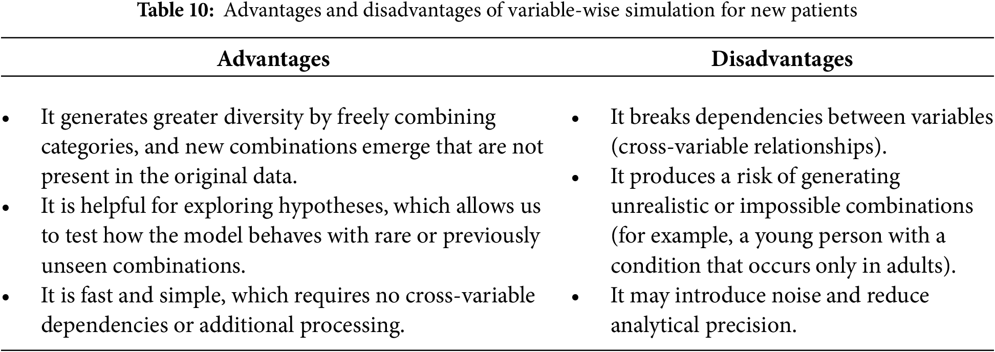
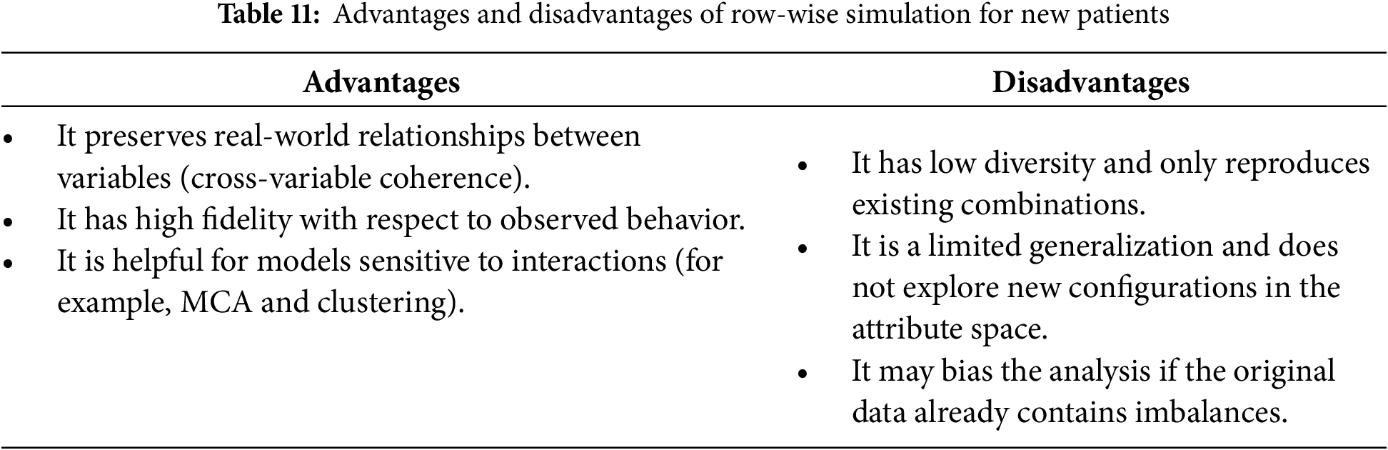
To simulate new patients, we implement two distinct strategies: (i) randomly selecting the values of each variable, a process we refer to as variable-wise simulation, and (ii) selecting variable values collectively based on an existing patient’s profile, which we refer to as row-wise simulation. In both simulations, the value of the EVOLUT variable is predicted using an LR model. Table 10 outlines the strengths and limitations of variable-wise simulation, whereas Table 11 highlights those associated with row-wise simulation.

The two simulation strategies serve complementary purposes. Variable-wise simulation increases diversity by generating novel combinations of attributes, which is helpful for testing the model under rare or atypical scenarios. Row-wise simulation, in contrast, preserves the coherence of real-world variable relationships, ensuring fidelity to observed patient profiles. By applying both strategies, we were able to evaluate the stability of the MCA + K-means clustering under conditions of greater diversity as well as higher fidelity. The fact that the clusters retained their categorical composition across both simulation types reinforces the robustness of the proto-DT framework, showing that clinically meaningful patterns are preserved even when the data is perturbed.

The simulate_by_variable function was implemented to perform variable-wise simulation, while the simulate_by_row function handles row-wise simulation. To integrate these methods, we developed the simulate_patients function.

By combining both strategies, we can leverage the complementary strengths of each simulation: (i) achieving a balance between diversity and realism, (ii) controlling the level of risk associated with the desired data variability, and (iii) enhancing the adequacy of the model by exposing MCA and K-means to a wider range of input data. Fig. 10a shows the categories in the reduced-dimensional space produced by the MCA, incorporating 15% newly simulated patients. The MCA model captured 18.53% of the explained variability. To compare with the analysis based on the original sample, the K-means algorithm was executed using five clusters. Fig. 10b illustrates the category distribution within the reduced-dimensional space derived from the MCA, which includes 30% newly simulated patients. In this configuration, the MCA accounted for 17.61% of the total explained variance, and five clusters were also used.

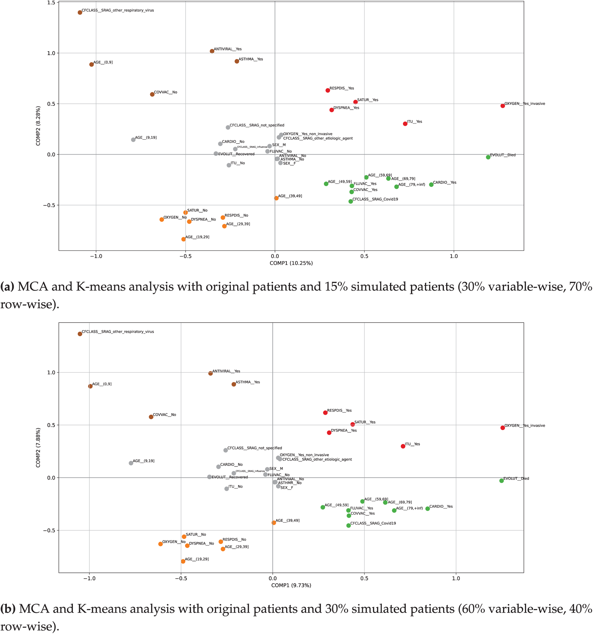
Figure 10: Plots of MCA and K-means analysis incorporating 15% and 30% simulated data, where the highlighted categories are distributed as follows according to the corresponding colors— Cluster #1 (upper-left); Cluster #2 (upper-right); Cluster #3 (central); Cluster #4 (lower-left); and Cluster #5 (lower-right)

When comparing the results generated from the original sample with those obtained through simulations using the proto-DT, the MCA + K-means model appears to be stable, as the new results show only slight variations—indicating that the model is not heavily dependent on the original dataset. Note that the newly simulated patients include realistic cases based on the existing distribution and new clinical scenarios (such as atypical cases, infrequent combinations, or novel patient profiles). This enables the model to learn from a wider range of cases without the need for additional real data. Such capability is essential for training a proto-DT model that can anticipate unusual or rare situations.

Simulations were also conducted by altering the categorical structure of certain variables, following the specifications outlined in Table 6. For this purpose, we developed the Python function simulate_interventions, which simulates the effect of modifying selected clinical variables—such as AGE, ICU, OXYGEN, and COVVAC—in randomly chosen patients, and subsequently updates their clinical outcome (EVOLUT) based on an LR model that estimates the probability of death.

Importantly, the comparison between real and simulated datasets revealed that the categorical composition of the clusters remained unchanged. Only minor positional shifts were observed in the MCA plots, but the overall grouping of patient profiles was preserved. This consistency demonstrates that the proto-DT framework is robust to data perturbations and capable of maintaining clinically coherent clusters even when new synthetic cases are introduced. From a practical perspective, such robustness ensures that the insights derived from the model—such as identifying vulnerable groups or anticipating ICU demand—do not correspond to a particular dataset, but rather reflect stable patterns that can inform clinical and managerial decision-making.

5.4 Further Simulations

We also developed the auxiliary function apply_intervention to support the simulation of interventions. This function randomly selects one to three variables from a set of modifiable clinical attributes—such as AGE, ICU, OXYGEN, and COVVAC—and assigns new values to them, ensuring that each replacement remains within the original variable’s valid category space.

The selected values differ from the original state, thereby introducing realistic patient-level modifications. This randomized yet constrained intervention mechanism permits us to generate alternative patient profiles that reflect possible treatment or condition adjustments. The function apply_intervention operates within the broader simulation framework implemented via simulate_interventions. In the first scenario, we modified 35% of the original patients.

Fig. 11a shows the MCA combined with K-means clustering plot. The first two dimensions captured 17.12% of the total data variability. In a second scenario, we intervened 20% of the patients. The corresponding plot is shown in Fig. 11b. A total of 17.91% of the data variability was captured. As shown in Fig. 11a, the intervention affecting 35% of the original patients did not alter the overall cluster structure but led to specific reassignments of categories. In the upper-left cluster, ASTHMA_yes and COVVAC_no disappeared, narrowing the profile to pediatric respiratory infections with antiviral treatment. In the upper-right cluster, ICU_yes and OXYGEN_Yes_invasive migrated away, while ASTHMA_yes was incorporated, redefining this group as respiratory compromise without ICU or invasive support. The central cluster absorbed COVVAC_no, maintaining its role as a moderate-risk baseline. The lower-left cluster remained unchanged. Therefore, the lower-right cluster gained ICU_yes and OXYGEN_Yes_invasive, consolidating it as the profile of highest clinical severity, combining older age, comorbidities, COVID-19 classification, and fatal outcomes.

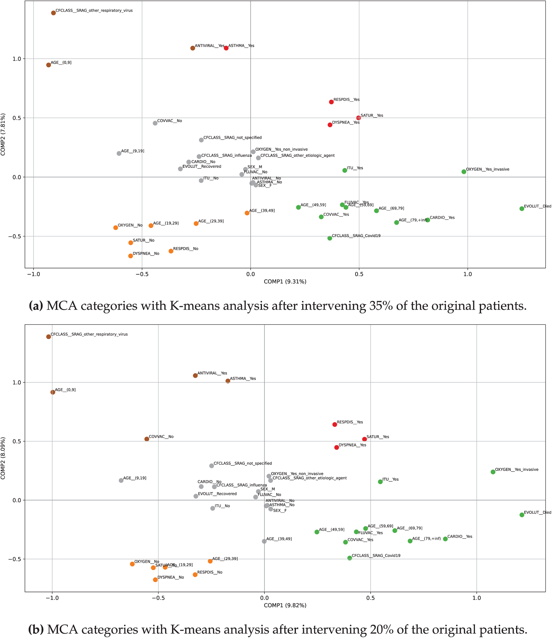
Figure 11: Plots of MCA and K-means clusters after intervening 20% and 35% of the original patients, where the highlighted categories are distributed as follows according to the corresponding colors— Cluster #1 (upper-left); Cluster #2 (upper-right); Cluster #3 (central); Cluster #4 (lower-left); and Cluster #5 (lower-right)

As shown in Fig. 11b, the intervention affecting 20% of the original patients produced only minor adjustments in cluster composition without altering the overall structure. In the upper-left cluster, both ASTHMA_yes and COVVAC_no reappeared, restoring the pediatric profile compared to the 35% intervention. The upper-right cluster was reduced to respiratory compromise variables (RESPDIS_yes, DYSPNEA_yes, SATUR_yes), no longer including asthma. The central cluster expanded its age range by incorporating AGE_(39,49], while the lower-left cluster narrowed to AGE_(19,39] instead of extending to 49 years. The lower-right cluster remained unchanged, consistently concentrating severe cases with older age, comorbidities, COVID-19 classification, fatal outcomes, ICU admission, and invasive oxygen support. These differences suggest that the intervention at 20% redistributed certain categories across clusters but preserved the clinical meaning of each group, reinforcing the robustness of the MCA + K-means method under varying levels of simulated perturbation.

Simulating patient interventions represents a valuable tool for exploring possible scenarios in large-scale categorical datasets. Using the function sim_patients, it is possible to systematically modify a controlled proportion of the sample, preserving the overall structure of the original dataset while introducing variations generated through probabilistic models. This selective intervention capability allows for comparative analysis between observed and modified configurations, as well as sensitivity assessments under varying degrees of change.

When combined with dimensionality reduction techniques such as MCA and clustering methods like K-means, the simulated interventions can be projected onto a reduced space in which emerging groupings, structural shifts, and global effects of the modifications become visually and analytically apparent. Moreover, the modular design of the implemented functions ensures adaptability to diverse modeling strategies, sample sizes, and intervention criteria—making them highly versatile tools for exploratory analysis, hypothesis validation, or scenario simulation in clinical and social research settings. This combination ensures that the analysis is not only technically sound but also meaningful for healthcare professionals and managers, who can use these insights to anticipate patient trajectories and allocate resources more effectively.

The workflow applied here follows a sequential structure. First, MCA and K-means clustering are performed on the real dataset to identify the initial groupings. Next, simulated patients are generated using both variable-wise and row-wise strategies, and the MCA + K-means analysis is repeated to evaluate the stability of the clusters under conditions of increased diversity and fidelity. Therefore, intervention-based simulations are applied by modifying selected categorical variables (such as AGE, ICU, OXYGEN, and COVVAC), followed again by MCA + K-means clustering to assess the robustness of the framework under perturbations. The complete sequence of steps is summarized in Fig. 12, which integrates the analyses on real data, simulated patients, and intervention scenarios, concluding with the generation of plots and interpretive results.

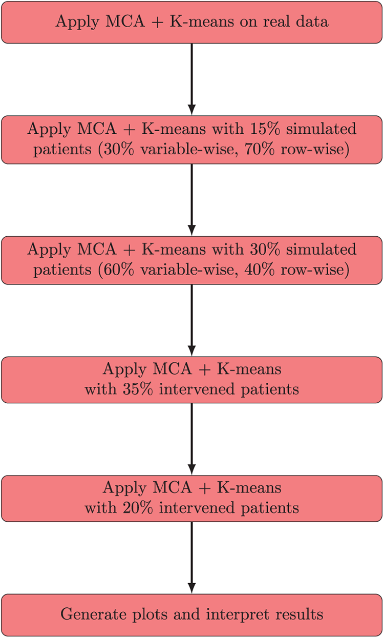
Figure 12: Integrated flowchart summarizing MCA + K-means analysis on real data, simulated patients, and intervention scenarios, concluding with plot generation and interpretation

5.5 Explainability of MCA and K-Means Analysis

The integration of MCA with K-means clustering not only provides a methodological framework for dimensionality reduction and patient grouping but also enhances interpretability. MCA projects categorical variables into a factorial space where associations between attributes become visually accessible, enabling clinicians and researchers to identify coherent patterns.

When combined with K-means, the MCA projections yield clusters that can be directly inspected in terms of patient profiles, categorical combinations, and simulated scenarios. This allows the reader to understand how patient categories are grouped and how simulated data influence the overall clustering structure. Moreover, the simulation strategies introduced—variable-wise and row-wise—strengthen explainability by exposing the model to both novel and realistic patient configurations. Variable-wise simulation allows the exploration of rare or atypical categorical combinations, while row-wise simulation preserves real-world dependencies. The simulation strategies provide interpretable insights into how the MCA + K-means method responds to different patient scenarios, thereby reinforcing the transparency and robustness of the analysis. In this way, our work aligns with recent advances in explainable AI for healthcare, where interpretability is emphasized as a critical component of trustworthy diagnostic systems [46].

In addition, our study highlights two distinct types of simulation, each contributing to explainability in a specific way. Variable-wise and row-wise simulations act by introducing random perturbations or recombinations of categorical variables. Their role is to expose the clustering framework to novel or atypical patient configurations while preserving realistic dependencies. Thus, the clusters remained practically unchanged, showing that the MCA + K-means method is stable and reproducible. From the perspective of explainable AI, this stability demonstrates that the model is trustworthy, allowing researchers to confirm that the variation introduced by simulation does not compromise the interpretability of patient profiles.

Intervention-based simulations act by deliberately modifying a fixed proportion of patients. Although they also rely on random selection, their structured design produced categorical reassignments, with attributes such as ASTHMA_yes, COVVAC_no, ICU_yes, and OXYGEN_Yes_invasive showing changes across simulations. From the perspective of explainable AI, this clinical coherence is crucial as it shows that systematic modifications are transparently reflected in the clustering, enabling analysts to trace how targeted interventions reshape patient grouping in a meaningful and interpretable way. These two types of simulation strategies provide complementary evidence for explainability. Stability under random perturbations ensures reproducibility, while stability with clinically coherent reassignments under structured interventions ensures relevance. This dual contribution aligns with the principles of explainable AI, reinforcing transparency, interpretability, and confidence in the proto-DT framework.

6  Discussion

6.1 Positioning: Proto-DT versus Standard Predictive Models

Unlike typical predictive classifiers that yield only a probability estimate from a single input, the proto-DT framework maintains a patient-specific representation. This framework enables scenario testing and iterative simulation, albeit still using cross-sectional data. As healthcare systems move toward comprehensive electronic health record infrastructures, the proto-DT concept could be augmented with repeated snapshots or streaming data, creating a continuum from static to dynamic DTs. Consequently, our proposed framework addresses a currently underserved domain: using categorical single-point data to provide actionable insights that simulate aspects of a DT.

6.2 Findings and Clinical & Operational Implications

Our findings indicate that even with cross-sectional categorical data, we can build a proto-DT framework that provides risk assessments for respiratory illness. When compared to baseline classification (for example, LR, RF, and XGBoost), DNN achieved a higher recall (0.81), showing its strength in identifying high-risk cases. However, this came at the cost of low precision, implying a high rate of FPs. XGBoost offered higher accuracy overall but missed a greater proportion of mortality cases. LR and RF balanced recall and precision more evenly, illustrating the performance trade-offs in cost-sensitive learning setups. Despite their demonstrated effectiveness, these models rely on a single snapshot of patient data. By definition, they cannot capture disease progression over time or the evolving clinical context. Nonetheless, the scenario-based proto-DT framework reveals how even static categorical features can support “what-if” simulations, providing a novel angle for exploring potential interventions in the absence of longitudinal input. The above-mentioned novel angle extends beyond standard machine learning classification by creating a per-patient virtual profile that can be iteratively updated or queried with hypothetical scenarios. In this sense, our proto-DT framework takes a step forward in building a fully dynamic DT, closing the gap between purely static modeling and continuous real-time updates.

Clinically, the proto-DT framework can support triage decisions, resource allocation, and care planning by simulating how certain interventions—such as early ICU transfer or ensuring vaccination—might influence a patient’s predicted mortality risk. These simulations do not prove causality, but they guide risk assessment and prompt further investigation or monitoring of particular subgroups (such as older unvaccinated patients). The ability to test multiple interventions also helps healthcare administrators to model various resource scenarios (for example, increased ICU beds or modified vaccination coverage) before committing to these interventions in practice.

6.3 Role of Simulations in Explainability

The simulation strategies applied in this study provide complementary insights into the stability and sensitivity of the proto-DT framework. Variable-wise and row-wise simulations introduced random perturbations, demonstrating that the MCA + K-means clustering remained reproducible under atypical patient configurations. In contrast, intervention-based simulations deliberately modified categorical attributes, revealing how targeted changes reshape patient profiles. These methods highlight that our proto-DT framework is not only technically robust but also capable of reflecting clinically relevant shifts, thereby improving transparency and interpretability for healthcare decision-making.

6.4 Broader Impact and Alignment with Sustainable Development Goals

Beyond methodological and clinical contributions, our framework also aligns with broader societal objectives. In particular, it supports SDG 3 (good Health and well-being), by showing how categorical health data can be transformed into actionable risk assessments and scenario-based simulations. This alignment highlights the potential of the proto-DT framework to strengthen preventive care, improve resource allocation, and support care planning in healthcare systems. By enabling more transparent and reproducible analyses, the method also contributes to SDG 9 (industry, innovation, and infrastructure) by advancing innovation in data-driven clinical infrastructures. Emphasizing these alignments expands the relevance of our study to a wider readership and underscores its potential societal impact.

7  Conclusions and Limitations

This study demonstrated that a proto-DT framework—constructed solely from cross-sectional categorical data—can support meaningful scenario-based analyses for patients with severe respiratory infections. By pairing cost-sensitive machine learning with a flexible per-patient representation, we show it is feasible to simulate “what-if” interventions (for example, ICU admission, oxygen support, vaccination status) and gauge their potential impact on mortality risk. Although these scenario tests do not prove causation, they enrich static risk predictions by highlighting how key factors might shift a patient’s risk profile.

Moreover, our proto-DT framework establishes a pathway for transitioning from single snapshots to fully dynamic DTs as additional data becomes available. Future research can improve this framework by incorporating time-series records, external validations, and advanced interpretability methods to provide more specific clinical insights. Despite its current limitations, the proto-DT framework provides a scalable stepping stone toward real-time DT solutions, helping researchers and clinicians to leverage even modest categorical datasets for deeper and more personalized decision support in respiratory healthcare.

The proposed proto-DT framework, enriched through MCA and K-means, showed its potential for revealing latent structures and alternative patient profiles under controlled simulations. This framework facilitates understanding of categorical health data and supports sensitivity-driven modeling in clinical research. In addition, a dedicated Python library was developed to ensure the reproducibility and scalability of the methodology, enabling other researchers to implement, adapt, and expand the proposed framework in their own applications.

Several limitations warrant mention. First, although cost-sensitive learning helped to mitigate class imbalance, the model performance may still be sensitive to data-specific artifacts, biases, or missing confounders. Second, cross-sectional data limit our ability to observe temporal disease trajectories and confirm whether interventions truly alter outcomes. Third, without external validation on other cohorts, the generalizability of our findings to different healthcare contexts or patient populations remains unknown. Nonetheless, our proto-DT framework points to promising future work. Integrating repeated cross-sectional updates or true time-series data could evolve the proto-DT into a near-real-time DT, benefiting from continuous learning as patient states change. Incorporating additional clinical features—such as imaging or lab results—would likely refine risk predictions and reveal “what-if” pathways.

Thus, applying interpretability methods (for example, Shapley additive explanations) to these scenario analyses would enhance transparency, enabling clinicians to see not just predictions but also how each feature drives the model decisions.

Beyond these limitations, this study provides a new understanding of how categorical data can be transformed into proto-DTs that are both interpretable and clinically meaningful. For hospitals and public health systems, this implies that even limited datasets can be converted into actionable insights, supporting patient stratification, early risk identification, and resource allocation in contexts where continuous monitoring is not yet feasible. As a clearer research contribution, we show that categorical proto-DTs can serve as a methodological bridge between static risk models and dynamic DTs.

Note that, while the proto-DT framework demonstrates the utility of categorical surveillance data for population-level scenario analyses, its scope is inherently limited by the absence of vital signs, laboratory values, and severity scores. These constraints define the boundaries of our approach and emphasize its role as a complement to, rather than a replacement for, ICU-based prognostic models.

Acknowledgement: Not applicable.

Funding Statement: The authors received no specific funding for this study.

Author Contributions: Conceptualization: Victor Leiva, Carlos Martin-Barreiro, Viviana Giampaoli; formal analysis: Victor Leiva, Carlos Martin-Barreiro, Viviana Giampaoli; investigation: Victor Leiva, Carlos Martin-Barreiro, Viviana Giampaoli; methodology: Victor Leiva, Carlos Martin-Barreiro, Viviana Giampaoli; validation: Victor Leiva, Carlos Martin-Barreiro, Viviana Giampaoli; writing original draft: Victor Leiva, Carlos Martin-Barreiro, Viviana Giampaoli; writing revision and editing: Victor Leiva, Carlos Martin-Barreiro, Viviana Giampaoli. All authors reviewed the results and approved the final version of the manuscript.

Availability of Data and Materials: The data and code used in this article are available upon request from the authors and are also included within the article.

Ethics Approval: Not applicable.

Conflicts of Interest: The authors declare no conflicts of interest to report regarding the present study.

Appendix A Python Code for Model Training and Scenario-Based Analysis

The listing below contains a representative Python script for reproducing the main steps of our study, that is: (i) data preprocessing, (ii) model training (with cost-sensitive strategies), (iii) evaluation, and (iv) example scenario-based analyses in a proto-DT framework.

The code assumes all required Python libraries (for example, pandas, numpy, scikit-learn, tensorflow, xgboost) are installed, and the dataset is available as described in the main text.

# -------------------

Python code for model training and scenario-based analysis

# -------------------

import logging

import os

from typing import Dict, Iterable

import numpy as np

import pandas as pd

import tensorflow as tf

from sklearn.ensemble import RandomForestClassifier

from sklearn.linear_model import LogisticRegression

from sklearn.metrics import (classification_report, confusion_matrix, roc_auc_score)

from sklearn.model_selection import StratifiedKFold, train_test_split

from sklearn.utils import class_weight

from tensorflow.keras.layers import Dense, Dropout

from tensorflow.keras.models import Sequential

import xgboost as xgb

# -------------------

# 1) Data Loading and Preprocessing

# -------------------

def preprocess_data(df: pd.DataFrame) -> pd.DataFrame:

# -------------------

    Convert relevant columns to categorical, create EVOLUT_BIN (1 if Died, 0 if Recovered),

    create a COVID_status variable, and remove the original EVOLUT and CFCLASS fields.

    Parameters

    ----------

    df : pd.DataFrame

        The raw DataFrame with severe acute respiratory infection records.

    Returns

    -------

    pd.DataFrame

        The preprocessed DataFrame with new columns and dropped unused fields.

# -------------------

    required_cols = [

        "EVOLUT", "CFCLASS", "SEX", "DYSPNEA", "RESPDIS", "SATUR",

        "CARDIO", "ASTHMA", "FLUVAC", "ANTIVIRAL", "ICU", "OXYGEN",

        "AGE", "COVVAC"

    ]

    for col in required_cols:

        if col not in df.columns:

            logging . warning(f"Required column {col} not found in dataset.")

    # Create binary mortality indicator: Died -> 1, else -> 0

    df ["EVOLUT_BIN"] = df ["EVOLUT"].apply(lambda x: 1 if x == "Died" else 0)

    # Create a COVID_status variable

    df ["COVID_status"] = df ["CFCLASS"] . apply(

        lambda x: "COVID" if x == "SRAG_Covid19" else "non-COVID"

    )

    # Convert relevant columns to categorical

    categorical_cols = [

        "SEX", "DYSPNEA", "RESPDIS", "SATUR", "CARDIO", "ASTHMA",

        "FLUVAC", "ANTIVIRAL", "ICU", "OXYGEN", "COVID_status",

        "AGE", "COVVAC"

    ]

    for c in categorical_cols:

        if c in df.columns:

            df [c] = df [c].astype("category")

    df.drop(columns=["EVOLUT", "CFCLASS"], inplace=True, errors="ignore")

    return df

def build_dnn_model(input_dim: int) -> tf.keras.Model:

# -------------------

    Build a simple feed-forward neural network (DNN) in Keras/TensorFlow

    for binary classification.

    Parameters

    ----------

    input_dim : int

        Number of input features (after one-hot encoding).

    Returns

    -------

    tf.keras.Model

        Compiled Keras model ready for training.

# -------------------

    model = Sequential([

        Dense(128, activation="relu", input_shape=(input_dim,)),

        Dropout(0.5),

        Dense(64, activation="relu"),

        Dropout(0.5),

        Dense(1, activation="sigmoid")  # Binary classification output

    ])

    model.compile(optimizer="adam", loss="binary_crossentropy", metrics=["accuracy"])

    return model

# -------------------

# 2) Main Script

# -------------------

def main():

    # (A) Load data

    df = pd.read_excel ("dataAsmaNEWultimate.xlsx")

    logging . info(f"Initial data shape: {df.shape}")

    # (B) Preprocess

    df = preprocess_data(df)

    logging . info(f"Columns after preprocessing: {df.columns.tolist()}")

    logging . info(f"Data shape after preprocessing: {df.shape}")

    # (C) One-Hot Encoding

    categorical_vars = [

        "AGE", "SEX", "DYSPNEA", "RESPDIS", "SATUR", "CARDIO",

        "ASTHMA", "FLUVAC", "ANTIVIRAL", "ICU", "OXYGEN",

        "COVVAC", "COVID_status"

    ]

    X_encoded = pd.get_dummies(df [categorical_vars], drop_first=False)

    y = df ["EVOLUT_BIN"].values.astype(int)

    logging . info(f"Encoded feature matrix shape: {X_encoded.shape}")

    # (D) Train-Test Split

    X_train, X_test, y_train, y_test = train_test_split(

        X_encoded, y, test_size=0.2, random_state=123, stratify=y

    )

    logging . info(f"Training set size: {X_train.shape}, Test set size: {X_test.shape}")

    # (E) Class Weights

    class_labels = np.unique(y_train)

    cw_values = class_weight.compute_class_weight(

        class_weight='balanced', classes=class_labels, y=y_train

    )

    class_weights_dict = {cls: w for cls, w in zip(class_labels, cw_values)}

    logging . info(f"Class weights: {class_weights_dict}")

    # (F) Build and Train DNN Model

    dnn_model = build_dnn_model(X_train.shape [1])

    logging . info(dnn_model.summary())

    # Cross-validation demo

    n_folds = 5

    skf = StratifiedKFold(n_splits=n_folds, shuffle=True, random_state=123)

    for fold, (train_idx, val_idx) in enumerate(skf.split(X_train, y_train), 1):

        logging . info(f"=== Fold {fold}/{n_folds} ===")

        X_train_fold, X_val_fold = X_train.iloc[train_idx], X_train.iloc[val_idx]

        y_train_fold, y_val_fold = y_train[train_idx], y_train[val_idx]

        model_fold = build_dnn_model(X_train.shape [1])

        model_fold.fit(

            X_train_fold, y_train_fold,

            validation_data=(X_val_fold, y_val_fold),

            epochs=5, batch_size=256,

            class_weight=class_weights_dict, verbose=1

        )

    # Training

    dnn_model.fit(

        X_train, y_train,

        validation_split=0.2,

        epochs=100, batch_size=256,

        class_weight=class_weights_dict, verbose=1

    )

    # (G) Evaluation on Test Set

    y_pred_prob = dnn_model.predict(X_test).ravel()

    y_pred_class = (y_pred_prob >= 0.5).astype(int)

    logging . info("\n=== DNN Confusion Matrix ===")

    logging . info(confusion_matrix(y_test, y_pred_class))

    logging . info("\n=== DNN Classification Report ===")

    logging . info(classification_report(y_test, y_pred_class, digits=4))

    logging . info(f"DNN Test AUC: {roc_auc_score(y_test, y_pred_prob):.4f}")

    # -------------------

    # 3) Logistic Regression, Random Forest, XGBoost examples

    # -------------------

    # Logistic Regression

    logging . info("\n=== Logistic Regression ===")

    logit_model = LogisticRegression(

        penalty='l2', class_weight='balanced', max_iter=1000, solver='lbfgs'

    )

    logit_model.fit(X_train, y_train)

    y_logit_prob = logit_model.predict_proba(X_test)[:, 1]

    y_logit_pred = logit_model.predict(X_test)

    logging . info(f"AUC (Logistic Regression): {roc_auc_score(y_test, y_logit_prob):.4f}")

    # Random Forest

    logging . info("\n=== Random Forest ===")

    rf_model = RandomForestClassifier(

        n_estimators=100, class_weight='balanced_subsample', random_state=123

    )

    rf_model.fit(X_train, y_train)

    y_rf_prob = rf_model.predict_proba(X_test)[:, 1]

    logging . info(f"AUC (Random Forest): {roc_auc_score(y_test, y_rf_prob):.4f}")

    # XGBoost

    logging . info("\n=== XGBoost ===")

    def sanitize_feature_names(columns):

        new_cols = []

        for col in columns:

            col_sanitized = (col.replace("(", "").replace(")", "")

                            .replace("[", "").replace("]", "")

                            .replace(",", "_").replace("+", "plus")

                            .replace("<", "lt").replace(">", "gt")

                            .replace(" ", "_"))

            new_cols.append(col_sanitized)

        return new_cols

    X_train_sanit = X_train.copy()

    X_test_sanit = X_test.copy()

    X_train_sanit.columns = sanitize_feature_names(X_train_sanit. columns)

    X_test_sanit.columns = sanitize_feature_names(X_test_sanit. columns)

    xgb_model = xgb.XGBClassifier(

        n_estimators=100, max_depth=6, learning_rate=0.1,

        random_state=123, use_label_encoder=False, eval_metric="logloss"

    )

    xgb_model.fit(X_train_sanit, y_train)

    y_xgb_prob = xgb_model.predict_proba(X_test_sanit)[:, 1]

    logging . info(f"AUC (XGBoost): {roc_auc_score (y_test, y_xgb_prob):.4f}")

    # -------------------

    # 4) Scenario-Based Analyses (Proto-DTs)

    # -------------------

    def proto_digital_twin_scenario(model, base_patient, scenario_changes, all_columns):

# -------------------

        Applies hypothetical interventions to a single patient's feature vector

        and compares the predicted mortality probability before and after the changes.

# -------------------

        base_patient_df = pd.DataFrame([base_patient.values], columns=all_columns).astype("float32")

        base_prob = model.predict(base_patient_df) [0,0]

        scenario_df = base_patient_df.copy(deep=True)

        for col, val in scenario_changes.items():

            scenario_df [col] = np.float32(val)

        scenario_prob = model.predict(scenario_df) [0,0]

        return {

            "base_probability": float(base_prob),

            "scenario_probability": float(scenario_prob)

        }

    def exemplo_proto_gemeo(model, X_test, example_index=100):

# -------------------

        It demonstrates scenario-based changes for a selected patient record.

# -------------------

        base_patient = X_test.iloc[example_index, :]

        all_cols = X_test.columns.tolist()

        logging . info(f"=== Proto-Digital Twin for Patient Index {example_index} ===")

        logging . info(f"Baseline features:\n{base_patient[base_ patient != 0]}")

        # Scenario 1: Vaccinating patient

        scenario_vac = {"COVVAC_No": 0, "COVVAC_Yes": 1}

        res_vac = proto_digital_twin_scenario(model, base_patient, scenario_vac, all_cols)

        logging . info(f"Prob death before = {res_vac['base_ probability']:.4f}")

        logging . info(f"Prob death after  = {res_vac['scenario_ probability']:.4f}")

        # Scenario 2: ICU Admission

        scenario_icu = {"ICU_No": 0, "ICU_Yes": 1}

        res_icu = proto_digital_twin_scenario(model, base_patient, scenario_icu, all_cols)

        logging . info(f"Prob death before = {res_icu['base _probability']:.4f}")

        logging . info(f"Prob death after  = {res_icu['scenario _probability']:.4f}")

    # Run scenario example

    exemplo_proto_gemeo(dnn_model, X_test, example_index=100)

    logging . info("Script completed.")

if __name__ == "__main__":

    logging . basicConfig(level=logging . INFO, format="%(levelname)s: %(message)s")

    main()

Remark.

We use the following commands:

•   build_dnn_model —It creates a simple feed-forward network with two hidden layers and dropout, aiming to mitigate overfitting on a high-dimensional categorical dataset.

•   StratifiedKFold (from scikit-learn) —It demonstrates a five-fold cross-validation procedure. In practice, you may adjust the number of epochs or other hyperparameters to balance runtime and performance.

•   proto_digital_twin_scenario—It illustrates how hypothetical interventions (for instance, setting ICU_Yes = 1) might affect the predicted probability of death, without requiring longitudinal data.

•   Snippet—The snippet also includes examples of training other classifiers (LR, RF, and XGBoost) for a broader comparison.

This code exemplifies the main processes described in the article, that is: (i) data preprocessing, (ii) class imbalance handling, (iii) cross-validation, (iv) model training, (v) evaluation, and (vi) scenario-based (what-if) analyses within a proto-DT framework. By adapting file paths and parameter values, researchers or practitioners can reproduce and extend our methods for other datasets or clinical settings.

Appendix B A Python Library for Proto-DT with MCA and K-Means

# -*- coding: utf-8 -*-

Module for:

- Reading categorical data matrices.

- Fitting and plotting an MCA.

- Evaluating and visualizing K-means clustering on MCA coordinates.

- Training a logistic model with categorical variables (one-hot encoding).

- Simulating new patients (by variable and by row) and applying interventions.

from --future-- import annotations

import random

from pathlib import Path

from typing import Iterable, List, Tuple

import matplotlib.pyplot as plt

import numpy as np

import pandas as pd

import prince

from sklearn.cluster import KMeans

from sklearn.compose import ColumnTransformer

from sklearn.linear_model import LogisticRegression

from sklearn.metrics import silhouette_score

from sklearn.pipeline import Pipeline

from sklearn.preprocessing import OneHotEncoder

# ----------------------------------------------------------------

# Constants

# ----------------------------------------------------------------

RANDOM_STATE: int = 42

DEFAULT_N_COMPONENTS: int = 2

PREDICTOR_VARS: List[str] = [

    "AGE", "SEX", "DYSPNEA", "RESPDIS", "SATUR", "CARDIO",

    "ASTHMA", "FLUVAC", "ANTIVIRAL", "ICU", "OXYGEN",

    "COVVAC", "CFCLASS",

]

TARGET_VAR: str = "EVOLUT"

# ----------------------------------------------------------------

# Data reading utilities

# ----------------------------------------------------------------

def get_datamatrix(path_file: str | Path) -> Tuple[List[str], pd.DataFrame]:

# -------------------

    Reads data from a CSV file separated by ';' and converts all columns to 'category'.

# -------------------

    datamatrix = pd.read_csv(path_file, sep=";")

    columns_names = datamatrix.columns.to_list()

    for col in datamatrix.columns:

        datamatrix[col] = datamatrix[col].astype("category")

    return columns_names, datamatrix

# ----------------------------------------------------------------

# MCA

# ----------------------------------------------------------------

def fit_mca(

    datamatrix: pd.DataFrame,

    n_components: int = DEFAULT_N_COMPONENTS,

    random_state: int = RANDOM_STATE,

) -> prince.MCA:

# ----------------------------------------------------------------

    Fits an MCA model to categorical data.

# ----------------------------------------------------------------

    mca = prince.MCA(n_components=n_components, random_state=random_ state)

    return mca.fit(datamatrix)

def plot_mca_categories(mca: prince.MCA, datamatrix: pd.DataFrame) -> None:

# ----------------------------------------------------------------

    Plots the category coordinates (columns) in the plane of the first two MCA components.

# -------------------

    coords = mca.column_coordinates(datamatrix)

    plt.figure(figsize=(10, 8))

    plt.scatter(coords.iloc[:, 0], coords.iloc[:, 1], color="red")

    offset_x = 0.01

    offset_y = 0.01

    for i, txt in enumerate(coords.index):

        x = coords.iloc[i, 0] + offset_x

        y = coords.iloc[i, 1] + offset_y

        plt.annotate(txt, (x, y), fontsize=7)

    plt.axhline(0, color="grey", lw=1)

    plt.axvline(0, color="grey", lw=1)

    var1 = mca.percentage_of_variance_ [0]

    var2 = mca.percentage_of_variance_ [1]

    plt.xlabel(f"COMP1 ({var1:.2f}%)")

    plt.ylabel(f"COMP2 ({var2:.2f}%)")

    plt.grid(True)

    plt.tight_layout()

    plt.show()

# ----------------------------------------------------------------

# K-means and Elbow/Silhouette curves

# ----------------------------------------------------------------

def elbow_method(coords: pd.DataFrame | np.ndarray, max_k: int = 10) -> None:

# -------------------

    It generates an elbow plot using inertia and silhouette scores for KMeans.

# -------------------

    inertias: List[float] = []

    silhouettes: List[float] = []

    ks = list(range(2, max_k + 1))

    for k in ks:

        kmeans = KMeans(n_clusters=k, random_state=RANDOM_STATE, n_init="auto")

        labels = kmeans.fit_predict(coords)

        inertias.append(kmeans.inertia_)

        silhouettes.append(silhouette_score(coords, labels))

    fig, ax1 = plt.subplots(figsize=(10, 6))

    color1 = "tab:blue"

    ax1.set_xlabel("Number of clusters (k)")

    ax1.set_ylabel("Inertia", color=color1)

    ax1.plot(ks, inertias, marker="o", color=color1, label="Inertia")

    ax1.tick_params(axis="y", labelcolor=color1)

    ax2 = ax1.twinx()

    color2 = "tab:red"

    ax2.set_ylabel("Silhouette Score", color=color2)

    ax2.plot(ks, silhouettes, marker="s", color=color2, label="Silhouette")

    ax2.tick_params(axis="y", labelcolor=color2)

    fig.tight_layout()

    plt.grid(True)

    plt.show()

def plot_kmeans(

    mca: prince.MCA, datamatrix: pd.DataFrame, n_clusters: int

) -> None:

# -------------------

    It generate a cluster plot and centroids using MCA coordinates.

# -------------------

    coords = mca.column_coordinates(datamatrix)

    kmeans = KMeans(n_clusters=n_clusters, random_state=RANDOM_STATE, n_init="auto")

    labels = kmeans.fit_predict(coords)

    centroids = kmeans.cluster_centers_

    x = coords.iloc[:, 0].values

    y = coords.iloc[:, 1].values

    h = 0.005

    x_min, x_max = x.min() - 0.1, x.max() + 0.1

    y_min, y_max = y.min() - 0.1, y.max() + 0.1

    xx, yy = np.meshgrid(

        np.arange(x_min, x_max, h),

        np.arange(y_min, y_max, h),

    )

    Z = kmeans.predict(np.c_[xx.ravel(), yy.ravel()]).reshape (xx.shape)

    plt.figure(figsize=(10, 8))

    plt.contourf(xx, yy, Z, cmap="Pastel1", alpha=0.4)

    plt.scatter(x, y, c=labels, cmap="Set1", s=60)

    offset_x = 0.01

    offset_y = 0.01

    for i, txt in enumerate(coords.index):

        x_txt = coords.iloc[i, 0] + offset_x

        y_txt = coords.iloc[i, 1] + offset_y

        plt.annotate(txt, (x_txt, y_txt), fontsize=7)

    plt.scatter(centroids[:, 0], centroids[:, 1], c="black", s=100, marker="X")

    plt.axhline(0, color="grey", lw=1)

    plt.axvline(0, color="grey", lw=1)

    plt.xlabel("COMP1")

    plt.ylabel("COMP2")

    plt.grid(True)

    plt.tight_layout()

    plt.show()

def cluster_mca_categories(

    mca: prince.MCA, datamatrix: pd.DataFrame, n_clusters: int

) -> None:

# -------------------

    It generates a cluster diagram using the category coordinates obtained from MCA.

# -------------------

    coords = mca.column_coordinates(datamatrix)

    kmeans = KMeans(n_clusters=n_clusters, random_state=RANDOM_STATE, n_init="auto")

    labels = kmeans.fit_predict(coords)

    plt.figure(figsize=(10, 8))

    plt.scatter(coords.iloc[:, 0], coords.iloc[:, 1], c=labels, cmap="Set1", s=60)

    offset_x = 0.01

    offset_y = 0.01

    for i, txt in enumerate(coords.index):

        x = coords.iloc[i, 0] + offset_x

        y = coords.iloc[i, 1] + offset_y

        plt.annotate(txt, (x, y), fontsize=7)

    var1 = mca.percentage_of_variance_ [0]

    var2 = mca.percentage_of_variance_ [1]

    plt.axhline(0, color="grey", lw=1)

    plt.axvline(0, color="grey", lw=1)

    plt.xlabel(f"COMP1 ({var1:.2f}%)")

    plt.ylabel(f"COMP2 ({var2:.2f}%)")

    plt.grid(True)

    plt.tight_layout()

    plt.show()

def evaluate_kmeans_on_categories(

    coords: pd.DataFrame | np.ndarray,

    max_k: int = 10,

    random_state: int = RANDOM_STATE,

) -> pd.DataFrame:

# -------------------

    It evaluates K-means for multiple k values using inertia and silhouette metrics.

# -------------------

    results = []

    for k in range(2, max_k + 1):

        kmeans = KMeans(n_clusters=k, random_state=random_state, n_init="auto")

        labels = kmeans.fit_predict(coords)

        inertia = kmeans.inertia_

        silhouette = silhouette_score(coords, labels)

        results.append({"k": k, "Inertia": inertia, "Silhouette Score": silhouette})

    return pd.DataFrame(results)

# ----------------------------------------------------------------

# Logistic model

# ----------------------------------------------------------------

def logistic_model(datamatrix: pd.DataFrame) -> Pipeline:

# -------------------

    It trains a logistic regression model with one-hot encoding (drop='first')

    using the predictors in PREDICTOR_VARS and EVOLUT as target.

# -------------------

    X = datamatrix[PREDICTOR_VARS]

    y = datamatrix[TARGET_VAR]

    y_bin = (y == "Died").astype(int)

    preprocessor = ColumnTransformer(

        transformers=[

            ("cat", OneHotEncoder(drop="first", handle_unknown="ignore"), PREDICTOR_VARS)

        ])

    model = Pipeline(

        steps=[

            ("preprocessor", preprocessor),

            ("classifier", LogisticRegression(solver="liblinear")),

        ] )

    model.fit(X, y_bin)

    return model

# ----------------------------------------------------------------

# Simulations

# ----------------------------------------------------------------

def simulate_by_variable(

    datamatrix: pd.DataFrame, n: int, model: Pipeline

) -> pd.DataFrame:

# -------------------

    It simulates new patient profiles by randomly sampling categorical values per variable.

    Then predicts EVOLUT with the logistic model.

# -------------------

    simulated = pd.DataFrame()

    for col in datamatrix.columns:

        if col == TARGET_VAR:

            continue

        original_col = datamatrix[col]

        if original_col.dtype.name != "category":

            original_col = original_col.astype("category")

        categories = original_col.cat.categories

        simulated_values = np.random.choice(original_col.dropna(), size=n, replace=True)

        simulated[col] = pd.Categorical(simulated_values, categories=categories)

    y_pred = model.predict(simulated[PREDICTOR_VARS])

    ev_categories = datamatrix[TARGET_VAR].cat.categories

    simulated[TARGET_VAR] = pd.Categorical(

        np.where(y_pred == 1, "Died", "Recovered"), categories=ev_categories

    )

    return simulated

def simulate_by_row(datamatrix: pd.DataFrame, n: int, model: Pipeline) -> pd.DataFrame:

# -------------------

    It simulates new patient profiles by resampling complete rows with replacement.

    Then predicts EVOLUT with the logistic model.

# -------------------

    simulated = (

        datamatrix.drop(columns=[TARGET_VAR]).sample(n, replace=True).reset_index(drop=True)

    )

    for col in simulated.columns:

        if datamatrix[col].dtype.name != "category":

            categories = datamatrix[col].astype("category").cat. categories

        else:

            categories = datamatrix[col].cat.categories

        simulated[col] = pd.Categorical(simulated[col], categories=categories)

    y_pred = model.predict(simulated[PREDICTOR_VARS])

    ev_categories = datamatrix[TARGET_VAR].cat.categories

    simulated[TARGET_VAR] = pd.Categorical(

        np.where(y_pred == 1, "Died", "Recovered"), categories=ev_categories

    )

    return simulated

def simulate_patients(

    datamatrix: pd.DataFrame, total: int, by_variable_ratio: float, model: Pipeline

) -> pd.DataFrame:

# -------------------

    It generates a synthetic patient dataset by combining variable-level and row-level simulations.

# -------------------

    by_variable_n = int(total * by_variable_ratio)

    by_row_n = total - by_variable_n

    sim_var = simulate_by_variable(datamatrix, by_variable_n, model)

    sim_row = simulate_by_row(datamatrix, by_row_n, model)

    simulatedmatrix = pd.concat([sim_var, sim_row], ignore_index=True)

    return simulatedmatrix

def apply_intervention(

    patient: pd.Series,

    intervention_vars: Iterable[str],

    category_map: dict[str, List],

) -> pd.Series | None:

# -------------------

    It simulates an intervention by randomly changing 1 to 3 selected categorical variables.

# -------------------

    modified = patient.copy()

    changes_done = 0

    vars_to_change = random.sample(

        list(intervention_vars), random.randint(1, min(3, len(list(intervention_vars))))

    )

    for var in vars_to_change:

        current_value = patient[var]

        possible_values = category_map[var]

        alternatives = [val for val in possible_values if val != current_value]

        if alternatives:

            new_value = random.choice(alternatives)

            modified[var] = new_value

            changes_done += 1

    return modified if changes_done > 0 else None

def simulate_interventions(

    datamatrix: pd.DataFrame,

    model: Pipeline,

    n_patients: int = 100,

    random_state: int = RANDOM_STATE,

) -> pd.DataFrame:

# -------------------

    It applies simulated interventions to a sample of patients and updates their EVOLUT

    prediction using the logistic model.

# -------------------

    np.random.seed(random_state)

    random.seed(random_state)

    intervention_vars = ["AGE", "ICU", "OXYGEN", "COVVAC"]

    category_map = {

        var: datamatrix[var].astype("category").cat.categories.tolist()

        for var in intervention_vars

    }

    selected_indices = np.random.choice(datamatrix.index, size=n_patients, replace=False)

    for idx in selected_indices:

        original = datamatrix.loc[idx]

        modified = apply_intervention(original, intervention_vars, category_map)

        if modified is not None:

            for var in intervention_vars:

                datamatrix.at[idx, var] = modified[var]

            X_new = pd.DataFrame([datamatrix.loc[idx, PREDICTOR_VARS]])

            proba = model.predict_proba(X_new) [0,1]

            datamatrix.at[idx, TARGET_VAR] = "Died" if proba >= 0.5 else "Recovered"

    return datamatrix

def plot_mca_original_vs_simulated(

    mca_model: prince.MCA,

    original_data: pd.DataFrame,

    simulated_data: pd.DataFrame,

) -> None:

# -------------------

    It visualizes MCA projections of original vs. simulated patients to assess structural similarity.

# -------------------

    original_coords = mca_model.transform(original_data)

    simulated_coords = mca_model.transform(simulated_data)

    plt.figure(figsize=(10, 8))

    plt.scatter(

        original_coords.iloc[:, 0],

        original_coords.iloc[:, 1],

        c="blue",

        label="Original",

        alpha=0.6,

    )

    plt.scatter(

        simulated_coords.iloc[:, 0],

        simulated_coords.iloc[:, 1],

        c="orange",

        label="Simulated",

        alpha=0.6,

    )

    plt.axhline(0, color="grey", lw=1)

    plt.axvline(0, color="grey", lw=1)

    var1 = mca_model.percentage_of_variance_ [0]

    var2 = mca_model.percentage_of_variance_ [1]

    plt.xlabel(f"COMP1 ({var1:.2f}%)")

    plt.ylabel(f"COMP2 ({var2:.2f}%)")

    plt.legend()

    plt.grid(True)

    plt.tight_layout()

    plt.show()

def sim_new_patients(

    datamatrix: pd.DataFrame,

    per_n: float,

    per_var: float,

    model: Pipeline,

    mca_original: prince.MCA,

    n_clusters: int,

) -> None:

# -------------------

    It simulates new patients and plots:

      1) MCA projection of original vs. simulated.

      2) Clusters on the combined matrix.

# -------------------

    total_to_simulate = int(len(datamatrix) * per_n)

    simulatedmatrix = simulate_patients(datamatrix, total_to_simulate, per_var, model)

    combined_matrix = pd.concat([datamatrix, simulatedmatrix], ignore_index=True)

    plot_mca_original_vs_simulated(mca_original, datamatrix, simulatedmatrix)

    mca_simulated = fit_mca(combined_matrix)

    cluster_mca_categories(mca_simulated, combined_matrix, n_clusters)

def sim_patients(

    datamatrix: pd.DataFrame,

    per_n: float,

    model: Pipeline,

    n_clusters: int,

) -> None:

# -------------------

    It modifies (intervenes) a subset of original patients and plots the resulting clusters.

# -------------------

    n_to_modify = int(len(datamatrix) * per_n)

    datamatrix_modified = simulate_interventions(

        datamatrix, model, n_patients=n_to_modify, random_state=RANDOM_STATE

    )

    mca_simulated = fit_mca(datamatrix_modified)

    cluster_mca_categories(mca_simulated, datamatrix_modified, n_clusters)

# ----------------------------------------------------------------

# Main script (example usage)

# ----------------------------------------------------------------

if __name__ == "__main__":

    # Example of how to use the module (adjust file paths and parameters)

    path = "path/to/your_dataset.csv"

    _, df = get_datamatrix(path)

    mca_model = fit_mca(df)

    plot_mca_categories(mca_model, df)

    coords = mca_model.column_coordinates(df)

    elbow_method(coords, max_k=10)

    plot_kmeans(mca_model, df, n_clusters=3)

    model = logistic_model(df)

    sim_new_patients(df, per_n=0.5, per_var=0.6, model=model, mca_original=mca_model, n_clusters=3)

    sim_patients(df, per_n=0.3, model=model, n_clusters=3)

The following lines of code must be executed to reproduce the simulations carried out in this work:

columns_names, datamatrix = get_datamatrix(r"dbAsthma.csv")

mca_original = MCA(datamatrix)

plot_mca_categories(mca_original, datamatrix)

coords = mca_original.column_coordinates(datamatrix)

table_elbow = evaluate_kmeans_on_categories(coords)

print(table_elbow)

elbow_method(coords, max_k = 10)

cluster_mca_categories(mca_original, datamatrix, n_clusters = 5)

plot_kmeans(mca_original, datamatrix, 5)

columns_names, datamatrix = get_datamatrix(r"dbAsthma.csv")

lm = logistic_model(datamatrix)

mca_original = MCA(datamatrix)

sim_new_patients(datamatrix, 0.15, 0.30, lm, mca_original, 5)

sim_new_patients(datamatrix, 0.30, 0.60, lm, mca_original, 5)

columns_names, datamatrix = get_datamatrix(r"dbAsthma.csv")

lm = logistic_model(datamatrix)

mca_original = MCA(datamatrix)

sim_patients(datamatrix, 0.35, lm, 5)

sim_patients(datamatrix, 0.20, lm, 5)

References

1. Ambalarajan V, Mallela MA, Sivakumar V, Dhandapani PB, Leiva V, Martin-Barreiro C, et al. A six-compartment model for COVID-19 with transmission dynamics and public health strategies. Sci Rep. 2024;14:22226. doi:10.1038/s41598-024-72487-9. [Google Scholar] [PubMed] [CrossRef]

2. Rahman MZU, Akbar MA, Leiva V, Martin-Barreiro C, Imran M, Riaz MT, et al. An IoT-fuzzy intelligent approach for holistic management of COVID-19 patients. Heliyon. 2024;10(1):e22454. doi:10.1016/j.heliyon.2023.e22454. [Google Scholar] [PubMed] [CrossRef]

3. Martin-Barreiro C, Cabezas X, Leiva V, Ramos de Santis P, Ramirez-Figueroa JA, Delgado E. Statistical characterization of vaccinated cases and deaths due to COVID-19: methodology and case study in South America. AIMS Math. 2023;8:22693–713. doi:10.3934/math.20231155. [Google Scholar] [CrossRef]

4. Chen D, AlNajem NA, Shorfuzzaman M. Digital twins to fight against COVID-19 pandemic. Internet Things Cyber Phys Syst. 2022;2:70–81. doi:10.1016/j.iotcps.2022.05.003. [Google Scholar] [CrossRef]

5. Ahmed I, Ahmad M, Jeon G. Integrating digital twins and deep learning for medical image analysis in the era of COVID-19. Virtual Real Intell Hardw. 2022;4:292–305. doi:10.1016/j.vrih.2022.03.002. [Google Scholar] [CrossRef]

6. Khan A, Milne-Ives M, Meinert E, Iyawa GE, Jones RB, Josephraj AN. A scoping review of digital twins in the context of the COVID-19 pandemic. Biomed Eng Comput Biol. 2022;13:1–11. doi:10.1177/11795972221102115. [Google Scholar] [PubMed] [CrossRef]

7. Rahman MZU, Akbar MA, Leiva V, Tahir A, Riaz MT, Martin-Barreiro C. An intelligent health monitoring and diagnosis system based on the internet of things and fuzzy logic for cardiac arrhythmia COVID-19 patients. Comput Biol Med. 2023;154:106583. doi:10.1016/j.compbiomed.2023.106583. [Google Scholar] [PubMed] [CrossRef]

8. Jamshidi MB, Hoang DT, Nguyen DN, Niyato D. Revolutionizing biological digital twins: integrating internet of bio-nano things, convolutional neural networks, and federated learning. Comput Biol Med. 2025;188:109970. doi:10.1016/j.compbiomed.2025.109970. [Google Scholar] [PubMed] [CrossRef]

9. Ju H, Cui Y, Su Q, Juan L, Manavalan B. CODENET: a deep learning model for COVID-19 detection. Comput Biol Med. 2024;168:107730. doi:10.1016/j.compbiomed.2024.108229. [Google Scholar] [PubMed] [CrossRef]

10. Wang L, Liu H, Zhang F, Guo L, Chen Z. Intelligent prediction approach of spatial structure response and performance deterioration by integrating spatiotemporal deep learning and digital twins. Eng Struct. 2025;324:119367. doi:10.1016/j.engstruct.2024.119367. [Google Scholar] [CrossRef]

11. Daniell J, Kobayashi K, Alajo A, Alam SB. Digital twin-centered hybrid data-driven multi-stage deep learning framework for enhanced nuclear reactor power prediction. Energy AI. 2025;19:100450. doi:10.1016/j.egyai.2024.100450. [Google Scholar] [CrossRef]

12. Ming Z, Tang B, Deng L, Yang Q, Li Q. Digital twin-assisted fault diagnosis framework for rolling bearings under imbalanced data. Appl Soft Comput. 2025;168:112528. doi:10.1016/j.asoc.2024.112528. [Google Scholar] [CrossRef]

13. Liu Z, Chen K, Wang S, Xiao Y, Zhang G. Deep learning in surgical process modeling: a systematic review of workflow recognition. J Biomed Inform. 2025;162:104779. doi:10.1016/j.jbi.2025.104779. [Google Scholar] [PubMed] [CrossRef]

14. Vidyalakshmi G, Kumar S, Pandey R. Digital twins and cyber-physical systems: a new frontier. Comput Model Eng Sci. 2025;143:15–30. doi:10.32604/cmes.2025.057788. [Google Scholar] [CrossRef]

15. Alrashed S, Min-Allah N, Ali I, Mehmood R. COVID-19 outbreak and the role of digital twin. Multimed Tools Appl. 2022;81:26857–71. doi:10.1007/s11042-021-11664-8. [Google Scholar] [PubMed] [CrossRef]

16. HamlAbadi KG, Vahdati M, Saghiri AM, Gholizadeh K. Digital twins for allergies. In: Digital twin for healthcare. New York, NY, USA: Academic Press; 2023. p. 325–46. doi:10.1016/b978-0-32-399163-6.00021-4. [Google Scholar] [CrossRef]

17. Nancy RG, Venkatesan R, Sundar GN, Jebaseeli TJ. A framework of digital twins for improving respiratory health and healthcare measures. Scalable Comput Pract Exp. 2024;25:3214–23. doi:10.12694/scpe.v25i4.2940. [Google Scholar] [CrossRef]

18. Sun T, Chen H, Zhang Y. Digital twin in healthcare: recent updates and challenges. Front Public Health. 2023;11:1193842. doi:10.1177/20552076221149651. [Google Scholar] [PubMed] [CrossRef]

19. Liu R, Li H, Lv Z. Modeling methods of 3D model in digital twins. Comput Model Eng Sci. 2023;137:101–19. doi:10.32604/cmes.2023.023154. [Google Scholar] [CrossRef]

20. Demuth S, Neumann T, Krefting D. Digital representation of patients as medical digital twins: a framework for interoperability and personalized healthcare. JMIR Med Inform. 2025;13:e54321. doi:10.2196/53542. [Google Scholar] [PubMed] [CrossRef]

21. Zhang K, Zhou HY, Baptista-Hon DT, Gao Y, Liu X, Oermann E, et al. Concepts and applications of digital twins in healthcare and medicine. Patterns. 2024;5:101028. doi:10.1016/j.patter.2024.101028. [Google Scholar] [PubMed] [CrossRef]

22. Andrès E, Escobar C, Doi K. Machine learning and artificial intelligence in clinical medicine—trends, impact, and future directions. J Clin Med. 2025;14(22):8137. doi:10.3390/jcm14228137. [Google Scholar] [PubMed] [CrossRef]

23. Nor AKM, Pedapati SR, Muhammad M, Leiva V. Overview of explainable artificial intelligence for prognostic and health management of industrial assets based on preferred reporting items for systematic reviews and meta-analyses. Sensors. 2021;21(23):8020. doi:10.3390/s21238020. [Google Scholar] [PubMed] [CrossRef]

24. Alkhanbouli R, Matar Abdulla Almadhaani H, Alhosani F, Simsekler MCE. The role of explainable artificial intelligence in disease prediction: a systematic literature review and future research directions. BMC Med Inform Decis Mak. 2025;25(1):110. doi:10.1186/s12911-025-02944-6. [Google Scholar] [PubMed] [CrossRef]

25. Frasca M, La Torre D, Pravettoni G, Cutica I. Explainable and interpretable artificial intelligence in medicine: a systematic bibliometric review. Discov Artif Intell. 2024;4:15. doi:10.1007/s44163-024-00114-7. [Google Scholar] [CrossRef]

26. Jameil AK, Al-Raweshidy H. A digital twin framework for real-time healthcare monitoring: leveraging AI and secure systems for enhanced patient outcomes. Discov Internet Things. 2025;5:37. doi:10.1007/s43926-025-00135-3. [Google Scholar] [CrossRef]

27. Ringeval M, Etindele Sosso FA, Cousineau M, Paré G. Advancing health care with digital twins: meta-review of applications and implementation challenges. J Med Internet Res. 2025;27:e69544. doi:10.2196/69544. [Google Scholar] [PubMed] [CrossRef]

28. Fahim YA, Hasani IW, Kabba S, Ragab WM. Artificial intelligence in healthcare and medicine: clinical applications, therapeutic advances, and future perspectives. Eur J Med Res. 2025;30(1):848. doi:10.1186/s40001-025-03196-w. [Google Scholar] [PubMed] [CrossRef]

29. Quilodrán-Casas C, Silva VLS, Arcucci R, Heaney CE, Guo Y. Digital twins based on bidirectional LSTM and GAN for modelling the COVID-19 pandemic. Neurocomputing. 2022;470:11–28. doi:10.1016/j.neucom.2021.10.043. [Google Scholar] [PubMed] [CrossRef]

30. Molnar C. Interpretable machine learning 2020 [Internet]. [cited 2025 Dec 23]. Available from: https://christophm.github.io/interpretable-ml-book/. [Google Scholar]

31. Brazilian Ministry of Health. Severe acute respiratory infections data–2021 and 2022. Publicly accessible dataset, 2022 [Internet]. [cited 2025 Dec 23]. Available from: https://dados.gov.br/dados/conjuntos-dados/srag-2021-e-2022. [Google Scholar]

32. Gao J, Zhong L, Wu M, Ji J, Liu Z, Wang C, et al. Risk factors for mortality in critically ill patients with COVID-19: a multicenter retrospective case-control study. BMC Infect Dis. 2021;21(1):602. doi:10.21203/rs.3.rs-80661/v1. [Google Scholar] [CrossRef]

33. Becerra-Muñoz VM, Núñez-Gil IJ, Eid CM, Garcia Aguado M, Romero R, Huang J, et al. Clinical profile and predictors of in-hospital mortality among older patients hospitalised for COVID-19. Age Ageing. 2021;50:326–34. doi:10.1093/ageing/afaa258. [Google Scholar] [PubMed] [CrossRef]

34. Buttia C, Llanaj E, Raeisi-Dehkordi H, Kastrati L, Amiri M, Mecani R, et al. Prognostic models in COVID-19 infection that predict severity: a systematic review. Eur J Epidemiol. 2023;38(4):355–72. doi:10.1007/s10654-023-00973-x. [Google Scholar] [PubMed] [CrossRef]

35. Patrascu R, Dumitru CS, Laza R, Besliu RS, Gug M, Zara F, et al. The role of age and comorbidity interactions in COVID-19 mortality: insights from cardiac and pulmonary conditions. J Clin Med. 2024;13(24):7510. doi:10.3390/jcm13247510. [Google Scholar] [PubMed] [CrossRef]

36. Kaya MG, Karaman K. Clinical parameters associated with mortality in elderly patients with COVID-19. PLoS One. 2025;20(9):e0332800. doi:10.1371/journal.pone.0332800. [Google Scholar] [PubMed] [CrossRef]

37. Elkan C. The foundations of cost-sensitive learning. In: Proceedings of the 17th International Joint Conference on Artificial Intelligence. East Sussex, UK: Lawrence Erlbaum Associates Ltd.; 2001. p. 973–8. [Google Scholar]

38. Chawla NV, Bowyer KW, Hall LO, Kegelmeyer WP. Smote: synthetic minority over-sampling technique. J Artif Intell Res. 2002;16:321–57. doi:10.1613/jair.953. [Google Scholar] [CrossRef]

39. Chen T, Guestrin C. XGBoost: a scalable tree boosting system. In: Proceedings of the 22nd ACM SIGKDD International Conference on Knowledge Discovery and Data Mining. New York, NY, USA: ACM; 2016. p. 785–94. [Google Scholar]

40. Freedman DA. Statistical models: theory and practice. Cambridge, UK: Cambridge University Press; 2009. [Google Scholar]

41. Breiman L. Random forests. Mach Learn. 2001;45:5–32. doi:10.1023/a:1010933404324. [Google Scholar] [CrossRef]

42. Bergstra J, Bengio Y. Random search for hyper-parameter optimization. J Mach Learn Res. 2012;13:281–305. [Google Scholar]

43. Srivastava N, Hinton G, Krizhevsky A, Sutskever I, Salakhutdinov R. Dropout: a simple way to prevent neural networks from overfitting. J Mach Learn Res. 2014;15:1929–58. [Google Scholar]

44. Goodfellow I, Bengio Y, Courville A. Deep learning. Cambridge, MA, USA: MIT Press; 2016. [Google Scholar]

45. Kingma DP, Ba J. Adam: a method for stochastic optimization. arXiv:1412.6980. 2015. [Google Scholar]

46. Dharmarathne G, Bogahawaththa M, McAfee M, Rathnayake U, Meddage DPP. On the diagnosis of chronic kidney disease using a machine learning-based interface with explainable artificial intelligence. Intell Syst Appl. 2024;22:200397. doi:10.1016/j.iswa.2024.200397. [Google Scholar] [CrossRef]