
 Submit a Paper
 Propose a Special lssue
 Open Access
ARTICLE

Multiphysics Implicit Coupling Method for Fluid, Particles, and Large-Deformation Structures
1 School of Mechanical Engineering and Automation, Northeastern University, Shenyang, China
2 Mining Hydraulic Technology and Equipment Engineering Research Center, Liaoning Technical University, Fuxin, China
* Corresponding Author: Hualong Xie. Email:
(This article belongs to the Special Issue: Fast Modelling of Fluid-Structure Interaction Based on Computations and Experiments)
Computer Modeling in Engineering & Sciences 2026, 146(2), 12 https://doi.org/10.32604/cmes.2026.075270
Received 28 October 2025; Accepted 28 January 2026; Issue published 26 February 2026
 View Full Text
 Download PDF
Abstract
This study presents an implicit multiphysics coupling method integrating Computational Fluid Dynamics (CFD), the Multiphase Particle-in-Cell (MPPIC) model, and the Finite Element Method (FEM), implemented with OpenFOAM, CalculiX, and preCICE to simulate fluid-particle-structure interactions with large deformations. Mesh motion in the fluid field is handled using the radial basis function (RBF) method. The particle phase is modeled by MPPIC, where fluid-particle interaction is described through momentum exchange, and inter-particle collisions are characterized by collision stress. The structural field is solved by nonlinear FEM to capture large deformations induced by geometric nonlinearity. Coupling among fields is realized through a partitioned, parallel, and non-intrusive iterative strategy, ensuring stable transfer and convergence of interface forces and displacements. Notably, the influence of particles on the structure is not direct but mediated by the fluid, while structural motion directly affects particle dynamics. The results demonstrate that the proposed approach effectively captures multiphysics interaction processes and provides a valuable reference for numerical modeling of coupled fluid-particle-structure systems.Keywords
Supplementary Material
Supplementary Material FileIn modern science and engineering, the study of multiphysics coupling problems has become a key approach for addressing complex engineering issues. Especially in multiphysics systems involving fluid, particle motion, and large deformation structures, the physical complexity increases significantly, giving rise to Fluid-Particle-Structure Interaction (FPSI) problems [1]. Such multiphysics coupling problems are often accompanied by strong nonlinear characteristics, including collisions and friction between particles, bidirectional coupling between particles and fluids, large deformation contact/collision between particles and structures, as well as nonlinear responses such as large displacements and large strains of the structures themselves. They are widely present in fields such as geological engineering, aerospace, and biomechanics. Accurately and efficiently simulating such complex systems is crucial for in-depth understanding of their physical mechanisms, optimizing engineering designs, predicting system behavior, and ensuring operational safety.
Multiphysics coupling simulation has gradually become an essential tool for investigating complex systems, especially in the research of fluid-particle-structure coupling, where it has become an indispensable analytical method. However, for the multiphysics modeling of fluid-particle-structure interactions, researchers often simplify it into three forms: Fluid Particle Interaction (FPI) [2,3], Fluid Structure Interaction (FSI) [4,5], and Particle Structure Interaction (PSI) [6]. It has been widely applied in numerical simulations of fluid-particle, fluid-structure, and particle-structure couplings.
Fluid-particle coupling is primarily used to investigate the motion and interaction of particles in fluids, with broad applications in processes such as fluidized bed reactor design [7] and pulverized coal combustion [8]. In fluid-structure coupling, numerical simulations are employed to analyze the forces exerted by fluids on structures and the resulting deformations, which are applied in studies of wing and parachute stability [9–11], the responses of offshore platforms and ships in ocean engineering [12,13], as well as the stability assessment of bridges and dams under flood or wind loads [14]. Particle-structure coupling mainly focuses on the impact and contact forces of particles on structures, and is widely applied in analyzing the effects of landslides and debris flows on buildings [15], investigating wear in particle conveying equipment [16], and examining the impact and wear behavior of particles on mechanical components in mechanical engineering [17]. These coupling simulations provide important theoretical foundations and technical support for understanding and optimizing complex systems.
Some of the aforementioned two-field coupling problems are essentially FPSI problems. However, in the process of establishing physical models, researchers often neglect one of the physical fields, simplifying the FPSI problem into FSI, PSI, or PFI. In FPSI multiphysics coupling problems, the fluid influences the trajectories and distribution of particles through hydrodynamic effects, while the particle motion, in turn, exerts feedback on the fluid flow field. The contact and impact forces between particles and structures induce structural deformation, which subsequently alters the fluid flow path and the distribution of particles. Simplifying FPSI multiphysics coupling problems into two-field coupling problems is insufficient to meet practical demands.
In the numerical simulation of multiphysics coupling problems, the Monolithic Method and the Partitioned Method are the two mainstream coupling strategies [18,19]. The monolithic method models all coupled physical fields uniformly and, after discretization, forms a large coupled equation system, which is solved as a whole. This approach enables synchronous solution of different physical fields within the same time step, eliminating temporal lag and thus offering high numerical stability and accuracy. It is particularly suitable for problems with strong inter-field coupling effects, such as FSI involving severe structural deformation induced by high-speed flows. However, multiphysics systems often exhibit significant differences in time scales and constitutive properties, which may lead to ill-conditioned matrices during the solution process. Especially for large-scale problems, the governing equations of the system typically involve high-order matrices, resulting in substantially increased computational costs [20]. In addition, the monolithic method requires customized construction of unified governing equations, making it difficult to reuse mature single-field dedicated solvers, thereby limiting the rapid integration of the latest advances across disciplines.
In contrast, the partitioned method is a more flexible coupling strategy that divides different physical fields into independent subsystems, each solved with dedicated solvers, while information exchange and coupling are achieved through boundary conditions. The greatest advantage of the partitioned method lies in its strong modularity and reusability, allowing for the full utilization of existing mature numerical solvers. Depending on the frequency of boundary data exchange and the coupling strength, the partitioned method can be further classified into explicit and implicit coupling schemes. Explicit coupling is easy to implement and computationally efficient; however, it may cause numerical instability when dealing with strongly coupled problems or cases with high density ratios. Explicit coupling methods can usually be stably solved in gases, but may be unstable in liquids. This is because when the densities of the structure and the fluid are comparable, the added-mass effect between the fluid and the solid can lead to numerical instabilities [21–23]. By contrast, implicit coupling employs iterative procedures (e.g., Aitken iteration method, Newton/Quasi-Newton iteration method, or Gauss–Seidel iteration method) within each time step to ensure that the coupling variables between different physical fields satisfy convergence criteria, thereby improving the accuracy of coupled analyses. Although this iterative strategy enhances stability, it requires multiple physical inter-field iterations at each time step, leading to higher computational costs [24].
In multiphysics coupling problems, the integration strategies of partitioned coupling solvers are generally classified into intrusive and non-intrusive approaches [25,26]. The intrusive method requires in-depth modifications to the solvers of each sub-physics field, embedding the coupling and iteration methods into the physics field solvers. Such methods involve high development complexity, lack flexibility, and make it difficult to reuse existing software resources. In contrast, non-intrusive solvers adopt a modular approach, typically treating the physical field solver as a black-box solver. The coupling solver is modeled separately and exchanges information (e.g., boundary conditions or source terms) through interfaces, thereby preserving the independence of each field solver. This approach facilitates the integration of existing mature single physics field solvers, requires less development effort, and offers good generality and scalability.
According to the scheduling strategy among different physical fields, multiphysics coupling methods can be classified into parallel coupling and serial coupling [27]. In the serial coupling approach, the physical fields are solved sequentially in a prescribed order, update the physical field state one by one at each time step. This method is relatively simple to implement and easy to control the solution process, making it suitable for weakly coupled systems or systems with similar time scales. However, the efficiency of serial coupling is relatively low, since the total computational time is approximately the sum of the runtimes of all field solvers. In contrast, the parallel coupling approach solves all physical fields simultaneously within each time step, with real-time information exchange through coupling interfaces [28,29]. This method avoids time lag, provides higher accuracy and stronger stability, and is suitable for strongly coupled or highly nonlinear systems. The computational efficiency of parallel coupling is relatively higher, as the total runtime is approximately equal to the maximum runtime consumed by a single physical field solver. It should be noted that the parallel coupling method described here is different from the internal parallelization of fluid, solid, or particle solvers, the two concepts are not the same.
Regarding the FPSI issue, current research mainly focuses on areas such as particle-laden pipe flows and particle flow impacts on structures. Leonardi et al. [30] developed an FPSI coupling method based on Lattice Boltzmann Method (LBM)-Discrete Element Method (DEM)-FEM to investigate the impact resistance of flexible barriers against debris flows. Jonsén et al. [31] established a multiphysics coupling model using Smoothed Particle Hydrodynamics (SPH)-DEM-FEM to study the interactions among slurry, grinding balls, and the ball mill. Similarly, Larsson et al. [32] conducted research on this using a Particle Finite Element Method (PFEM)-DEM-FEM coupling model. Liu et al. [1] adopted an SPH-DEM-FEM method to predict structural damage caused by debris flow impacts on buildings. These FPSI coupling models are all overall, intrusive, and serial coupling approaches, which results in the FPSI coupling models applying only to specific scenarios and reducing their flexibility in broader applications. Yao et al. [33] proposed a CFD-FEM-DEM coupling method to investigate pipeline vibrations induced by sand-laden fracturing fluids. In this method, ANSYS was employed to simulate the coupling between the fluid and the geometrically nonlinear structure, while EDEM was used to resolve particle motion. This approach belongs to the category of partitioned, implicit, non-intrusive, and serial coupling. However, since the structural domain deformation in this model is relatively small, it is not suitable for analyzing FPSI problems involving large structural deformations. Zhang et al. [34] developed a multiphysics coupling approach based on CFD-DEM-Computational Structural Dynamics (CSD), implemented using the open-source software LIGGGHTS and foam-extend, while also accounting for geometric nonlinearity. This method belongs to the partitioned, implicit, intrusive, and serial coupling category. Both the approaches proposed by Yao et al. [33] and Zhang et al. [34] fall under serial coupling. During the calculation process, each physical field solver must alternately wait for the others, resulting in low efficiency. Prasad et al. [35] proposed a multiphysics coupling model combining CFD-DEM-FEM, which belongs to the partitioned, implicit, non-intrusive, and parallel coupling category. This approach features high flexibility, improved computational efficiency, and strong software scalability.
In this study, a partitioned, implicit, non-intrusive, and parallel multiphysics coupling model based on CFD-MPPIC-FEM is developed to simulate the coupled behavior of fluid, particles, and large-deformation structures. Among them, the fluid field is governed by the Navier-Stokes equations, and the structural domain is simulated using the nonlinear FEM to model its geometric nonlinear behavior. Since significant changes in the geometric configuration occur when the structure undergoes large deformations and large rotations, the fluid mesh is updated in real time using the RBF dynamic mesh method. The mechanical behavior of the particle field is described using numerical particles (Parcels), with the Liouville equation of the particle distribution function employed to characterize particle motion state. The fluid-particle drag force is calculated using the Gidaspow model, and particle-particle collision behavior is modeled based on the Harris and Crighton approach. For FSI, the Interface Quasi-Newton Inverse Least Squares (IQN-ILS) method is used to couple displacement and force at the fluid-structure interface, with sub-iterations introduced at each time step to ensure convergence of displacement and force. For FPI, the drag force equation is applied to compute the drag and momentum coupling terms between fluid and particles. For PSI, particle–structure collisions are described using restitution coefficients. It is worth noting that in this study, the particles indirectly affect the movement of the structure through the fluid. Conversely, when the particles collide with the wall, their movement state is directly influenced by the structure. Here, the feedback of particles on the structure is not manifested in the form of contact force, but rather transmitted indirectly through modifications of the local flow field.
The proposed CFD-MPPIC-FEM coupling model offers the following advantages: (1) By employing “particle parcels,” it retains an accurate description of key particle dynamics features (such as collisions and drag) while significantly reducing computational cost (compared with DEM), making it suitable for large-scale particle systems. (2) It is capable of handling strong coupling among fluid, particles, and large-deformation structures. As a partitioned, implicit, non-intrusive coupling model, the coupling solver treats the physical field solver as a black box, thereby providing high efficiency, strong flexibility, and ease of extension. (3) The use of the quasi-Newton inverse least-squares method stabilizes and accelerates the iterative process of fluid-structure coupling, enabling implicit coupling between fluid and structure. The model can handle large deformation cases where the fluid-solid density ratio is close and the structure has high flexibility.
However, the particle-phase solver employed in this study describes particle-group behavior using a probability distribution function and discretizes the particle phase into numerical parcels. This approach offers high computational efficiency when simulating large-scale particulate systems. Nevertheless, because particle collisions are represented statistically through the probability distribution function, the resulting accuracy is relatively lower compared with DEM. Therefore, the present model is suitable for scenarios that require a balance between computational speed and particle-scale resolution.
In contrast, DEM directly tracks the motion of each individual particle based on Newton’s laws, enabling accurate resolution of particle–particle collisions and contact interactions with true particle-scale fidelity. However, its computational cost increases dramatically-often superlinearly-with the number of particles, making large-scale simulations computationally prohibitive. Consequently, DEM is more appropriate for small-scale particulate systems where detailed particle-level dynamics are of primary interest.
When particle effects are present, the governing equations of incompressible laminar flow are composed of the continuity equation and the momentum equation:
where
The fluid stress tensor
where the effective viscosity
In the present work, the fluid solver is based on the PIMPLE method to solve the incompressible Navier-Stokes equations. The PIMPLE algorithm combines the transient accuracy of the Pressure-Implicit with Splitting of Operators (PISO) scheme with the steady-state convergence advantages of the SIMPLE scheme, with its core mechanism allowing multiple pressure–velocity coupling iterations within each time step.
The dynamic mesh solver is implemented using the RBF method [36] and adopts the Arbitrary Lagrange-Euler (ALE) approach. At the beginning of each time step, the fluid solver computes the displacement u(x) of any mesh node based on the displacement of the solid boundary. The displacement u(x) of an arbitrary mesh node can be expressed as:
where x represents the coordinates of an arbitrary point in the fluid mesh;
The basis function
In the fluid discretization, the transient term is time-discretized using a first-order implicit Euler scheme to ensure stability in transient simulations. The gradient term is calculated using a Gauss linear scheme, maintaining good accuracy during interpolation from cell centers to face centers. The convective term is discretized using a bounded upwind scheme for the velocity field, while a linear upwind limited scheme is applied in the phase fraction transport equation to enhance numerical stability in high-gradient regions. The viscous term is discretized using the Gauss linear scheme, and the Laplacian operator is treated with a Gauss linear limited scheme to prevent numerical oscillations.
In terms of the solver, the pressure equation is solved using the Geometric Algebraic Multi-Grid (GAMG) method combined with a Gauss-Seidel smoother to accelerate convergence. The momentum equation is solved using a smoothSolver in conjunction with the symmetric Gauss-Seidel smoother for iterative convergence. The residual convergence criteria for velocity and pressure are set to 10−5 and 10−6, respectively.
In the MPPIC method, the particle phase is described using a discrete approach, and the motion state of particles is depicted through the Liouville transport equation [36] of the particle distribution function f.
The particle distribution function f represents the distribution of particles at a certain position xp, at a given time t, with velocity up, particle density ρp, and particle volume Vp. It is a function of the particle’s spatial position xp, velocity up, mass mp, and time t, and can be expressed as:
The temporal evolution of the particle distribution function f can be obtained by solving its Liouville equation. The Liouville equation for the particle distribution function f can be expressed as:
where Ap represents the acceleration of the particle, and
To represent particle collision behavior, isotropic collision restitution forces and collision damping forces are added to the particle distribution function. Therefore, the Liouville equation of the particle distribution function f, considering particle collisions, is expressed as:
where
Since the particle phase is treated discretely, each numerical particle is tracked individually. At each time step, the position and velocity of each numerical particle are solved using Newton’s equations of motion:
where AP represents the acceleration of the particles; DP denotes the drag force coefficient; g is the gravitational acceleration; XP indicates the collision force between the particles, and the expression [37] is:
Compared with other discrete particle simulation methods, the MPPIC approach adopts a novel inter-particle interaction force model [38]. This model introduces a particle-phase normal stress gradient force to replace the traditional particle collision model, thereby characterizing the interaction forces between particles. As a result, during the computation process, this eliminates the need for particle neighborhood search and complex particle contact force calculations, thereby significantly improving computational efficiency and reducing resource consumption.
The particle-phase stress model used in this study is an extension of the model proposed by Harris and Crighton [38]. It is employed to describe the quasi-static stress generated by the interactions between particles in regions with high particle volume fractions. The particle stress
where
This expression reflects the physical trend that as the particle volume fraction approaches the maximum packing limit, the stress generated among particle phases becomes more significant, effectively capturing the packing behavior in high-concentration particle systems.
The acceleration of particles is determined by multiple factors, including drag from the fluid, pressure gradients, gravity, and collision stresses between particles. Among these, the particle volume fraction
where f represents the distribution function of particles; mp denotes the mass of the particles, ρp indicates the density of the particles, and up represents the velocity of the particles.
Eq. (13) represents the proportion of the total volume of the particles within a unit volume of the fluid mesh.
The particle phase and the fluid phase are complementary sets within the same fluid cell, so their volume fractions satisfy the following relationship:
where θf represents the volume fraction of the fluid.
Eq. (14) represents a fundamental assumption in multiphase flow simulations, ensuring that the control volume is fully occupied by matter.
In the MPPIC method, to improve computational efficiency, particles are grouped into a series of particle parcels (also referred to as particle clouds), with each parcel containing np particles sharing the same physical properties. These properties include particle mass density ρp, volume Vp, velocity up, and spatial position xp. Since the total number of particles is conserved and there is no mass exchange between particles, the mass mp of each particle remains constant. Consequently, the number of particles np in each parcel remains constant throughout the simulation.
The positions of the particle parcels are advanced using the following explicit update formula:
where
In the MPPIC method, the velocity of particle parcels is updated through numerical integration of the equations of motion, taking into account multiple influences such as fluid drag, pressure gradients, particle stress, and gravity. The velocity update is performed as follows:
where
In the calculations of the particle phase, the transient term is time-discretized using a first-order implicit Euler scheme to ensure numerical stability. For interpolation, the fluid density and viscosity in the particle dynamics equations are interpolated using the cell-based interpolation method, while the velocity field is interpolated using the cell-point interpolation method to enhance the accuracy of fluid–particle coupling.
During the solution of the particle volume fraction transport equation, an iterative approach combining the smoothSolver in conjunction with the symmetric Gauss-Seidel smoother is used, with a convergence criterion set to 10−6. In this study, both the fluid and particle fields are solved using the MPPICDyMFoam solver of OpenFOAM.
The structural governing equation is used to describe structural motion and deformation, and the momentum balance equation for elastic structural deformation can be expressed as:
where S represents the Second Piola-Kirchhoff stress tensor, ds denotes the displacement vector of the solid, fb indicates the body force, and ρs signifies the density of the solid.
The St. Venant-Kirchhoff constitutive law is employed to simulate the nonlinear large deformation behavior of the structure, and the material’s stress-strain relationship can be expressed as follows:
where C represents the elastic tensor, “:” denotes the double dot product, E is the Green-Lagrange deformation tensor, and λ and μ are the Lamé constants, which are related to Young’s modulus E and Poisson’s ratio ν as follows:
In this work, the structural governing equations are solved using the CalculiX software developed by Dhondt [40].
3.1 Fluid-Particle Coupling Conditions
In the MPPIC method, the fluid and particles exchange forces through the momentum coupling term F, thereby achieving coupling. Its mathematical expression [41] is:
where f represents the particle distribution function; mp denotes the particle mass; uf is the fluid velocity at the particle location; up indicates the particle velocity; ρp signifies the particle density;
The particle drag force is a key component in the MPPIC method for describing the interaction between particles and the fluid phase. By calculating the drag force on particles, MPPIC can effectively achieve coupling between the particle and fluid phases. The drag force depends not only on the velocity difference between particles and the fluid but also on particle size, particle density, and fluid viscosity. In this study, the Gidaspow model [42] is used to compute the particle drag force. This model is a hybrid formulation proposed by Gidaspow, combining the Wen–Yu drag model [43] and the Ergun drag model [44]. Its core concept is to adaptively switch the drag formulation according to the local particle volume fraction, thereby enabling accurate predictions under both dilute and dense particulate flow regimes. The mathematical expression of the model is given as follows:
where θcp denotes the critical particle volume fraction in the packed regime, which is used to distinguish between dilute and dense particulate flow states. In the present study, this value is set to 0.6. D1 and D2 correspond to the Wen-Yu drag model and the Ergun drag model, respectively. The formulas for the two models are as follows:
where rp represents the particle radius; The constants C1 = 180 and C2 = 2 are derived from Ergun’s extensive experimental correlations for flow resistance in fixed and densely packed beds, and they effectively account for the additional resistance arising from inter-particle contacts, local pore structures, and fluid tortuosity effects under high particle volume fraction conditions. Cd is the Wen–Yu drag coefficient, which is expressed as follows:
The model is derived from the force balance analysis of a single particle in an unbounded fluid and has been refined based on extensive experimental data. It is applicable to dilute particulate systems at low to moderate Reynolds numbers. Where Rep is the particle Reynolds number, which is calculated as follows:
This form of the particle Reynolds number has been widely adopted in theoretical and experimental studies of multiphase flows and has been demonstrated to reasonably characterize the local flow behavior at the particle scale.
In summary, the MPPIC method calculates the drag force on particles by using the Gidaspow drag model, thereby adapting to the FPI under varying particle volume fraction conditions. Specifically, at low particle concentrations, MPPIC typically employs the Wen–Yu drag model and computes the drag force based on the particle Reynolds number. At higher particle concentrations, where interactions between the fluid and particles become more complex, factors such as particle collisions, particle pressure, and stress must be considered. In this context, MPPIC incorporates the calculation method of the Ergun drag force model to improve the momentum coupling term for particles. Through the accurate calculation provided by these models, MPPIC can effectively simulate the complex dynamics between particles and fluid under different particle volume fractions and flow conditions, providing a powerful numerical tool for FPI research.
3.2 Fluid-Structure Coupling Conditions
In the implicit coupling partitioned solution method, the structural and fluid domains interact through the displacement coupling and force coupling conditions at the FSI interface:
where df denotes the displacement vector on the fluid interface; ds represents the displacement vector on the solid interface; ff is the force vector on the fluid interface; and fs indicates the force vector on the solid interface.
In partitioned FSI simulations, the fluid and structure interact through boundary conditions at the interface. The coupling variables (displacement and force at the fluid–structure interface) must be iteratively exchanged between the two physical domains to achieve stable and accurate numerical solutions. To enhance the stability of the coupling process, an under-relaxation method is introduced. To prevent numerical oscillations caused by differences in the responses of the two domains or by nonlinear behaviors, the displacement and force at the FSI interface are updated using under-relaxation at the beginning of each coupling iteration:
where
To further enhance the stability and efficiency of the iterations, the IQN-ILS [45] method from preCICE is employed. This approach constructs an approximate Jacobian matrix for the current time step using interface data from the previous time step and repeatedly utilizes incremental information (displacement, force, and residuals) from historical iterations, thereby significantly accelerating convergence. Meanwhile, to maintain the numerical stability and linear independence of the approximate Jacobian, a QR-based filtering technique [46] is introduced to remove nearly linearly dependent historical information.
The displacement residual
where S represents the computation from force to displacement at the fluid–structure interface, performed by the solid solver; F denotes the computation from displacement to force at the interface, performed by the fluid solver.
The L2 norm of the difference between the current and previous sub-iteration steps is used to quantify the imbalance of displacement and force at the FSI interface:
where Ns and Nf denote the number of nodes on the FSI for the solid and fluid domains, respectively.
Therefore, the relative convergence values of displacement and force can be expressed as:
where εs and εf represent the relative residuals of the solid and fluid, respectively. These values are considered the thresholds for assessing convergence. In this study, εs = εf = 0.0001.
The convergence of the FSI must satisfy both conditions in Eq. (33) simultaneously. If either condition is not met, the sub-iteration is repeated until the convergence criteria are fulfilled. The convergence tolerances for the fluid and structural solvers are stricter than those for the FSI, ensuring that the IQN-ILS method maintains robust performance.
3.3 Particle Structure Coupling Conditions
For the interaction between particles and the wall (or structure), the post-collision motion is not determined by directly computing the contact force between particles and the wall. Instead, the normal restitution coefficient en and the tangential restitution coefficient et are introduced to define a corresponding wall function. This method can describe the rebound, sliding, or energy loss process of particles after colliding with structures without solving the contact force between particles and walls, thereby determining the kinematic state of particles after interacting with the structure [47].
where
In this study, the coupling between particles and the structure is represented using the MPPIC method. Specifically, after colliding with the wall, a particle’s motion is directly influenced by the wall; however, the particle’s effect on the structure is not manifested as an explicit contact force but is instead transmitted indirectly by altering the local fluid flow, which in turn affects the structure. Therefore, the PSI in this study can be regarded as an indirect two-way coupling: the wall has a direct influence on particle motion, while the influence of particles on the structure is transmitted through the fluid medium.
3.4 Fluid-Particle-Structure Coupling Conditions
This study introduces a multiphysics coupling strategy based on the CFD-MPPIC-FEM method and establishes a unified computational workflow framework. Fig. 1 illustrates the software architecture and the interaction mechanisms of the proposed CFD-MPPIC-FEM multi-physics coupling framework. The framework is characterized by two distinct interaction loops: the intrinsic Fluid-Particle interaction and the extrinsic Fluid-Structure Interaction (FSI).
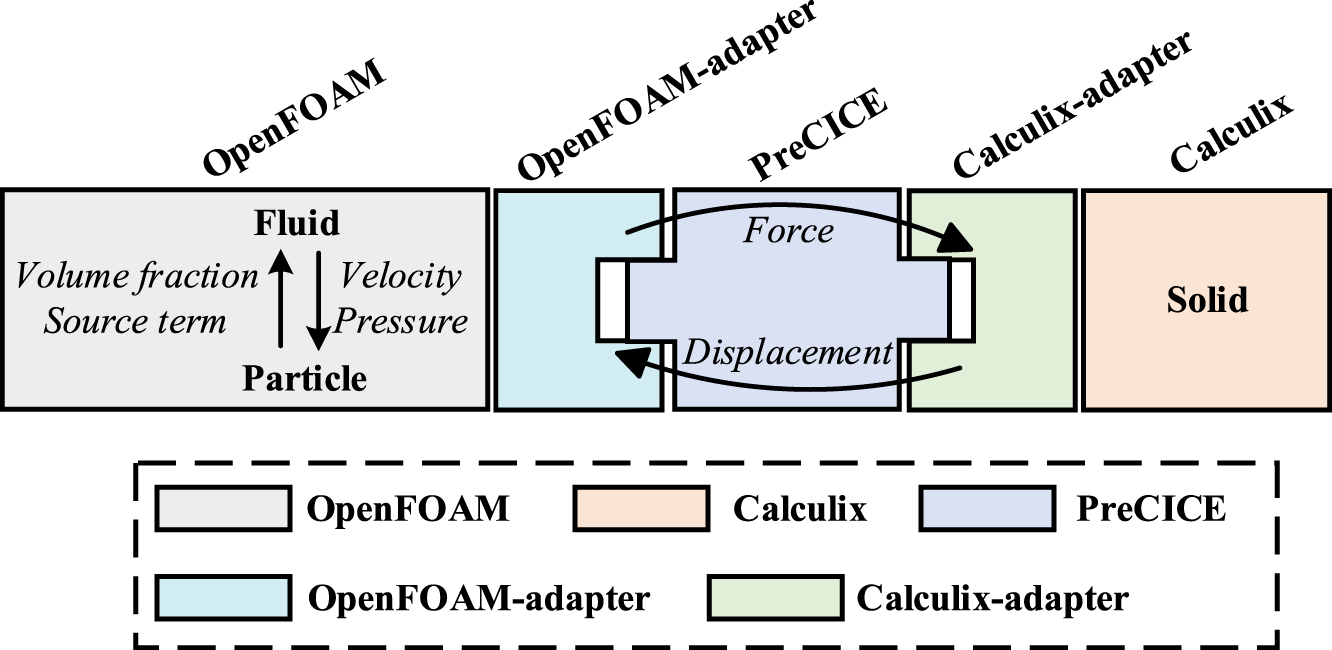
Figure 1: Software architecture of the fluid-particle-structure multiphysics coupling method.
Within the OpenFOAM solver (Left panel of Fig. 1), a bidirectional coupling between the fluid and particle phases is established. The fluid phase provides the macroscopic Velocity and Pressure fields that govern particle motion; reciprocally, the particle phase feedbacks the Volume fraction and momentum Source terms to the fluid governing equations, accounting for the influence of the particle cloud on the flow field.
At the interface between solvers (Middle and Right panels of Fig. 1), PreCICE acts as the coupling middleware handling the data exchange between OpenFOAM and CalculiX. Through the respective adapters, the total Force exerted by both fluids and particles on the structural boundary is mapped to CalculiX to compute deformation. Consequently, the resulting structural Displacement is transferred back to OpenFOAM via PreCICE to update the dynamic mesh. This exchange of Force and Displacement ensures the numerical stability and kinematic compatibility of the multi-physics simulation.
The dynamics of the fluid and particle phases are solved using the MPPICDyMFoam solver of the open-source CFD software OpenFOAM. Its coupling interface is implemented via the OpenFOAM-adapter, which is developed on the basis of the adapter by Chourdakis et al. [48], enabling OpenFOAM to be treated as a black-box solver and efficiently interfaced with PreCICE. The governing equations of the structure are solved using CalculiX, a finite element solver developed by Dhondt [41]. The structural solver coupling interface is realized through the CalculiX-adapter, developed by Benjamin et al. [49], which connects CalculiX as a black-box FEM solver to the PreCICE coupling framework.
For the fluid-particle simulation, OpenFOAM serves as the CFD solver and applies the MPPIC method to capture the interaction between particles and the fluid. OpenFOAM solves macroscopic fluid variables such as pressure and velocity, while simultaneously computing particle volume fractions and momentum source terms to represent the feedback effect of particle assemblies on the flow field. Conversely, fluid motion also influences particle transport and distribution, thereby establishing the bidirectional coupling between the particle and fluid phases.
It should be noted that the proposed multiphysics coupling method adopts a non-intrusive black-box strategy, meaning that the original solver source codes do not need to be modified. Instead, communication between solvers is realized through adapters and PreCICE. This approach not only preserves the independence of different open-source software packages but also significantly enhances the flexibility and extensibility of the multiphysics coupling framework.
Fig. 2 illustrates the multiphysics coupling procedure for FPSI employed in this study. Within each time step, the fluid field, particle field, and structural field are coupled iteratively through sub-iterations. The detailed process is as follows:
(1) At the beginning of each time step, the OpenFOAM-adapter stores the fluid state information and particle positions. For the fluid and particle solvers, the mesh motion equation is first solved to update the mesh movement. Subsequently, particle motion is computed based on the MPPIC method. When solving the particle field, it is necessary to determine whether the iteration corresponds to the initial sub-iteration. If it is the first sub-iteration, the particle forces are evaluated based on the updated flow field, and particle velocities and positions are updated accordingly; otherwise, the particle motion equations are not solved. Finally, the volume fraction and momentum source terms are corrected in the continuity equations and momentum equations, and the Navier–Stokes equations are solved to obtain fluid velocity, pressure, and related variables. Once the fluid and particle solvers are complete, the OpenFOAM-adapter performs interpolation of the forces on the FSI interface using the conservative interpolation method. The structural displacements at the coupling interface are then imposed on the fluid solver as boundary conditions.
(2) At the beginning of each time step, for the structural solver, the structural displacements are obtained by solving the solid dynamics equations. A consistent interpolation method is employed to transfer the interface forces on the FSI boundary, which are then imposed on the solid solver as boundary conditions.
(3) Finally, once the sub-iterations satisfy the convergence criteria, the computation advances to the next time step. If the interface forces and displacements on the fluid-structure coupling boundary do not meet the convergence tolerance, both solvers (fluid-particle solver and structural solver) exchange interface data and repeat the sub-iterations until convergence is achieved.
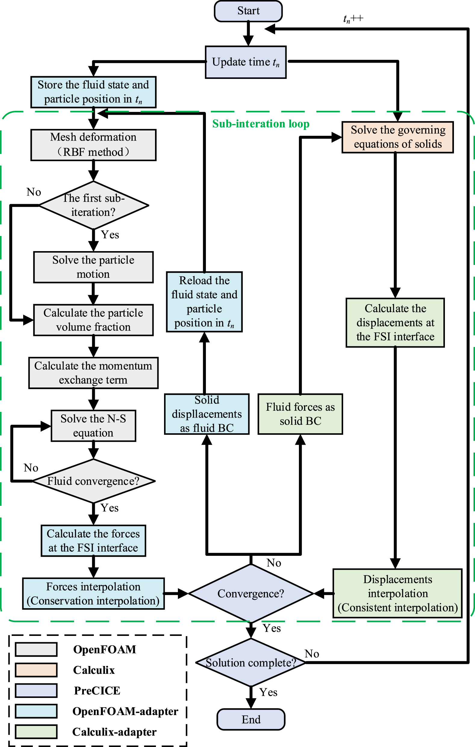
Figure 2: Flowchart of the fluid-particle-structure multiphysics coupling scheme.
In the fluid–particle–structure coupling computation, the adoption of parallel strategies can enhance efficiency. Compared with the serial approach, the parallel method allows the fluid–particle solver and the structural solver to advance simultaneously within the same time step, thereby avoiding complete alternating waits and generally yielding higher computational efficiency [27–29]. Previous studies have shown that the two strategies provide consistent numerical results [27]. It should be noted that the parallel strategy described here differs from the parallel computation within a single solver, and the two concepts should not be conflated.
The proposed multiphysics coupling method realizes direct coupling between fluid and structure and indirect coupling between particles and structure (via fluid feedback), thereby ensuring the rationality of multiphysics interactions and the stability of numerical computations. In this study, the particle–structure interaction is characterized by its indirect nature: when particles collide with the wall, their motion is directly influenced by the structure; however, the feedback from particles to the structure is not transmitted through explicit contact forces; instead, it is conveyed indirectly by altering the fluid parameters at the fluid–structure coupling interface, which are then passed on to the structural domain. Thus, the particle–structure interaction can be regarded as an indirect two-way coupling.
4.1.1 Free Settling of a Spherical Particle in Water
To verify the accuracy and robustness of the fluid-particle coupling model in handling particle sedimentation problems, the classical case of “free settling of a spherical particle in water” [50] is selected as the validation case in this study. This case is widely used for the validation of multiphase flow modeling methods and is suitable for assessing fluid–particle coupling algorithms. By comparing the results with theoretical drag models and previous studies, the numerical simulation accuracy of fluid-particle coupling can be effectively verified.
In this case, a spherical particle with a diameter of dp is released from rest into a water-filled container. The case illustrated is shown in Fig. 3. The fluid density is ρf = 1000 kg/m3, and the kinematic viscosity is vf = 1.0 × 10⁻⁶. The computational domain measures 40dp × 40dp × 200dp, and a structured mesh is employed. The mesh size ratio (Δx/dp) is set to 2, 5, 10, and 50, respectively. The gravitational acceleration is g = 9.81 m/s2, directed along the negative y-axis. The particle density is ρp = 2650 kg/m3, with particle diameters dp of 1, 2, and 5 mm. The initial distance of the particles from the bottom surface is hp = 0.8 m, and the initial velocity of the particles is zero. Driven by gravity, the particle begins to settle and gradually approaches a terminal settling velocity under the combined influence of fluid viscous and inertial drag forces.
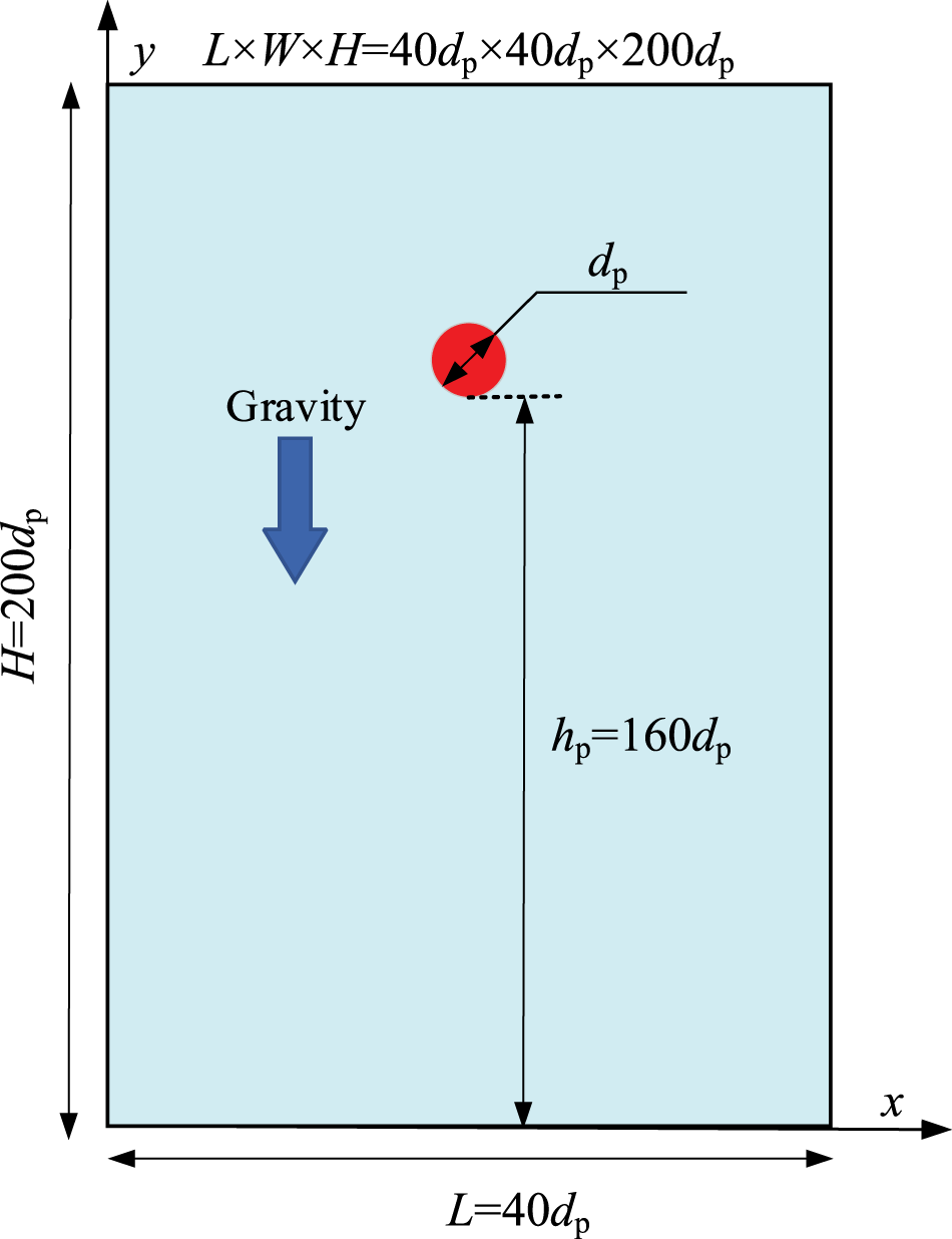
Figure 3: Schematic illustration of a spherical particle freely settling in water.
No-slip boundary conditions are applied to all domain boundaries. The computational domain is sufficiently large to neglect boundary effects on the settling process, ensuring that the single-particle settling behavior can be regarded as free settling in an infinite fluid domain.
To validate the accuracy of the numerical simulation method used in this study, the empirical formula for the free settling velocity of sediment particles proposed by Yang et al. [51] is adopted for comparison. The formula proposed by Yang et al. applies to particle Reynolds numbers 0 < Rep < 2 × 10⁵ and has been shown to agree well with experimental measurements. The terminal settling velocity ut, attained when particles reach a uniform settling state, can be obtained by solving the following equation:
where dp represents the dimensionless particle diameter,
The settling velocities of different particle diameters (dp) and mesh size ratios (Δx/dp) are shown in Fig. 4. It can be observed that the particle motion exhibits typical nonlinear dynamic characteristics: in the initial stage, the particles accelerate downward under the action of net gravity (gravity minus buoyancy). As the speed increases, the fluid resistance significantly increases, and the motion acceleration gradually decreases. When the drag force and buoyancy dynamically balance the gravitational force, the particle reaches a uniform settling stage (terminal velocity state).
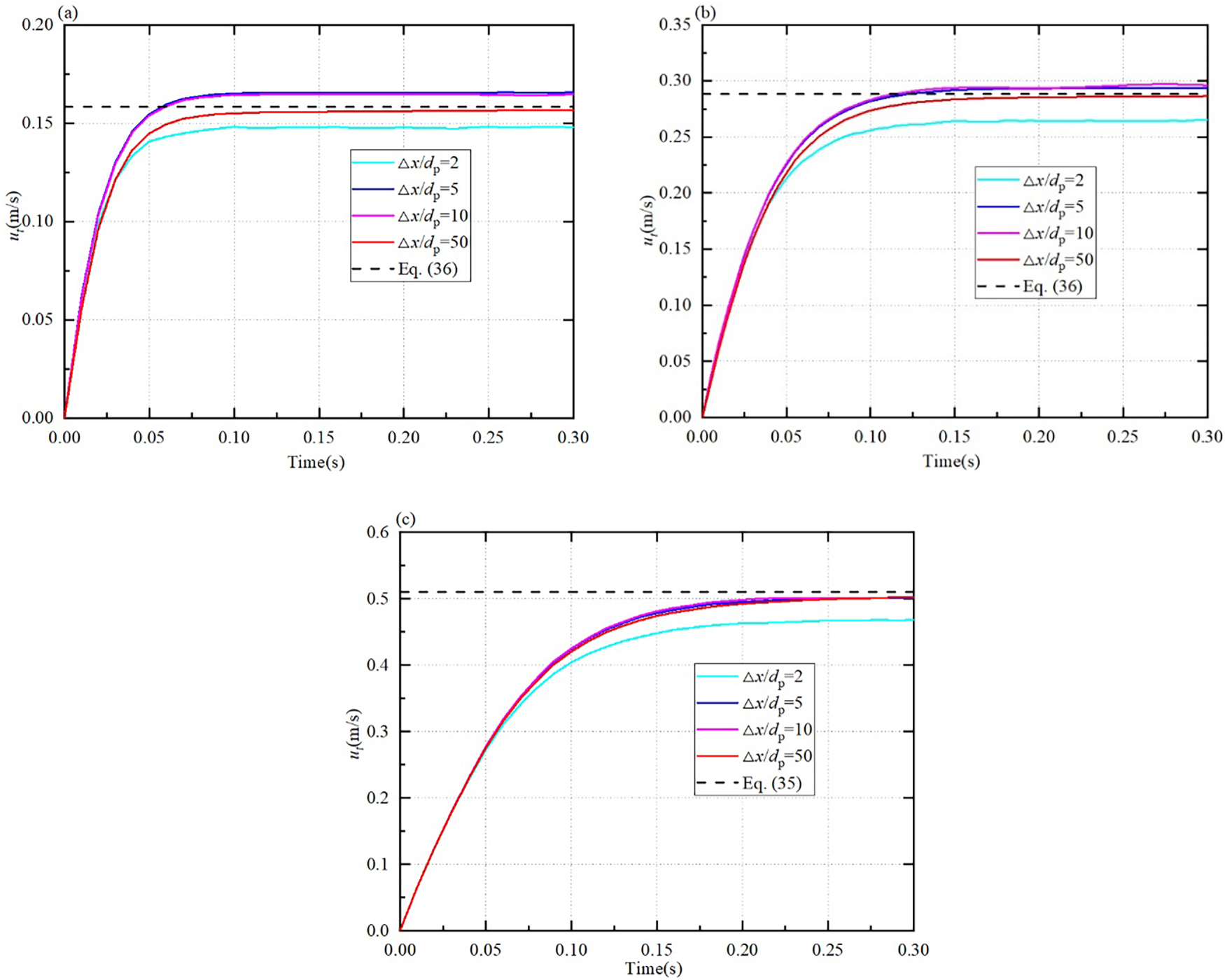
Figure 4: Instantaneous settling velocity of particles with different particle diameters (dp) and grid size ratios (Δx/dp). (a) dp = 1 mm, (b) dp = 2 mm, (c) dp = 5 mm.
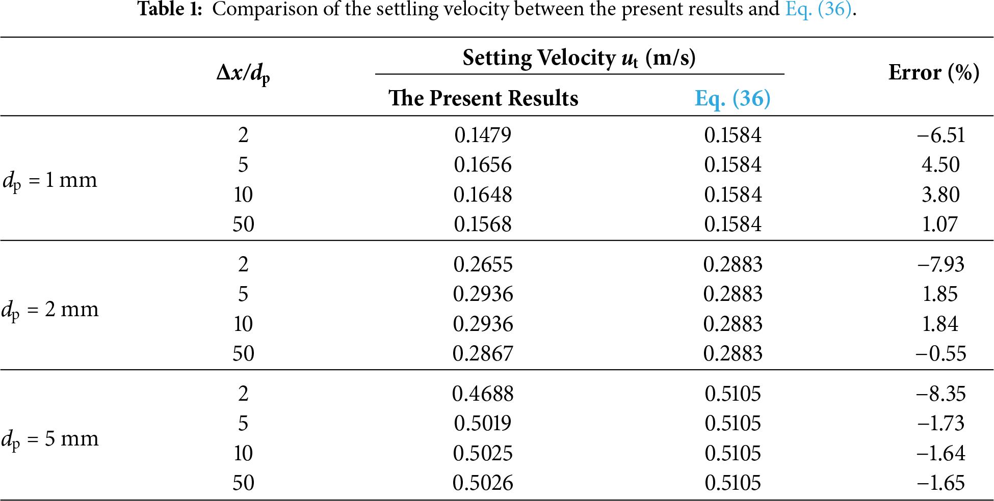
Table 1 presents a comparison between the settling velocities obtained in this study and those predicted by Eq. (36). It can be seen that when Δx/dp = 2, the error in the present results is relatively large, which is attributed to the small mesh size and the resulting discretization errors. When Δx/dp = 5, 10, and 50, the maximum error of the present results is only 4.5%. This indicates that the proposed FPS method can effectively simulate the motion of particles with different diameters.
4.1.2 Free Settling of a Particle Swarm in a Fluid
To verify the accuracy and robustness of the fluid–particle coupling model in handling particle-swarm sedimentation problems, the benchmark sedimentation experiment of Peysson and Guazzelli [52] is adopted. By simulating the free settling of particle swarms with different volume fractions and comparing the particle settling velocity distributions along the horizontal and vertical directions, the reliability of the present fluid–particle coupling model is assessed.
The numerical configuration follows the experimental parameters of Peysson et al. The computational domain spans L × W × H = [0, 0.04 m] × [0, 0.04 m] × [0, 0.5 m], and is filled with fluid of density ρf = 1090 kg/m3 and kinematic viscosity vf = 1.3 × 10⁻³ m2/s, gravity g = 9.81 m/s2 acts in the negative z-direction. A structured hexahedral mesh is used throughout the domain, and all boundaries are smooth walls. The mesh resolution Δx/dp = 3. The particle density ρp = 2530 kg/m3, and the particle diameter is dp = 0.788 mm. At the initial moment, particles are uniformly distributed in the upper region of the domain with an initial volume fraction
According to the observations of Peysson and Guazzelli [52], the free settling of a particle suspension may induce intrinsic convection within the particle swarm, where particles near the sidewalls settle more slowly while those near the center settle faster. By comparing the mean particle settling velocity across different positions in the x-direction, the accuracy of the present numerical method is evaluated.
Following the statistical procedure of Peysson and Guazzelli [52], the computational domain is divided into ten equal segments along the x-direction. Once the settling velocity reaches a statistically steady state, the mean particle velocity in the z-direction for all particles is computed, followed by the mean particle velocities in both the x- and z-directions within each segment. Fig. 5 presents the ratios of the mean settling velocities, together with the experimental data of Peysson et al. The results show that, at a particle volume fraction of 5%, the mean settling velocity in the z-direction is nearly uniform along the x-direction. At 10%, the settling velocity in the central region becomes slightly higher, while that near the walls becomes lower due to interparticle interactions within the swarm. The overall distribution trend agrees well with the experimental observations of Peysson et al., demonstrating that the proposed fluid–particle coupling model accurately captures the settling behavior of particle swarms.
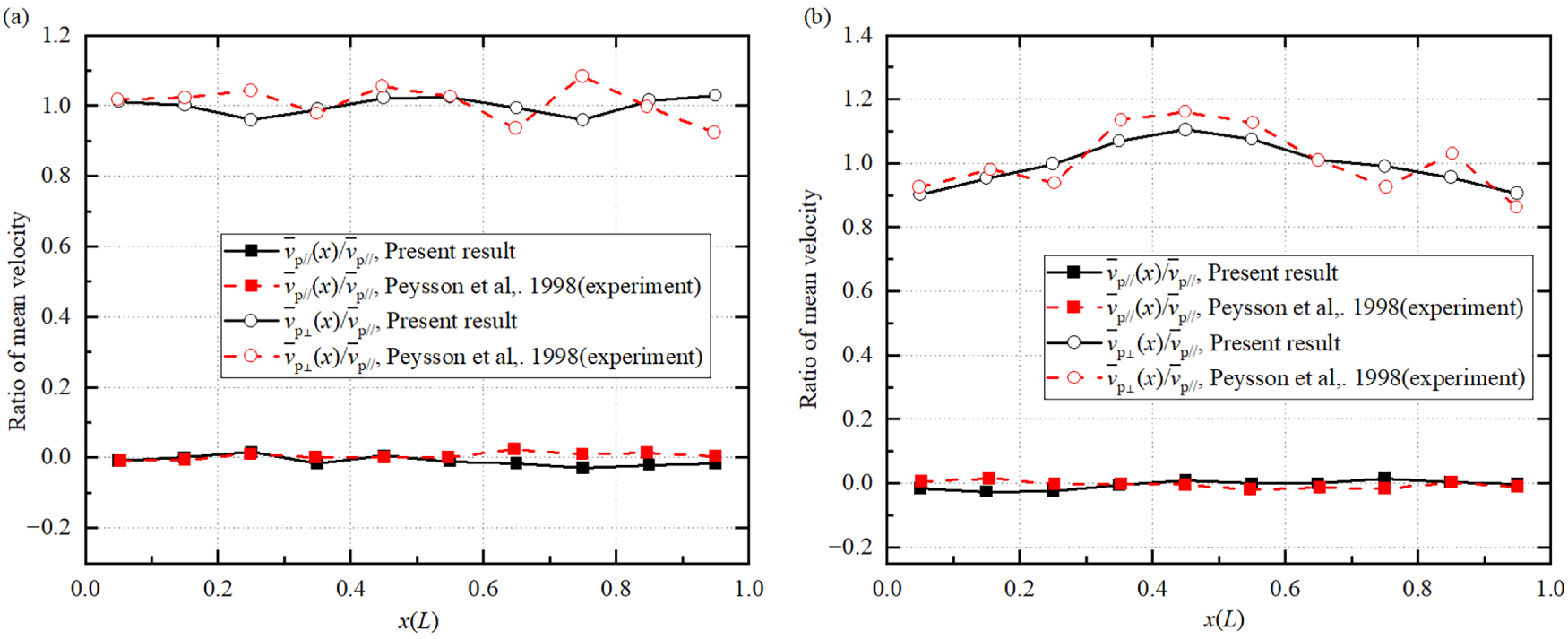
Figure 5: Distribution of the settling velocity of the particle swarm along the x-axis: (a) initial particle swarm volume fraction
To further quantitatively evaluate the agreement between the numerical results and the experimental data, an error analysis was performed on the results presented in Fig. 5. Adopting the statistical method of Peysson et al., the average particle settling velocity ratios within each x-wise section were compared. The relative error between the numerical and experimental results was calculated as Vnum, where Vnum represents the simulated average settling velocity ratio obtained in this study, and Vexp denotes the experimental measurements by Peysson et al.
At an initial particle volume fraction of 5%, as illustrated in Fig. 5a, the average settling velocity in the z-direction exhibits a relatively uniform distribution along the x-direction. The numerical results demonstrate a high degree of consistency with the experimental data. The relative errors of the settling velocity ratios across all sections remain generally low, with a maximum error not exceeding approximately 5%. This indicates that under low volume fraction conditions, where particle-particle interactions are weak and fluid dynamics dominate particle motion, the established fluid-particle coupling model accurately captures the macroscopic kinematic characteristics of the particle cloud during free settling.
When the initial particle volume fraction is increased to 10%, as depicted in Fig. 5b, the internal interactions within the particle cloud intensify. The free settling process induces distinct internal convection structures, resulting in slightly faster settling velocities near the center of the computational domain and relatively reduced velocities near the wall regions. The numerical simulation results successfully reproduce this non-uniform distribution trend observed in the experiments. Although the relative error increases slightly in local regions (particularly near the center), the overall error remains controlled within approximately 8%. This demonstrates that the proposed model retains good stability and predictive capability even under higher volume fraction conditions.
It should be noted that the slight increase in error under high volume fraction conditions is primarily attributed to the intensification of particle-particle interactions, particle-wall effects, and local non-uniform flow structures. These factors increase the sensitivity of particle motion and place higher demands on the resolution capability of the numerical model. Nevertheless, the numerical results remain consistent with the experimental data in terms of overall trends, positions of extrema, and distribution patterns. This indicates that the established fluid-particle coupling model not only accurately predicts the average settling velocity of the particle cloud but also reasonably reflects the spatial non-uniformity induced by the evolution of internal structures during sedimentation.
In summary, the error analysis further demonstrates that the proposed fluid-particle coupling model possesses high computational accuracy and good robustness across different particle volume fractions, enabling reliable simulation of the free settling behavior of particle clouds in fluids.
4.2 FSI Benchmark Case: Coupled Vibration of the Flexible Beam behind the Cylinder
This benchmark case is one of the classical FSI benchmarks proposed by Turek and Hron [53]. A schematic of the case is shown in Fig. 6. The simulated object is a fixed cylinder with the flexible beam attached to its rear end, which undergoes periodic vibration under the action of the incoming flow. The dynamic response in this case mainly arises from the interaction between the inflow and the flexible beam. The separated vortex system formed in the wake of the beam excites its vibration, leading to the occurrence of a Kármán vortex street.
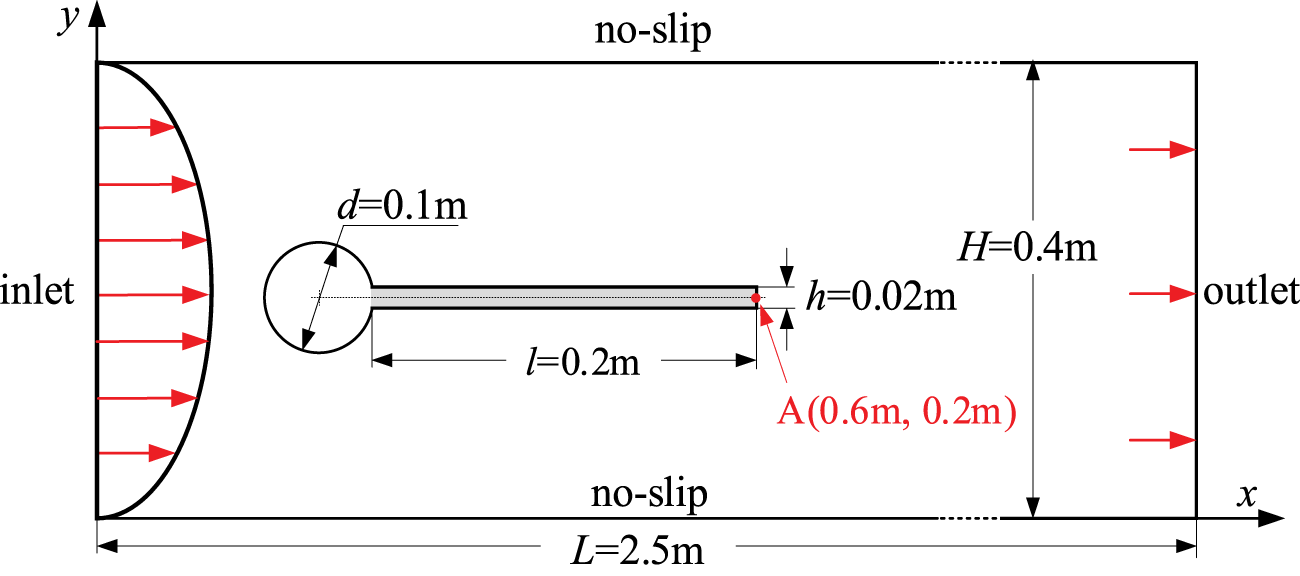
Figure 6: Schematic diagram of vortex-induced vibration of the flexible beam behind the cylinder.
In this case, the computational domain contains a fixed cylinder. The length and width of the domain are L = 2.5 m and H = 0.4 m, respectively. The cylinder has a diameter of d = 0.1 m, with its center located at (0.3, 0.2 m). The fluid density is ρf = 1 × 10³ kg/m3, and the kinematic viscosity is vf = 0.001 m2/s. On the right side of the flow field is the pressure outlet boundary condition. The upper and lower boundaries are subjected to no-slip boundary conditions, and the left side is the velocity inlet boundary condition, where the inlet velocity uf-inlet follows a parabolic profile that gradually increases with time, as defined in Eq. (41). The mean inlet velocity is ua = 1 m/s. The Reynolds number is Re = Ufd/vf = 100. The flexible beam has a length of l = 0.2 m and a width of h = 0.02 m. Its left end is rigidly attached to the cylinder, while the right end is free. The beam has a Poisson’s ratio of ν = 0.4, a density of ρs = 1.0 × 10⁴ kg/m3, and a Young’s modulus of E = 1.4 MPa. These parameters ensure that the excitation frequency induced by the inflow is close to the first natural frequency of the structure, thereby triggering a pronounced resonance response.
The fluid mesh used in the computation consists of multi-block structured grids, with a total of 38,489 structured grids. The structural domain is discretized with 200 C3D20 second-order solid elements. Figs. 7 and 8 show the displacements of point A in the x-direction and y-direction, respectively. It can be observed that the amplitude of the flexible beam increases gradually, and after 10 s, the beam begins to oscillate periodically.
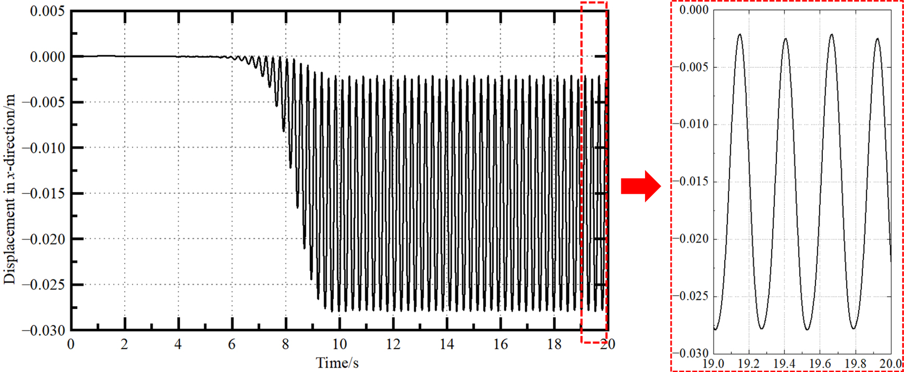
Figure 7: The displacement of point A in the x direction.
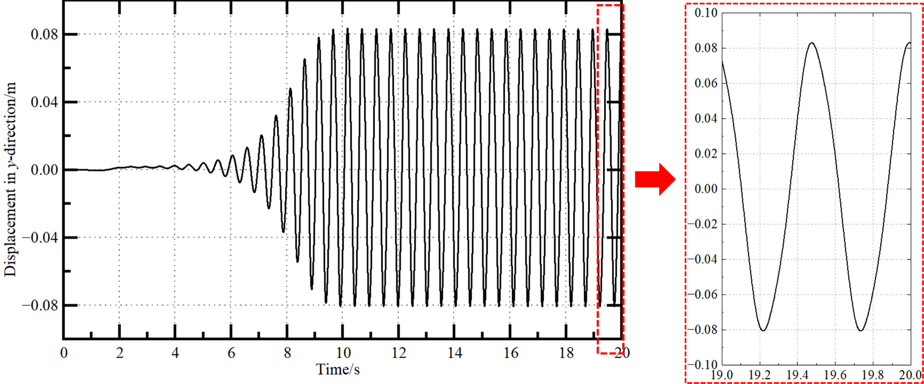
Figure 8: The displacement of point A in the y direction.
To more intuitively illustrate the coupling characteristics between the flow field and the structural response in the FSI process, five representative time instants from the benchmark case are selected for comparative analysis of the fluid velocity contours and structural displacement contours, as shown in Fig. 9. The results show that, at each instant, the variations in the velocity field are closely correlated with the oscillatory behavior of the flexible beam. As the fluid flows past the beam, alternating vortex streets are generated, inducing significant transverse vibrations of the structure.
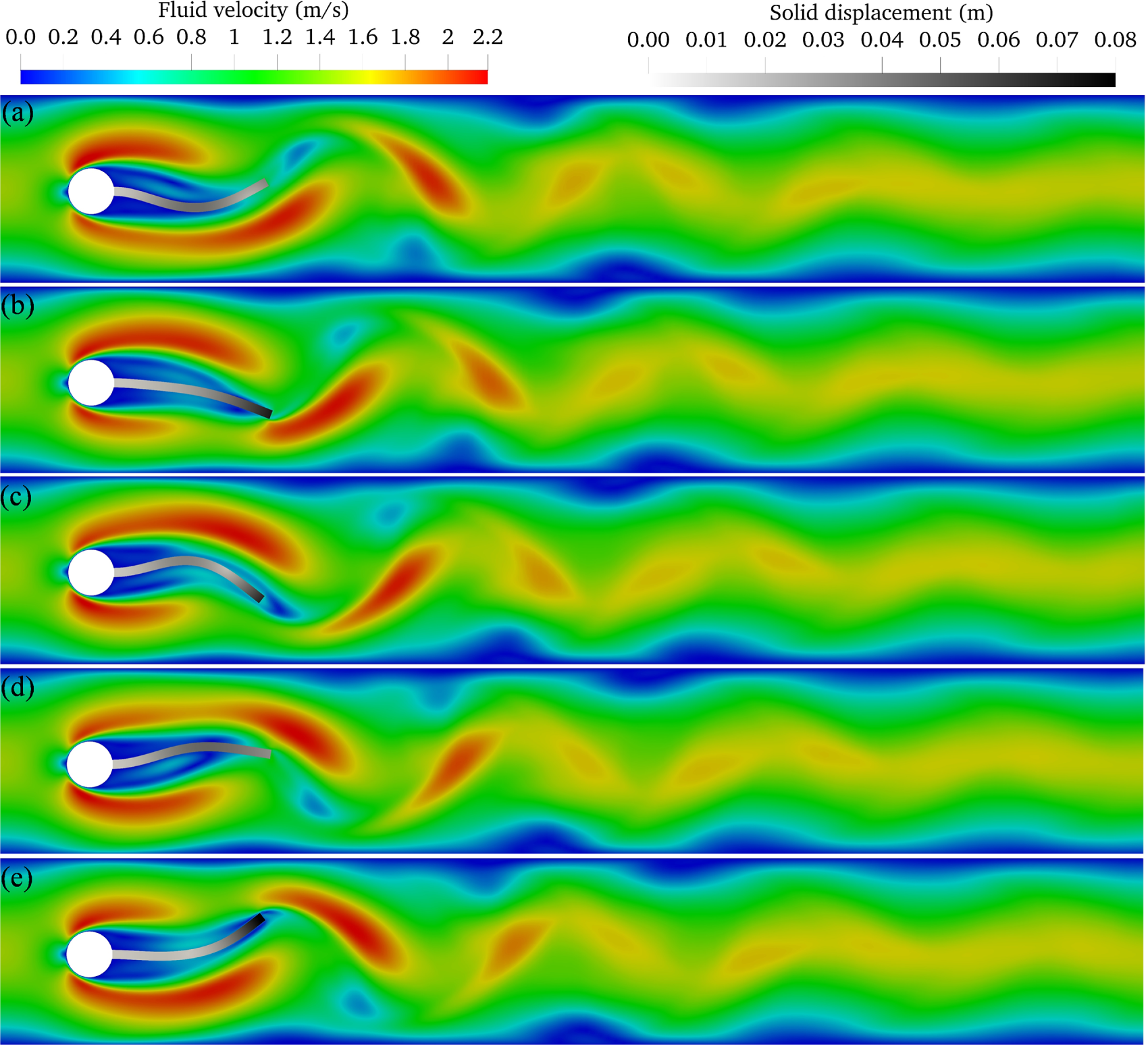
Figure 9: Fluid velocity contours and solid displacement contours at five typical time instants. (a) Time = 19.6 s, (b) Time = 19.7 s, (c) Time = 19.8 s, (d) Time = 19.9 s, (e) Time = 20.0 s.
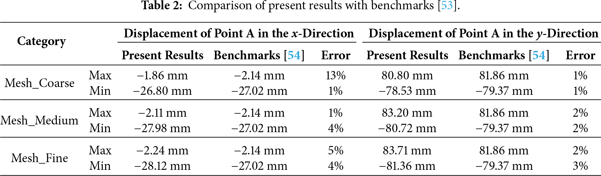
To quantitatively validate the numerical simulation results, the displacements of point A in both the x- and y-directions were compared with the benchmark data [53]. In addition, to examine the mesh and time-step independence of the solution, three sets of simulations were performed using different mesh resolutions and time steps. The coarse mesh consists of 20,969 structural grid nodes and 100 C3D20 solid elements; the medium mesh corresponds to the computational mesh used in the main results and contains 38,489 structural grid nodes and 200 C3D20 second-order solid elements; the fine mesh contains 45,903 structural grid nodes and 300 C3D20 solid elements. The time steps associated with the coarse, medium, and fine meshes were 0.002, 0.001, and 0.0005 s, respectively. The results obtained with the three different spatial and temporal resolutions are summarized in Table 2, from which it can be observed that the numerical predictions of this study exhibit good agreement with the benchmark solution.
4.3 PSI Benchmark Case: Collision Process between a Spherical Particle and the Ground
To verify the accuracy of the proposed numerical method in simulating particle–ground collisions in a viscous fluid, a systematic comparison was conducted with the classical experimental results of Joseph et al. [54]. In their study, Joseph et al. experimentally investigated the dynamics of a single particle colliding with the solid ground in the viscous fluid. At the initial moment of the experiment, the particle was assigned an initial velocity in the fluid. Driven by this velocity, the particle began to descend, during which the fluid imposed a resisting effect, causing the particle velocity to gradually decrease until it impacted the solid wall. A high-speed camera was employed to record the particle motion throughout the experiment, thereby capturing the velocity changes before and after the collision. It should be noted that in the experiment, the effect of gravity on the particle was eliminated by suspending it with a string.
The schematic of the computational domain for the particle-ground collision is shown in Fig. 10. In this study, the computational domain is defined as a three-dimensional rectangular region, designed to simulate the vertical motion of a single particle in a viscous fluid and its subsequent collision with a fixed lower wall. The domain height is set to 40 times the particle diameter to provide sufficient flow development space, while the width is also set to 40 times the particle diameter to avoid boundary interference. Initially, the particle is positioned at the center of the domain, with a distance of hp = 13.365 mm, above the lower wall. The particle diameter is dp = 0.635 cm, and the particle density is ρp = 2540 kg/m3. The initial velocity is up-initial = 12.5 cm/s. The normal restitution coefficient between the particle and the lower wall surface is en = 0.8, while the tangential restitution coefficient is et = 1. The effect of gravity on the particle is neglected, so the particle is influenced only by the viscous drag and inertial forces of the fluid. The fluid density is ρf = 1000 kg/m3, and the kinematic viscosity is vf = 1.0 × 10⁻⁶ m2/s. The mesh size Δx is set to 10 and 20 times the particle diameter, respectively. For the sake of comparison, the simulation parameters in this benchmark case are aligned with the experimental conditions of Joseph et al. [54] and the numerical setup of Feng et al. [55].
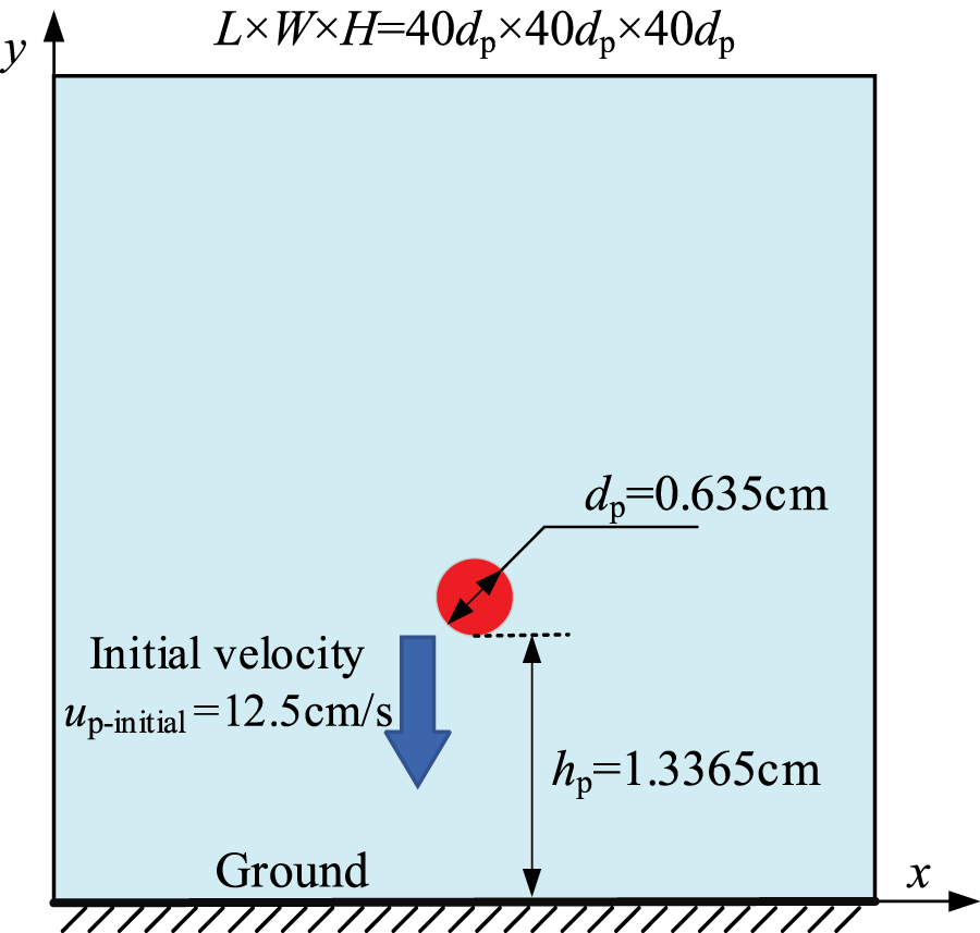
Figure 10: Schematic illustration of the computational domain for a spherical particle colliding with the ground.
The physical boundary conditions are specified as follows: the lower boundary is modeled as a fixed ground with the no-slip condition to simulate the realistic particle-ground collision process; the upper boundary is defined as an open boundary or a free-slip boundary to minimize boundary effects; while the lateral boundaries are set as free-slip boundaries to ensure flow field stability. Between the particle surface and the fluid, fluid-particle coupling boundary conditions are imposed to capture the dynamic response of particles in the fluid and their contact behavior with the ground.
Fig. 11 presents the velocity profiles before and after particle-ground collisions for cases with grid-to-particle diameter ratios (Δx/dp) of 20 and 10. It can be observed that as the particle approaches the wall, its velocity gradually decreases due to the viscous drag of the fluid. At the moment of collision, the particle velocity undergoes a sharp change, transitioning from an approaching state to a rebounding state. After moving away from the wall, the particle again experiences viscous resistance from the fluid, leading to gradual deceleration. For validation, the present results are compared with numerical predictions [55] and experimental measurements [54], showing good agreement. This confirms the reliability of the proposed method in capturing the particle-ground collision dynamics under the influence of viscous fluid effects.
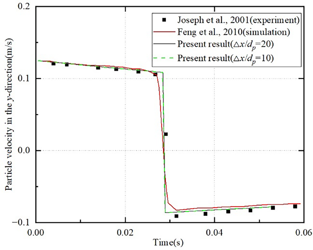
Figure 11: Particle approaching velocity and rebound velocity near the ground [54,55].
5 Analysis of Examples: Deformation of the Flexible Plate in the Solid-Liquid Two-Channel Flow
This case study aims to investigate the fluid-particle-structure coupled dynamics of an elastic structure subjected to a fluid-particle mixture, and to demonstrate the capability of the present numerical simulation method in handling multiphysics interactions involving fluid, particles, and large-deformation structures. By introducing a solid–liquid multiphase MPPIC model in a two-dimensional channel, the impact of particle-laden flow on an elastic plate and the resulting flow-induced vibrations are simulated. Introduce different particle flow rates to analyze the coupled behavior of the fluid, particles, and structure.
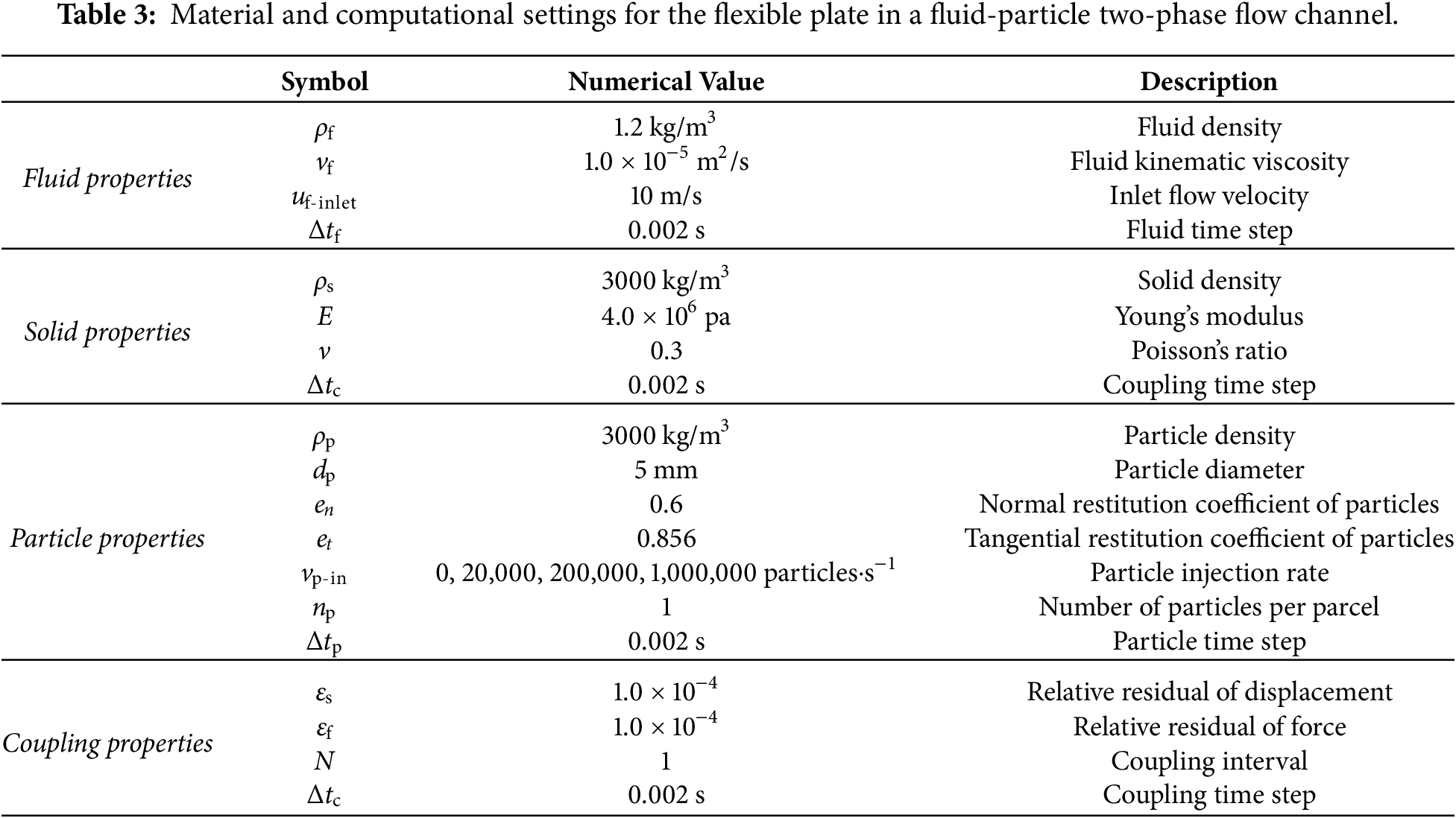
The schematic of the case is shown in Fig. 12. The computational domain is a two-dimensional rectangular channel with a length of L = 6 m in the x-direction and a height of H = 4 m in the y-direction. An elastic upright plate of length l = 1 m (along the y-direction) and thickness h = 0.1 m (along the x-direction) is fixed at the center of the channel bottom. The plate is rigidly attached to the bottom wall and can undergo elastic deformation under fluid and particle loads. The left boundary is set as a constant-velocity inlet, with the flow direction in the x direction. The inlet fluid velocity is uf-inlet = 10 m/s, carrying a uniformly distributed fluid-particle mixture with particle velocity up-inlet = 0.6 m/s. The right boundary is treated as a pressure outlet. The top and bottom of the channel, as well as the elastic plate surface, are subjected to no-slip conditions, allowing momentum and energy exchange between the fluid, particles, and structure. Except for the inlet and outlet, collisions between particles and walls are considered at all boundaries. Gravity effects are included for both fluid and particles, acting in the negative y-direction. The material properties of the fluid, particles, and structure, along with computational settings, are summarized in Table 3.
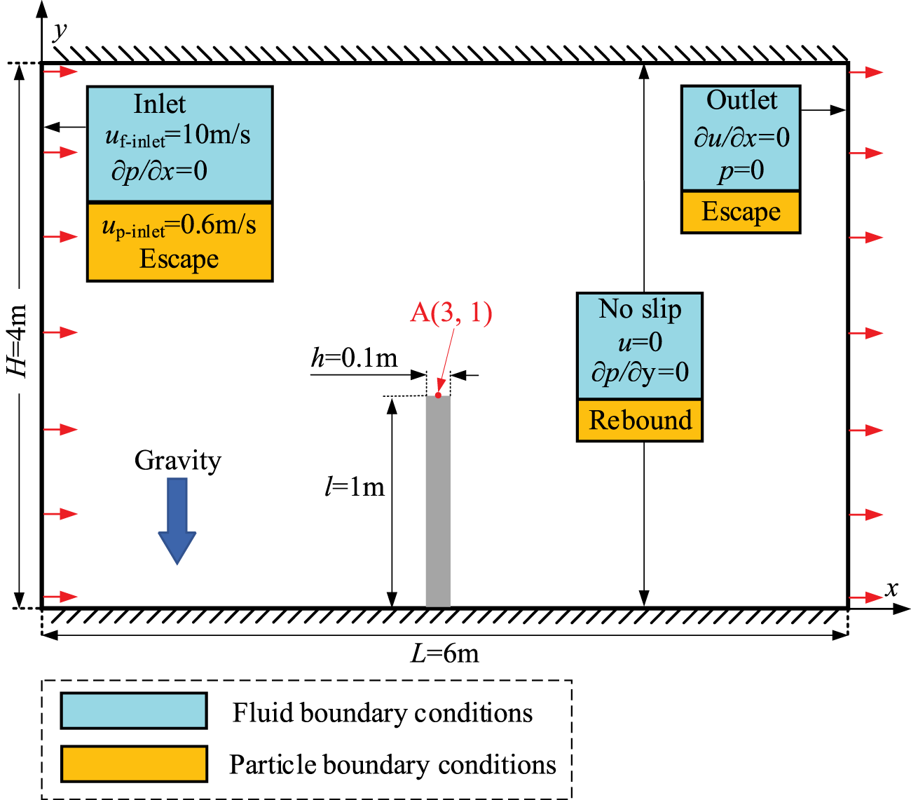
Figure 12: Schematic of a flexible plate deforming in a fluid–particle channel flow.
To evaluate the sensitivity of the numerical results to mesh resolution and time step size, three cases with different combinations of mesh density and time step were conducted. The mesh configurations and time steps for the three cases are summarized in Table 4. Specifically, three levels of mesh resolution were considered: the coarse mesh consists of 120 fluid cells and 100 C3D8I solid elements; the medium mesh consists of 244 fluid cells and 200 C3D8I solid elements; and the fine mesh consists of 400 fluid cells and 300 C3D8I solid elements. The corresponding time steps were 0.002 s, 0.001 s, and 0.0005 s, respectively. Fig. 13 presents the results obtained with these three mesh–time step combinations. It can be seen that the medium mesh with a time step of 0.001 s provides a converged and accurate numerical solution. Therefore, this mesh and time step configuration is adopted for all subsequent simulations.
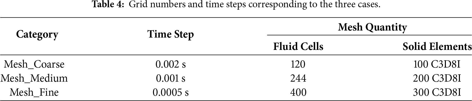
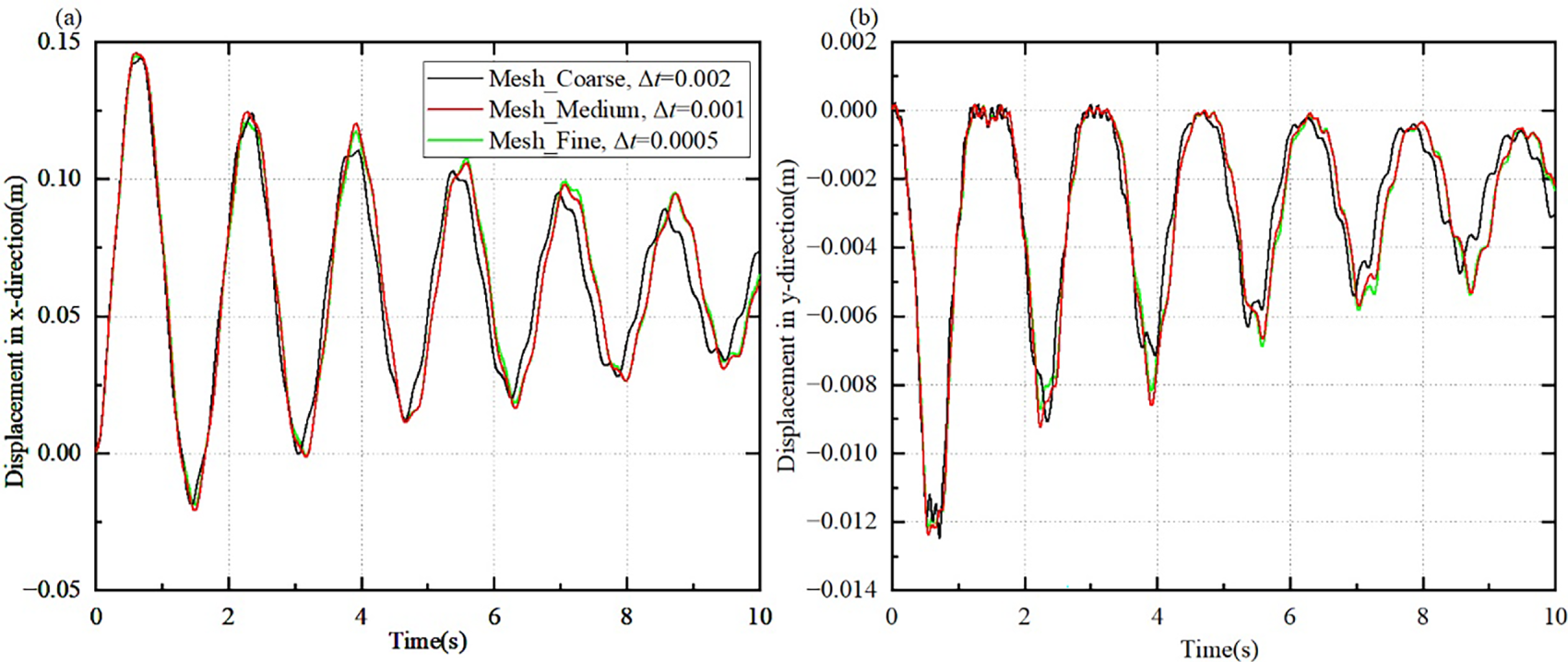
Figure 13: The displacement of point A in the (a) x- and (b) y-directions for three different cases.
Fig. 14 (Multimedia available online) shows the fluid velocity contours, particle velocity distribution, and displacement contours for a particle injection rate of vp-in = 20,000 particles·s−1. The fluid velocity contours illustrate the velocity distribution of the flow field: due to the presence of the flexible plate, a local high-velocity region forms near the plate tip, while flow separation is observed in the downstream region. The displacement contours of the solid reveal the deformation of the flexible plate under the combined action of the fluid and particles. The plate primarily oscillates in the streamwise direction, with the maximum displacement occurring at the tip, whereas the displacement at the root remains relatively small. The particle velocity field reflects the motion characteristics of particles within the channel. Upon entering the flow domain, particles undergo free fall under gravity until colliding with the bottom wall for the first time. Subsequently, driven by the fluid flow and plate oscillations, the particles are carried downstream and collide with the tip surface of the flexible plate. During the collisions, the particle velocity and trajectory undergo significant changes, exhibiting elastic rebound and flow-induced deflection. Eventually, the particles are transported out of the channel.
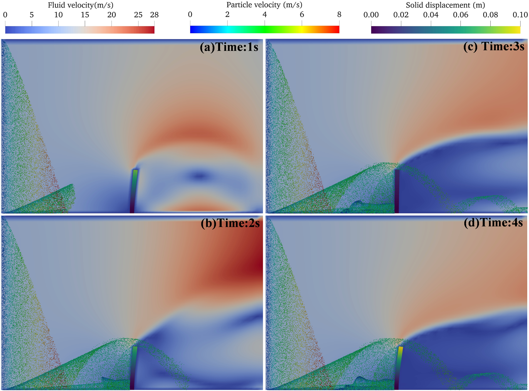
Figure 14: Deformation process of the flexible plate when a liquid-particle flow passes through the channel. The particle injection rate vp-in = 20,000 particles·s−1. Note: For visualization purposes, the particle diameter is magnified by a factor of two. (Multimedia available online).
The oscillation amplitude of the flexible plate results from the combined action of the fluid and particles. Although the present numerical method neglects the direct collision force of particles on the structure, the particles exert resistance and propulsion effects on the fluid. This obstructive/pushing behavior is specifically manifested in the fluid volume fraction
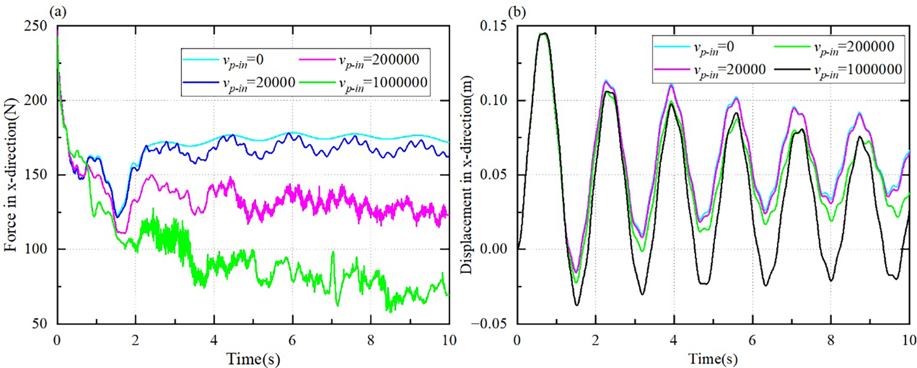
Figure 15: (a) x-direction force on the flexible plate and (b) x-direction displacement of the apex under different particle injection rates.
This case study enables a systematic analysis of the influence of particle injection rate on the vibration characteristics of the elastic plate. Although the case has not been experimentally validated, the results confirm the processing capability of the proposed multiphysics numerical model in handling the coupled processes of fluid, particles, and large-deformation structures. The model applies to investigations of FPSI and provides valuable insights for research in areas such as flow-induced vibrations, particle-laden flow load assessment, and the optimization of transport systems.
6 Applicability of the Proposed Multiphysics Coupling Model
The multi physics implicit coupling model constructed in this study is based on CFD, MPPIC, and FEM methods, and numerical simulation of FPSI is achieved through a partitioned non-invasive coupling framework of OpenFOAM-CalculiX-preCICE. Based on the aforementioned mathematical model, coupling strategy, and limitations, the applicability of this model mainly includes the following aspects:
(1) Suitable for particle flow problems ranging from dilute phase to medium volume fraction. The MPPIC method can reasonably simulate the particle particle interaction in dilute and medium density particle groups, and its collision and friction effects are characterized by collision stress without the need to analyze the real particle contact process. Therefore, this model is applicable to typical scenarios such as sediment transport, pneumatic conveying, suspended particles in the ocean and environment.
(2) Suitable for flexible deformation structures that can withstand fluid and particle loads. The structural field adopts nonlinear finite element method, which can capture large deformations caused by geometric nonlinearity. Therefore, this model is suitable for analyzing the force and dynamic behavior of thin plates, thin films, flexible beams, biomimetic flexible fins, seagrass like flexible structures, etc. in particle flow, especially for structural materials that mainly undergo elastic deformation.
(3) Suitable for coupled systems where particle structure interactions are indirectly transmitted through fluids. This study did not consider the direct contact between particles and structures, so the model is applicable to problems where particles mainly affect structures by changing the flow field load, rather than situations where particles directly impact or erode. Typical applications include suspended sand changing hydrodynamic loads to affect structural deformation, and sand and dust suspension induced by flexible deformation of helicopter rotors in desert environments.
In summary, the multi physics field coupling model proposed in this study provides an efficient, stable, and high fidelity numerical tool for analyzing the dynamic behavior of flexible structures in granular flows. If the particle structure direct contact mechanics model is further introduced in the future, it will significantly expand the application scope of this model.
In this work, a multiphysics implicit coupling method based on CFD, MPPIC, and FEM is proposed. The method is implemented within a partitioned, non-intrusive coupling framework built on the open-source software OpenFOAM, CalculiX, and preCICE, enabling the numerical simulation of FPSI with large structural deformations. The main conclusions are as follows:
(1) The developed multiphysics coupling approach enables parallel iterative solutions of the fluid, particle, and structural fields while ensuring numerical stability. The fluid field is solved using OpenFOAM for the incompressible Navier-Stokes equations, combined with the RBF dynamic mesh technique to effectively address mesh distortion induced by structural motion. The particle phase is modeled using the MPPIC method, where the Liouville equation is adopted to describe the particle distribution function, the momentum exchange model is combined to describe the interaction between particles and fluid, and collision stresses represent particle-particle interactions. The structural field is solved using the FEM, accurately capturing large deformations resulting from geometric nonlinearity. Results demonstrate that the proposed method can stably and accurately simulate FPSI coupling.
(2) The numerical results reveal the complex dynamics among the fluid, particles, and structure. Structural deformation significantly alters the local flow distribution, thereby indirectly affecting particle transport and accumulation. Meanwhile, particle deposition and motion influence the structure through the fluid, modifying its load conditions and deformation amplitude. It should be noted that in this study, the particle–structure interaction is not directly coupled, but mediated through the fluid. This is of great significance for understanding the dynamic response of flexible structures in particle flow environments.
(3) This study provides an efficient and reliable numerical tool for investigating the dynamics of flexible structures under particle-laden flows. The proposed approach can be applied to research on flow-induced vibrations, particle-laden flow load assessment, and transport system optimization. Furthermore, the implicit multiphysics coupling strategy presented here offers a valuable reference for the numerical modeling of other complex multiphase systems.
It should be noted that this study still has certain limitations. First, the MPPIC method introduces simplifications in modeling inter-particle contact forces, making it difficult to fully capture the collision and frictional behaviors observed in real granular systems. Second, the particle–structure interaction is modeled through an indirect coupling strategy, and the direct mechanical contact between particles and the structure is not incorporated into the current framework. In addition, the body-fitted mesh approach in the fluid–structure coupling may struggle to maintain mesh quality when boundary points undergo large-amplitude motions or rotations. Finally, due to the high computational cost associated with strongly coupled multiphysics simulations, the proposed method remains constrained by resource and efficiency limitations when applied to large-scale three-dimensional problems.
Acknowledgement: Not applicable.
Funding Statement: This work was supported in part by the Mining Hydraulic Technology and Equipment Engineering Research Center, Liaoning Technical University, Fuxin, China (Grant No. MHTE23-R04), the Fundamental Research Funds for the Central Universities (ID N25BSS068).
Author Contributions: The authors confirm contribution to the paper as follows: Conceptualization, Xiangxiang Wang and Hualong Xie; methodology, Xiangxiang Wang; software, Xiangxiang Wang and Yue Yu; validation, Xiangxiang Wang, Hualong Xie, and Yue Yu; formal analysis, Xiangxiang Wang and Min Li; investigation, Xiangxiang Wang and Yubin Wang; resources, Hualong Xie and Fei Xing; data curation, Xiangxiang Wang and Yue Yu; writing—original draft preparation, Xiangxiang Wang; writing—review and editing, Hualong Xie, Yue Yu, and Min Li; visualization, Xiangxiang Wang and Yubin Wang; supervision, Hualong Xie; project administration, Hualong Xie; funding acquisition, Hualong Xie. All authors reviewed and approved the final version of the manuscript.
Availability of Data and Materials: The data that support the findings of this study are available from the corresponding author, Hualong Xie, upon reasonable request.
Ethics Approval: Not applicable. This study did not involve human participants or animal experiments.
Conflicts of Interest: The authors declare no conflicts of interest.
Supplementary Materials: The supplementary material is available online at https://www.techscience.com/doi/10.32604/cmes.2026.075270/s1, and include multimedia content associated with Fig. 13.
Nomenclature
| English | symbols |
| Ap | Particle acceleration |
| C | Elasticity tensor |
| Cd | Wen-Yu drag coefficient |
| D1 | Wen-Yu drag model |
| D2 | Ergun drag model |
| df | Displacement vector on the fluid interface |
| Dp | Drag coefficient |
| dp | Particle diameter |
| Dimensionless particle diameter | |
| ds | Solid displacement vector |
| Interface displacement at the (i − 1)-th sub-iteration | |
| Under-relaxed displacement | |
| Displacement at the i-th iteration | |
| E | Green-Lagrange strain tensor |
| E | Young’s modulus |
| en | Normal restitution coefficient of particles |
| et | Tangential restitution coefficient of particles |
| F | Momentum coupling term between particles and fluid |
| f | Particle distribution function |
| F | Computation of force from displacement at the FSI interface |
| fb | Solid body force |
| ff | Force vector on the fluid interface |
| fs | Force vector on the solid interface |
| Interface force at the (i−1)-th sub-iteration | |
| Under-relaxed force | |
| Force at the i-th iteration | |
| g | Gravitational acceleration |
| H | Computational domain height |
| h | Plate thickness |
| hp | Distance between particle and bottom wall |
| I | Fluid unit stress tensor |
| L | Computational domain length |
| l | Plate length |
| mp | Particle mass |
| N | Coupling interval |
| Nf | Number of coupling interface nodes in the fluid domain |
| np | Number of particles per parcel |
| Ns | Number of coupling interface nodes in the solid domain |
| p | Fluid pressure |
| r | Euclidean distance from a fluid mesh point to a coupling interface node |
| Re | Fluid Reynolds number |
| Rep | Particle Reynolds number |
| rp | Particle radius |
| Displacement residual at the i-th sub-iteration | |
| Force residual at the i-th sub-iteration | |
| S | Second Piola–Kirchhoff stress tensor |
| S | Computation of displacement from force at the FSI interface |
| t | Time |
| u | Displacement of an arbitrary mesh node |
| ua | Inlet average velocity |
| uf | Fluid velocity |
| uf-inlet | Inlet flow velocity |
| Post-collision wall-normal velocity of particles | |
| Pre-collision wall-normal velocity of particles | |
| Post-collision wall-tangential velocity of particles | |
| Pre-collision wall-tangential velocity of particles | |
| up | Particle velocity |
| up-initial | Initial particle velocity |
| up-inlet | Inlet particle velocity |
| Particle velocity at the next time step | |
| Particle velocity at the current time step | |
| Fluid velocity interpolated at the particle location | |
| ut | Terminal settling velocity of particles |
| v | Poisson’s ratio |
| vf | Fluid kinematic viscosity |
| Vp | Particle volume |
| vp-in | Particle injection rate |
| w | Under-relaxation factor |
| W | Computational domain width |
| x | Coordinate value of an arbitrary point in the fluid mesh coordinate system |
| xp | Particle position |
| Xp | Inter-particle collision force |
| Parcel position at the next time step | |
| Parcel position at the current time step | |
| Displacement at the FSI interface node | |
| Greek symbols | |
| β | Empirical parameter |
| Fluid stress tensor | |
| Effective fluid viscosity | |
| Dynamic mesh basis function | |
| Particle stress | |
| Particle volume fraction | |
| Fluid volume fraction | |
| Maximum random packing particle volume fraction | |
| Pressure gradient at the particle location | |
| Stress gradient at the particle location | |
| Δx | Fluid mesh size |
| Δtc | Coupling time step |
| Δtf | Fluid time step |
| Δtp | Particle time step |
| εf | Relative residual of force |
| εs | Relative residual of displacement |
| λ | Lamé constants |
| μ | Dynamic viscosity coefficient |
| μ | Lamé constants |
| μf | Fluid dynamic viscosity |
| μt | Turbulent viscosity coefficient |
| ρp | Particle density |
| ρs | Solid density |
| ρf | Fluid density |
References
1. Liu C, Yu Z, Zhao S. A coupled SPH-DEM-FEM model for fluid-particle-structure interaction and a case study of Wenjia gully debris flow impact estimation. Landslides. 2021;18(7):2403–25. doi:10.1007/s10346-021-01640-6. [Google Scholar] [CrossRef]
2. Wang L, Zhou G, Wang X, Xiong Q, Ge W. Direct numerical simulation of particle-fluid systems by combining time-driven hard-sphere model and lattice Boltzmann method. Particuology. 2010;8(4):379–82. doi:10.1016/j.partic.2010.07.003. [Google Scholar] [CrossRef]
3. Bazilevskii AV, Koroteev DA, Rozhkov AN, Skobeleva AA. Sedimentation of particles in shear flows of viscoelastic fluids. Fluid Dyn. 2010;45(4):626–37. doi:10.1134/s0015462810040125. [Google Scholar] [CrossRef]
4. Hou T, Wei X, Iqbal AA, Yang X, Wang J, Ren Y, et al. Advances in biomedical fluid-structure interaction: methodologies and applications from an interfacing perspective. Phys Fluids. 2024;36(2):021301. doi:10.1063/5.0189218. [Google Scholar] [CrossRef]
5. Zhang T, Ding HH, Su Y, Chen H. Modal analysis of multi-span pipes conveying fluid based on three different FSI methods. Adv Mater Res. 2012;594-597:2525–8. doi:10.4028/www.scientific.net/amr.594-597.2525. [Google Scholar] [CrossRef]
6. Qin J, Liao F, Dong G, Yang X. Parallelization strategies for resolved simulations of fluid-structure-particle interactions. Appl Math Mech Engl Ed. 2024;45(5):857–72. doi:10.1007/s10483-024-3115-7. [Google Scholar] [CrossRef]
7. Hoorijani H, Esgandari B, Zarghami R, Sotudeh-Gharebagh R, Mostoufi N. CFD-DEM simulation of heat transfer in spout-fluid beds. Chem Eng Res Des. 2023;200:95–106. doi:10.1016/j.cherd.2023.10.030. [Google Scholar] [CrossRef]
8. Hu C, Luo K, Zhou M, Lin J, Kong D, Fan J. Influences of secondary gas injection pattern on fluidized bed combustion process: a CFD-DEM study. Fuel. 2020;268:117314. doi:10.1016/j.fuel.2020.117314. [Google Scholar] [CrossRef]
9. Kanai T, Takizawa K, Tezduyar TE, Tanaka T, Hartmann A. Compressible-flow geometric-porosity modeling and spacecraft parachute computation with isogeometric discretization. Comput Mech. 2019;63(2):301–21. doi:10.1007/s00466-018-1595-4. [Google Scholar] [CrossRef]
10. Takizawa K, Tezduyar TE, Kanai T. Porosity models and computational methods for compressible-flow aerodynamics of parachutes with geometric porosity. Math Models Methods Appl Sci. 2017;27(4):771–806. doi:10.1142/s0218202517500166. [Google Scholar] [CrossRef]
11. Takizawa K, Tezduyar TE, Boswell C, Tsutsui Y, Montel K. Special methods for aerodynamic-moment calculations from parachute FSI modeling. Comput Mech. 2015;55(6):1059–69. doi:10.1007/s00466-014-1074-5. [Google Scholar] [CrossRef]
12. Ye X, Fan W, Sha Y, Hua X, Wu Q, Ren Y. Fluid-structure interaction analysis of oblique ship-bridge collisions. Eng Struct. 2023;274:115129. doi:10.1016/j.engstruct.2022.115129. [Google Scholar] [CrossRef]
13. Song M, Ma J, Huang Y. Fluid-structure interaction analysis of ship-ship collisions. Mar Struct. 2017;55:121–36. doi:10.1016/j.marstruc.2017.05.006. [Google Scholar] [CrossRef]
14. Rajabi M, Heydari F, Ghassemi H, Ketabdari MJ, Ghafari H. Three-dimensional numerical modeling of a coastal highway bridge under stokes waves. Math Probl Eng. 2021;2021:8397326. doi:10.1155/2021/8397326. [Google Scholar] [CrossRef]
15. He S, Liu W, Li X. Prediction of impact force of debris flows based on distribution and size of particles. Environ Earth Sci. 2016;75(4):298. doi:10.1007/s12665-015-5180-2. [Google Scholar] [CrossRef]
16. Kopchenkov VG. Modeling elastomer wear under the effects of solid particles at an angle to the surface. J Frict Wear. 2017;38(2):162–7. doi:10.3103/S106836661702012X. [Google Scholar] [CrossRef]
17. Luo F, Cockburn A, Cai D, Sparks M, Lu Y, Ding C, et al. Simulation analysis of stellite 6® particle impact on steel substrate in supersonic laser deposition process. J Therm Spray Technol. 2015;24(3):378–93. doi:10.1007/s11666-014-0176-0. [Google Scholar] [CrossRef]
18. Ha ST, Ngo LC, Saeed M, Jeon BJ, Choi H. A comparative study between partitioned and monolithic methods for the problems with 3D fluid-structure interaction of blood vessels. J Mech Sci Technol. 2017;31(1):281–7. doi:10.1007/s12206-016-1230-2. [Google Scholar] [CrossRef]
19. Wang Y. A monolithic one-velocity-field optimal control formulation for fluid-structure interaction problems with large solid deformation. J Fluids Struct. 2022;111:103577. doi:10.1016/j.jfluidstructs.2022.103577. [Google Scholar] [CrossRef]
20. Peters B, Baniasadi M, Baniasadi M, Besseron X, Donoso AE, Mohseni M, et al. XDEM multi-physics and multi-scale simulation technology: review of DEM-CFD coupling, methodology and engineering applications. Particuology. 2019;44:176–93. doi:10.1016/j.partic.2018.04.005. [Google Scholar] [CrossRef]
21. Salmon F, Chatellier L. 3D fluid-structure interaction simulation of an hydrofoil at low Reynolds number. J Fluids Struct. 2022;111:103573. doi:10.1016/j.jfluidstructs.2022.103573. [Google Scholar] [CrossRef]
22. van Brummelen E. Added mass effects of compressible and incompressible flows in fluid-structure interaction. J Appl Mech. 2009;76(2):021206. doi:10.1115/1.3059565. [Google Scholar] [CrossRef]
23. Causin P, Gerbeau JF, Nobile F. Added-mass effect in the design of partitioned algorithms for fluid-structure problems. Comput Meth Appl Mech Eng. 2005;194(42–44):4506–27. doi:10.1016/j.cma.2004.12.005. [Google Scholar] [CrossRef]
24. Uekermann B, Bungartz HJ, Gatzhammer B, Mehl M. A parallel, black-box coupling algorithm for fluid-structure interaction. In: Proceedings of the 5th International Conference on Computational Methods for Coupled Problems in Science and Engineering; 2013 Jun 17–19; Santa Eulalia, Spain. [Google Scholar]
25. Passieux JC, Réthoré J, Gravouil A, Baietto MC. Local/global non-intrusive crack propagation simulation using a multigrid X-FEM solver. Comput Mech. 2013;52(6):1381–93. doi:10.1007/s00466-013-0882-3. [Google Scholar] [CrossRef]
26. Ye D, Nikishova A, Veen L, Zun P, Hoekstra AG. Non-intrusive and semi-intrusive uncertainty quantification of a multiscale in-stent restenosis model. Reliab Eng Syst Saf. 2021;214:107734. doi:10.1016/j.ress.2021.107734. [Google Scholar] [CrossRef]
27. Mehl M, Uekermann B, Bijl H, Blom D, Gatzhammer B, van Zuijlen A. Parallel coupling numerics for partitioned fluid-structure interaction simulations. Comput Math Appl. 2016;71(4):869–91. doi:10.1016/j.camwa.2015.12.025. [Google Scholar] [CrossRef]
28. Lindner F, Mehl M, Scheufele K, Uekermann B. A comparison of various quasi-Newton schemes for partitioned fluid-structure interaction. In: Proceedings of the VI International Conference on Computational Methods for Coupled Problems in Science and Engineering; 2015 May 18–20; Venice, Italy. [Google Scholar]
29. Scheufele K, Mehl M. Robust multisecant quasi-Newton variants for parallel fluid-structure simulations— and other multiphysics applications. SIAM J Sci Comput. 2017;39(5):S404–33. doi:10.1137/16m1082020. [Google Scholar] [CrossRef]
30. Leonardi A, Wittel FK, Mendoza M, Vetter R, Herrmann HJ. Particle-fluid–structure interaction for debris flow impact on flexible barriers. Comput-Aided Civ Infrastruct Eng. 2016;31(5):323–33. doi:10.1111/mice.12165. [Google Scholar] [CrossRef]
31. Jonsén P, Pålsson BI, Stener JF, Häggblad HÅ. A novel method for modelling of interactions between pulp, charge and mill structure in tumbling mills. Miner Eng. 2014;63:65–72. doi:10.1016/j.mineng.2013.12.005. [Google Scholar] [CrossRef]
32. Larsson S, Pålsson BI, Parian M, Jonsén P. A novel approach for modelling of physical interactions between slurry, grinding media and mill structure in wet stirred media mills. Miner Eng. 2020;148:106180. doi:10.1016/j.mineng.2019.106180. [Google Scholar] [CrossRef]
33. Yao LM, Xiao ZM, Liu JB, Zhang Q. A new multi-field coupled dynamic analysis method for fracturing pipes. J Petrol Sci Eng. 2021;196:108023. doi:10.1016/j.petrol.2020.108023. [Google Scholar] [CrossRef]
34. Zhang DM, Han L, Huang ZK. A numerical approach for fluid-particle-structure interactions problem with CFD-DEM-CSD coupling method. Comput Geotech. 2022;152:105007. doi:10.1016/j.compgeo.2022.105007. [Google Scholar] [CrossRef]
35. Adhav P, Besseron X, Peters B. Development of 6-way CFD-DEM-FEM momentum coupling interface using partitioned coupling approach. Results Eng. 2024;22:102214. doi:10.1016/j.rineng.2024.102214. [Google Scholar] [CrossRef]
36. Hu Z, Yuan Y, Xiong D, Wang C, Sun M, Sun Y. An efficient multidomain RBF mesh deformation method based on MPI/OpenMP hybrid parallel interpolation. J Comput Phys. 2025;537:114113. doi:10.1016/j.jcp.2025.114113. [Google Scholar] [CrossRef]
37. Andrews MJ, O’Rourke PJ. The multiphase particle-in-cell (MP-PIC) method for dense particulate flows. Int J Multiph Flow. 1996;22(2):379–402. doi:10.1016/0301-9322(95)00072-0. [Google Scholar] [CrossRef]
38. Henríquez-Vargas L, Donoso-García P, Lackey L, Bravo-Gutiérrez M, Cajas B, Reyes A, et al. Modeling of the solid stress tensor in the MP-PIC method: a review of methods and applications. Mathematics. 2024;12(23):3700. doi:10.3390/math12233700. [Google Scholar] [CrossRef]
39. Snider DM, O’Rourke PJ, Andrews MJ. Sediment flow in inclined vessels calculated using a multiphase particle-in-cell model for dense particle flows. Int J Multiph Flow. 1998;24(8):1359–82. doi:10.1016/S0301-9322(98)00030-5. [Google Scholar] [CrossRef]
40. Dhondt G. The finite element method for three-dimensional thermomechanical applications. Hoboken, NJ, USA: John Wiley & Sons, Inc.; 2004. doi:10.1002/0470021217. [Google Scholar] [CrossRef]
41. Snider DM. An incompressible three-dimensional multiphase particle-in-cell model for dense particle flows. J Comput Phys. 2001;170(2):523–49. doi:10.1006/jcph.2001.6747. [Google Scholar] [CrossRef]
42. Alobaid F, Almohammed N, Massoudi Farid M, May J, Rößger P, Richter A, et al. Progress in CFD simulations of fluidized beds for chemical and energy process engineering. Prog Energy Combust Sci. 2022;91:100930. doi:10.1016/j.pecs.2021.100930. [Google Scholar] [CrossRef]
43. He Y, Bayly AE, Hassanpour A. Coupling CFD-DEM with dynamic meshing: a new approach for fluid-structure interaction in particle-fluid flows. Powder Technol. 2018;325:620–31. doi:10.1016/j.powtec.2017.11.045. [Google Scholar] [CrossRef]
44. Han C, Fu X, Guo X, Lu W, Zhang S, Wang H, et al. Computational fluid dynamics-discrete element method numerical investigation of binary particle mixing in gas-solid fluidized bed with different drag models. Water. 2024;16(22):3210. doi:10.3390/w16223210. [Google Scholar] [CrossRef]
45. Chourdakis G, Davis K, Rodenberg B, Schulte M, Simonis F, Uekermann B, et al. preCICE v2: a sustainable and user-friendly coupling library. Open Res Europe. 2022;2:51. doi:10.12688/openreseurope.14445.2. [Google Scholar] [PubMed] [CrossRef]
46. Haelterman R, Bogaers AEJ, Scheufele K, Uekermann B, Mehl M. Improving the performance of the partitioned QN-ILS procedure for fluid-structure interaction problems: filtering. Comput Struct. 2016;171:9–17. doi:10.1016/j.compstruc.2016.04.001. [Google Scholar] [CrossRef]
47. Berrouk AS, Huang A, Bale S, Thampi P, Nandakumar K. Numerical simulation of a commercial FCC regenerator using Multiphase Particle-in-Cell methodology (MP-PIC). Adv Powder Technol. 2017;28(11):2947–60. doi:10.1016/j.apt.2017.09.002. [Google Scholar] [CrossRef]
48. Chourdakis G, Schneider D, Uekermann B. OpenFOAM-preCICE: coupling OpenFOAM with external solvers for multi-physics simulations. OpenFOAM J. 2023;3:1–25. doi:10.51560/ofj.v3.88. [Google Scholar] [CrossRef]
49. Uekermann B, Bungartz HJ, Yau LC, Chourdakis G, Rusch A. Official preCICE adapters for standard open-source solvers. In: Proceedings of the 7th GACM Colloquium on Computational Mechanics for Young Scientists from Academia; 2017 Oct 11–13; Stuttgart, Germany. [Google Scholar]
50. Song S, Park S. Unresolved CFD and DEM coupled solver for particle-laden flow and its application to single particle settlement. J Mar Sci Eng. 2020;8(12):983. doi:10.3390/jmse8120983. [Google Scholar] [CrossRef]
51. Yang H, Fan M, Liu A, Dong L. General formulas for drag coefficient and settling velocity of sphere based on theoretical law. Int J Min Sci Technol. 2015;25(2):219–23. doi:10.1016/j.ijmst.2015.02.009. [Google Scholar] [CrossRef]
52. Peysson Y, Guazzelli É. An experimental investigation of the intrinsic convection in a sedimenting suspension. Phys Fluids. 1998;10(1):44–54. doi:10.1063/1.869548. [Google Scholar] [CrossRef]
53. Turek S, Hron J. Proposal for numerical benchmarking of fluid-structure interaction between an elastic object and laminar incompressible flow. In: Fluid-structure interaction. Berlin/Heidelberg, Germany: Springer; 2007. p. 371–85. doi:10.1007/3-540-34596-5_15. [Google Scholar] [CrossRef]
54. Joseph GG, Zenit R, Hunt ML, Rosenwinkel AM. Particle-wall collisions in a viscous fluid. J Fluid Mech. 2001;433:329–46. doi:10.1017/s0022112001003470. [Google Scholar] [CrossRef]
55. Feng ZG, Michaelides EE, Mao S. A three-dimensional resolved discrete particle method for studying particle-wall collision in a viscous fluid. J Fluids Eng. 2010;132(9):091302. doi:10.1115/1.4002432. [Google Scholar] [CrossRef]
Cite This Article
 Copyright © 2026 The Author(s). Published by Tech Science Press.
This work is licensed under a Creative Commons Attribution 4.0 International License , which permits unrestricted use, distribution, and reproduction in any medium, provided the original work is properly cited.
 Downloads
 Citation Tools