Interior Point Method-Assisted Differential Evolution for Expensive Optimization of Secondary Source Deployment

1  Introduction

In the study of active noise control (ANC), particularly in multi-channel systems, the deployment of secondary sources significantly influences the noise reduction performance. Researchers have employed non-deterministic methods, such as enumeration and sensitivity analysis [1,2], to determine the positions of secondary sources, which have, to some extent, addressed the deployment issue. However, in complex, open-field environments, these methods demonstrate limited optimization effectiveness and precision. Modeling the sound field using Finite Element Analysis (FEA) provides a foundation for optimizing secondary source deployment by enabling accurate calculation of the sound pressure levels in the target region based on a given configuration. While the finite element model is accurate, it is computationally intensive. Achieving effective spatial noise reduction necessitates deploying a sufficient number of secondary sources to cover the target area. As the number of secondary sources increases, the dimensionality of the optimization problem’s decision variables grows rapidly, and the computational complexity of calculating the sound pressure in the target region rises exponentially.

Surrogate-assisted nature-inspired algorithms demonstrate significant advantages in solving expensive optimization problems [3]. The general approach involves constructing a low-cost surrogate model and leveraging its synergy with the global search capability of a nature-inspired algorithm. The computational cost associated with these evaluations can be substantially reduced by collaboratively using the surrogate model and the complex physical (mechanistic) model. To overcome limitations of poor model accuracy and low computational efficiency associated with a single training data strategy in high-dimensional scenarios, various advanced methods have been proposed. Guo et al. introduced a classifier-based distributed surrogate-assisted evolutionary algorithm [4] for distributed data-driven optimization problems. Zhou et al. [5] employed a two-level surrogate model structure and achieved adaptive resource allocation through a dynamic management mechanism. Liu et al. [6] proposed a fast generalized surrogate-assisted evolution algorithm based on a multi-strategy hybrid sparrow search algorithm (FGSAEA-MSHSSA), which, by introducing an innovative model management framework, significantly reduces the number of function evaluations and enhances optimization performance. Rahi et al. [7] proposed a partial-evaluation-based strategy for expensive constrained optimization problems, which sequentially evaluates constraints according to their likelihood of violation and aborts evaluation upon detecting a violation. This approach, combined with an improved ranking mechanism, significantly reduces evaluation cost. Zhang et al. [8] proposed a hierarchical surrogate-assisted optimization algorithm, which locates promising regions during the global search phase and employs a dynamically ensemble surrogate model in the local search phase to accelerate convergence. Pan et al. [9] proposed a hybrid surrogate-assisted optimization algorithm that integrates global exploration and local exploitation, incorporating novel pre-screening and dual control strategies, and employs local RBF models to efficiently solve expensive optimization problems.

Among various heuristic algorithms, Differential Evolution (DE) offers potential for extension to expensive optimization problems due to its lower space complexity compared to many other Evolutionary Algorithms (EA) [10]. Initially proposed by Storn and Price in 1997 [11], the DE algorithm has since been significantly improved by researchers. Notable enhancements include: Farda et al. [12], who integrated adaptive mutation operators with a stochastic learning-based population improvement strategy; and Liu et al. [13], who proposed a learnable evolutionary framework based on reinforcement learning, enabling autonomous adaptation of algorithm parameters and intelligent optimization of search strategies through deep reinforcement learning.

In distributed active noise control systems, increasing the number of secondary sources can enhance global noise attenuation performance. However, this also increases the parameter dimensionality due to the inclusion of spatial coordinates and initial phase parameters for each source. This paper formulate the co-optimization of secondary source placement and initial phases as a high-dimensional constrained non-convex nonlinear programming problem. To address the non-convexity of the model, our previous work proposed the IPMDEW algorithm, which integrates the global exploration capability of an improved differential evolution with the local optimization of an interior point method, achieving effective solution of the problem under a non-surrogate framework. However, this algorithm requires multiple calls to computationally expensive finite element simulations during iteration. To improve optimization efficiency, this paper further introduces a surrogate model, constructing a Kriging surrogate model for calculating the superimposed sound pressure of secondary sources, and designs an iterative update mechanism for the surrogate model based on the k-means clustering method to ensure its reliability. The proposed expensive optimization algorithm employs a dynamic switching strategy between global stochastic search and local gradient-based optimization, significantly improving search efficiency in high-dimensional decision spaces while balancing convergence speed and accuracy. Furthermore, by applying k-means clustering to dynamically select representative candidate solutions for finite element evaluation, the method effectively avoids frequent, computationally intensive FEA.

The structure of this paper is organized as follows: Section 1 describes the optimization problem of secondary source deployment. Section 2 presents the proposed Kriging surrogate-assisted Interior Point Method-assisted Differential Evolution with Weibull distribution (IPMDEW) method. Section 3 presents the simulation experiments to validate the accuracy improvement of the Kriging model during the iterative process and the optimization effectiveness of the IPMDEW algorithm. Finally, Section 4 concludes with a summary and outlines directions for future research.

2  Proposed Approach

The proposed approach utilizes the Kriging surrogate model and incorporates hybrid differential evolution with clustering-based iterative model updates to address efficiency challenges in expensive optimization problems.

2.1 Description of the Secondary Source Optimization Problem

Active Noise Control is based on the principle of destructive interference of sound waves. In an ideal fluid medium, neglecting the reflection of spherical waves, the sound pressure at any point in space can be expressed as:

p(r)=Arej(wt−kr+φ)(1)

where, r denotes the distance from the target point to sound source; k=wcc, which is known as the wave number; w represents the angular frequency of the sound wave; φ∈[0,π), which represents the initial phase of the sound source.

By defining the field point as the coordinate origin and taking into account the attenuation effect of each sound source, the resultant sound pressure at the field point derived from the principle of coherent wave superposition can be expressed as:

ptotal(r)=∑i=0nAiriej(wt−kri+φi)=Atotalcos⁡(wt+φtotal)(2)

Typically, the sound pressure level (SPL) is used to evaluate the noise reduction performance, where a lower SPL indicates better performance. The SPL function can be defined as:

fSPL(X,θ)=20log⁡10(PrmsPref)(3)

Prms=1T∫0TRe{∑i=0nAiriej(ωt−kri+φi)}2dt(4)

where, X=(x1,y1,z1,x2,y2,z2,…,xm,ym,zm), θ=(φ1,φ2,…,φm), Pref represents the reference sound pressure, set to 10−5Pa, and Prms denotes the effective sound pressure. T=1/f, represents the frequency of the sound wave, set to 100 Hz.

Finally, the optimization problem can be formulated as follows:

 {minX⁡ f(X)h(x)=0L≤X≤U(5)

where h(x) represents the boundary condition, which are handled using a Perfectly Matched Layer (PML), with related proofs available in Ref. [14]; L and U denote the lower and upper bounds of the decision variables, respectively.

2.2 Construction of the Kriging Model

For a given dataset X={x1,x2,…,xn}T with corresponding objective function values Y={y1,y2,…,yn}, it is assumed that all data follow an n-dimensional normal distribution, i.e., (Y(x1) Y(x2)…Y(x{n}))T(μ,σ2). By taking the mean as a constant 1μ, Where 1 is an n∗1 matrix, the covariance C in the multidimensional random process is defined as [15]:

C=(cor(Y(x{1}),Y(x{1})),⋯,cor(Y(x{1}),Y(x{n}))⋮,⋱,⋮cor(Y(x{n}),Y(x{1})),⋯,cor(Y(x{n}),Y(x{n})))(6)

Based on the mean and variance, the conditional probability for a given value {y} can be expressed as:

L(y|μ,σ)=1(2πσ2)n/2|C|1/2exp⁡(−(y−1u)TC−1(y−1u)2σ2)(7)

To ensure the obtained conditional probability is maximized, the maximum likelihood estimation method is employed to compute the partial derivatives with respect to μ and σ sequentially. The resulting prior parameters μ^ and σ^2 are given by:

μ^=1TC−1y1TC−11(8)

σ^2=(y−1μ^TC−1(y−1μ^)n(9)

Next, prediction is performed using the aforementioned Kriging model. Assuming a prediction point y^, a new dataset y~={y1,y2,…,yn,y^} is formed by incorporating this point into the original sample data. The maximum likelihood function can be approximated as:

ln⁡L≈−(y−1μ^y^−μ^)T(CrrT1)(y−1μ^y^−μ^)2σ^2(10)

where, r represents the covariance matrix between data point x and prediction point x^, and by defining C~=(CrrT1).

By taking the partial derivative of Eq. (10), the predicted value y^ is given by:

y^1(x)=μ^+rTC−1(y−1μ^)(11)

2.3 The Kriging Surrogate-Assisted Optimization Method

Given the challenges of computational complexity and cost in the secondary source deployment optimization problem, this study proposes an optimization framework based on Kriging surrogate assistance, which integrates the IPMDEW algorithm. The proposed strategy achieves an effective balance between global exploration and local search capabilities, as illustrated in Fig. 1.

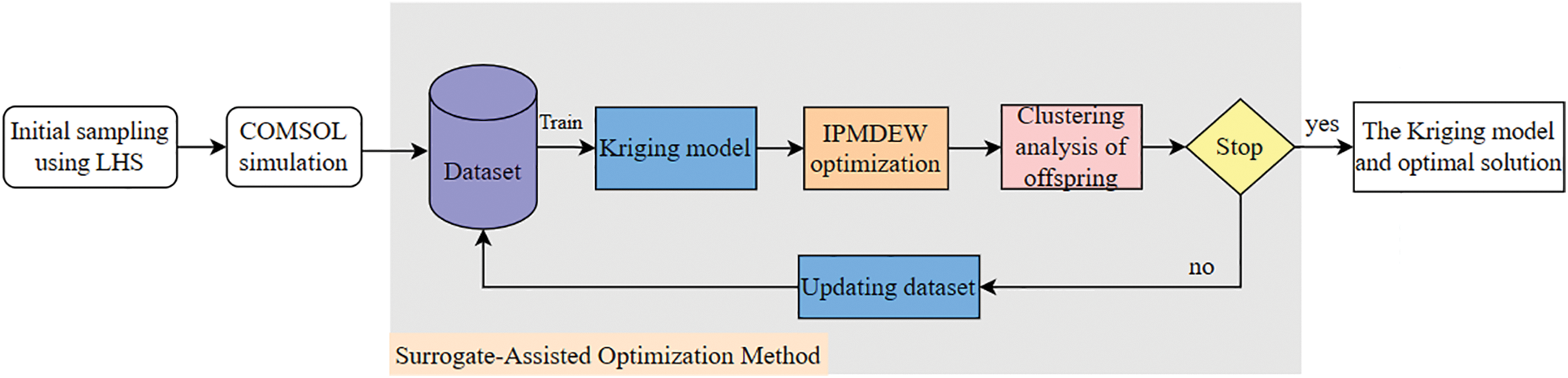
Figure 1: Framework of the Kriging surrogate optimization algorithm.

During the initialization phase, a high-information-density initial sample set is constructed via design of experiments, combining Latin Hypercube Sampling [16] (LHS) with historical datasets. Throughout the iterative optimization process, the Kriging model approximates the objective response values in real time to reduce computational overhead. To overcome the limitations of traditional passive surrogate modeling, an active learning mechanism is proposed: in each iteration, k-means clustering is applied to the offspring population generated by differential evolution. This method screens individuals based on diversity, selecting the most spatially representative candidate solutions for Finite Element validation. This strategy ensures that newly added sample points effectively probe undersampled design subspaces and mitigates the local overfitting of the surrogate model that can result from sample clustering.

2.4 The IPMDEW Algorithm

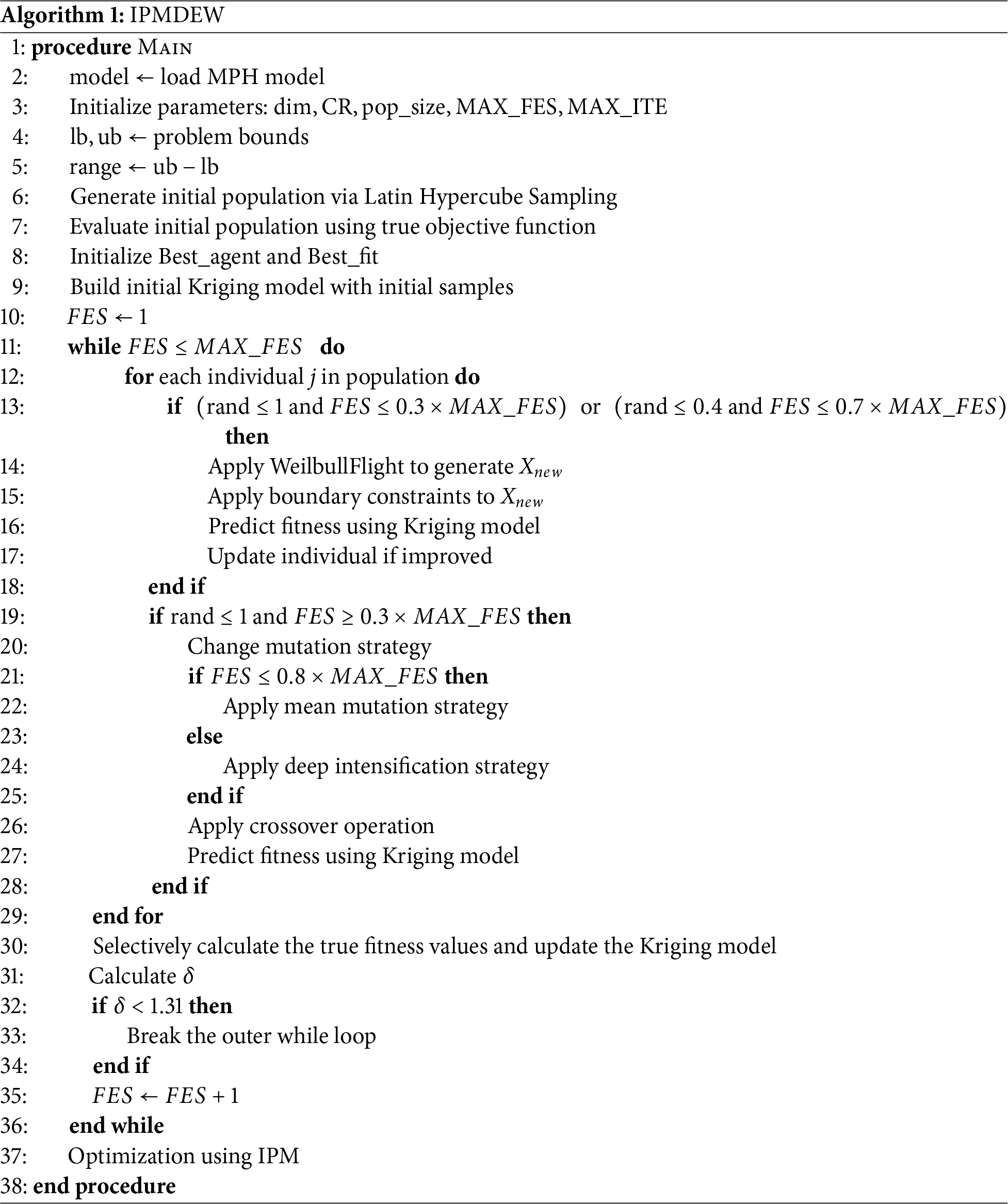
To optimize high-dimensional Kriging models, this paper proposes an integrated algorithm that combines the IPMDEW method (Algorithm 1). The algorithm employs the Weibull distribution-based Weighted Differential Evolution (MDEW) for global exploration. When the population converges, it switches to the Interior Point Method (IPM) for local refinement within the neighborhood of the best solution found. The detailed procedure is illustrated in Fig. 2.

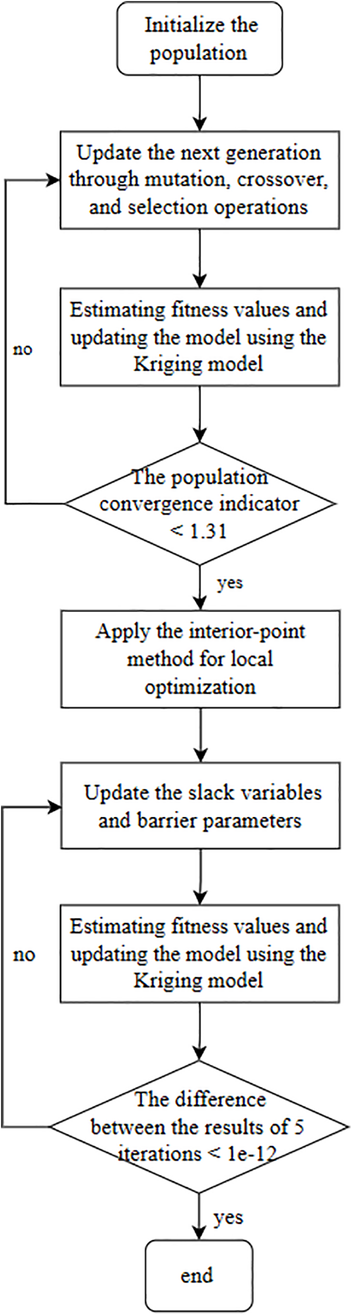
Figure 2: Flowchart of the IPMDEW algorithm.

Step (1) Initialize the population. First, the MDEW algorithm initializes a population randomly, where each individual represents a potential solution xi=[xi,1,xi,2,…,xi,D] (i=1,2,…,NP). To obtain good solutions, the MDEW algorithm emphasizes maintaining diversity in the initial population, which is formed according to the following rule:

xi,j=Lj+rand∗(Uj−Lj)(12)

where Uj, Lj represent the upper and lower bounds, D and NP represent the dimension and population size, rand denotes a random number between 0 and 1.

Step (2) Generate the offspring. Updating the population involves the following procedures.

(1) Introduce three mutation strategies [17], and generate the mutation vector vi following rule:

vi={xi+step                                        g≤0.3∗Gxc1+F(xc1−xi)+F(xc2−xi)     0.3∗G≤g≤0.6∗Gxbest+F(xc1−xi)+F(xc2−xi)   0.6∗G<g<G(13)

where g and G represent the current and maximum iteration, respectively, xbest denotes the current best solution. Step is generated based on the Weibull distribution and the Euclidean distance of the current best solution xbest. Parameter F represents scaling factor. The value of F, xc1, xc2 are computed using the following equations:

F=α+β∗wblrnd(0.5,1,1)(14)

xc1=xr1+xr22(15)

xc2=xr1+xbest2(16)

where α=0.15, β=0.25, xr1 and xr2 are solutions randomly selected from the initial population, and wblrnd denotes a random number generated from a Weibull distribution.

(2) Generate the new crossover vectors as following rule:

ui,G={vi,G    if rand≤CR or j=njxi,G               else(17)

where ui,G represents the new trial vector, nj denotes a random number where nj∈[1,D], and CR indicates the crossover rate within the range of [0, 1].

(3) Push the trial vector to the next generation if it has better fitness.

xi,G+1={ui,G     if f(ui,G)≤f(xi,G)xi,G             else(18)

where f(ui,G) and f(xi,G) are the fitness values of the trial vector and target vector, respectively.

Step (3) Updating the Kriging Model. Offspring are selected using k-means clustering. The selected individuals are then validated through FEA to update both the dataset and the Kriging model.

Step (4) Evaluate the population convergence threshold. To enhance the global search capability of MDEW, a population convergence threshold is defined. the population’s standard deviation in each dimension is calculated as follows:

σk=1NP∑i=1NP(xi,k−μk)2(19)

μk=1NP∑i=1NPxi,k(20)

where xi,k denotes the value of the ith dimension for the kth individual, denotes the mean value of the kth dimension.

The population convergence threshold δ is defined as the mean standard deviation across all dimensions:

δ=1d∑kdσk(21)

Through multiple convergence experiments, the convergence threshold δ in this study is set to 1.31. If δ<1.31, it indicates a high degree of population aggregation. Continuing the optimization using the MDEW algorithm at this stage would be inefficient. The Interior-Point Method (IPM), with its deterministic mathematical programming approach, enables refined local exploitation, effectively compensating for a common limitation of population-based algorithms in having limited exploitation capability and a tendency to stagnate during the final stages of the search. Otherwise, the process returns to repeat Steps 2–4.

Step (5) Construct the approximation function. The approximation function is constructed using the logarithmic potential function and the Lagrange multiplier as follows:

{minx,s⁡fμ(x,s)=minx,s⁡f(x)−μ∑iIn(si)s≥0 ,μ>0, h(x)=0,g(x)+s=0(22)

The added logarithmic term acts as a barrier function, μ and S represent the barrier parameter and slack variable.

Step (6) Update the slack variable and barrier parameter. Each iteration applies either a direct step or a conjugate gradient step, based on an evaluation function defined as:

fμ(x,s)+v||h(x),g(x)+s||(23)

(1) The direct step (Δx,Δs) is defined as:

[H0JhTJgT0Λ0SJh000JgI00][ΔxΔsΔyΔλ]=−[∇f+JhTy+J{g}TλSλhg+s](24)

where Jg and Jh denote the Jacobian matrix of the constraint function g and h, S=diag(s), λ represents the Lagrangian multiplier vector associated with the constraint g, e denotes unit vector, and H=∇2f(x)+∑iλi∇2gi(x).

(2) The conjugate gradient step obtains the Lagrangian multipliers by solving the following equation:

∇xL=∇xf(x)+∑iλi∇gi(x)+∑jλj∇hj(x)=0(25)

When satisfying g(x)+JgΔx+Δs=0,h(x)+JhΔx=0, (Δx,Δs) can be approximately solved using the following equation:

minΔx,Δs⁡∇fTΔx+12ΔxT∇xx2LΔx+μeTS−1Δs+12ΔsTS−1ΛΔs(26)

Due to the black-box nature of the distributed active noise optimal control model, the finite difference method was employed to compute all first- and second-order derivatives. The validity of this method is supported by Refs. [18,19].

The parameter μ is reduced by a certain value if the solution of the approximating function from the previous iteration is meets a predefined accuracy threshold, where the accuracy is defined by:

max(||∇f(x)+JgTλ||,||Sλ−μe||,||h||,||g(x)+s||)(27)

The barrier parameter is updated using the predictor-corrector step [20]. In the predictor step, a linearized step size is employed, and with μ=0, Eq. (24) can be updated as:

[H0JhTJgT0Λ0SJh000JgI00][ΔxΔsΔyΔλ]=−[∇f+JhTy+J{g}TλSλhg+s](28)

Define and as the maximum step sizes that satisfy the constraints.

αs=max(α∈(0,1]:s+αΔs≥0)αλ=max(α∈(0,1]:s+αΔλ≥0)(29)

To evaluate the performance of the prediction-corrector step in updating the barrier parameter, a complementary parameter μp is introduced. It is calculated from the prediction step as follows:

μp=(s+αsΔs)(λ+αλΔλ)m(30)

where m denotes the number of constraints. The first correction step determines the search direction using the following equation:

[H0JhTJgT0Λ0SJh000JgI00][ΔxcorΔscorΔycorΔλ]=−[0ΔSΔλ00](31)

The second correction step, or centering step, is computed by solving the following equation:

[H0JhTJgT0Λ0SJh000JgI00][ΔxcenΔscenΔycenΔλ]=−[∇f+JhTy+J{g}TλSλ−μeσhg+s](32)

where σ=(μp/μ)3

Step (7) Perform iterative operations. If the difference between the results of the last five iterations is less than 10−12, repeat only step 6. Otherwise, continue repeating steps 1–6 until the maximum number of iterations (10) is reached.

3  Experimental Results

The experiments were conducted on a PC running Windows 10 Pro-64 bit, equipped with an Intel(R) Core(TM) i7-6700 CPU @ 3.40 GHz and 16 GB of RAM. The implementation of all pro-posed algorithms was done using MATLAB 9.9 (R2020b).

In the finite element simulation, the computational domain is configured as follows: each wavelength is discretized with no fewer than 8 mesh elements to ensure convergence, and a PML is applied as the absorbing boundary condition. The MUltifrontal Massively Parallel Sparse Direct Solver (MUMPS) is selected for computation, with the relative tolerance set to 0.001. The description related to the Kriging model is as follows: In the Kriging model, the kernel function employs the RBF Gaussian kernel to characterize the correlation structure of spatial data, which effectively captures the similarity between sample points through an exponential form of radial distance. The estimation of hyperparameters is based on a maximum likelihood estimation strategy, where the likelihood function is maximized to optimize model fitting, thereby enhancing prediction accuracy and robustness.

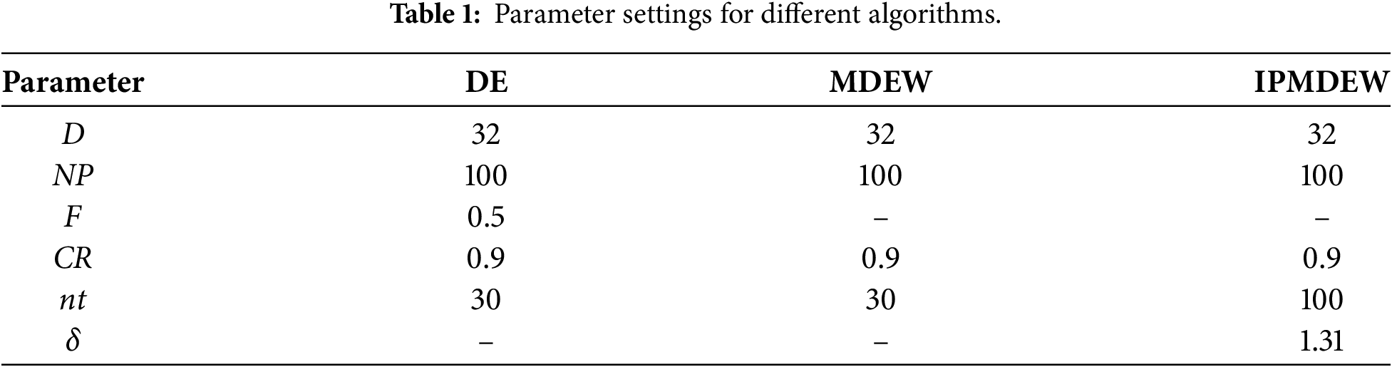
In the experimental design, the IPMDEW algorithm was employed to optimize the Kriging model. To systematically evaluate both the optimization performance of IPMDEW and the prediction accuracy of the Kriging model, multiple comparative schemes were established. For comparative analysis, both the standard DE algorithm and the MDEW algorithm—the latter of which exhibits enhanced global exploration capabilities—were introduced. During the FEA optimization process, key algorithm parameters—including population size (NP), mutation factor (F), crossover probability (CR) and number of iterations (nt)—were systematically varied and compared the variations in noise reduction performance under different parameter combinations. Based on multiple sets of experimental comparisons, the optimal parameter set was ultimately determined, with specific values provided in Table 1. All algorithms used in this study employ this parameter set for subsequent analysis.

To assess the prediction accuracy of the Kriging surrogate model, a test sample set was generated within the parameter space using the LHS method, and the predictions of the Kriging model were compared against FEA.

The DE, MDEW, and IPMDEW algorithms were used to perform twenty independent optimization runs based on the Kriging surrogate model (Figs. 3 and 4). The convergence curves in Figs. 5 and 6, which compare the performance of the three algorithms in both Kriging-based surrogate optimization and Non-surrogate optimization, the IPMDEW algorithm exhibits significant performance advantages in optimizing both the surrogate model and the direct simulation model. These advantages are evident in its faster convergence speed and superior solution quality. Furthermore, Fig. 7 shows that the prediction accuracy of the Kriging model improved consistently throughout the iterative process, eventually stabilizing with minor fluctuations. This validates its reliability as an efficient surrogate model.

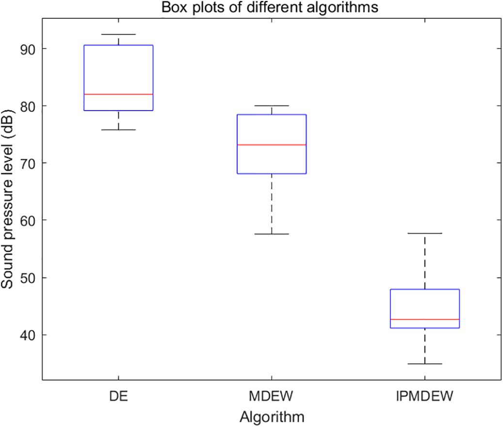
Figure 3: Box plots of multiple runs for different algorithms under surrogate optimization.

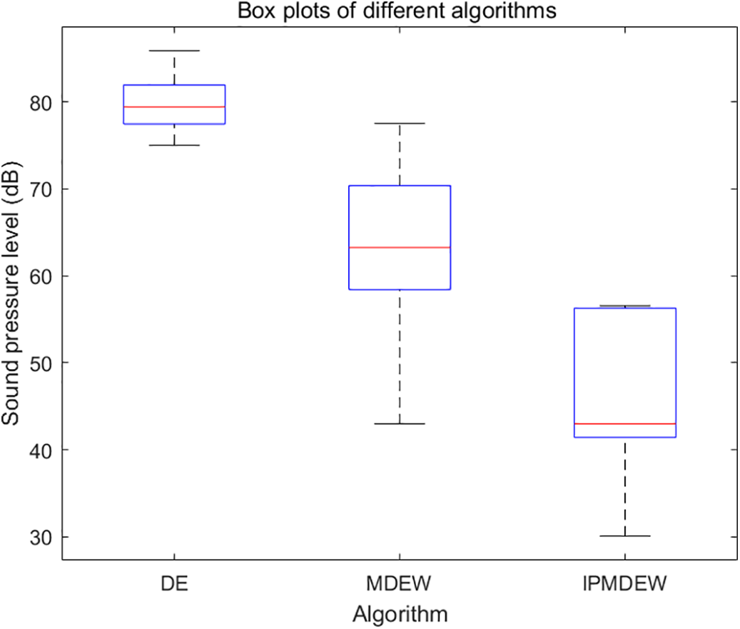
Figure 4: Box plots of multiple runs for different algorithms under Non-surrogate optimization.

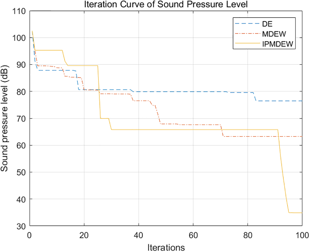
Figure 5: Iteration curves of different algorithms for Kriging surrogate optimization.

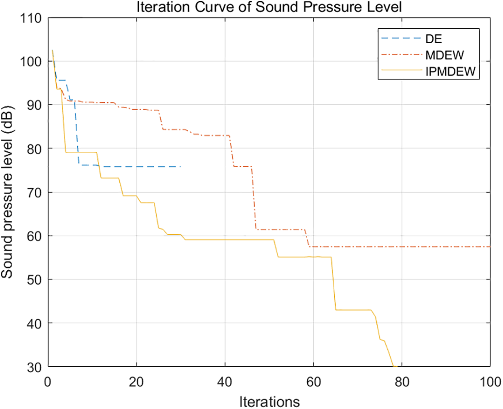
Figure 6: Iteration curves of different algorithms for Non-surrogate optimization.

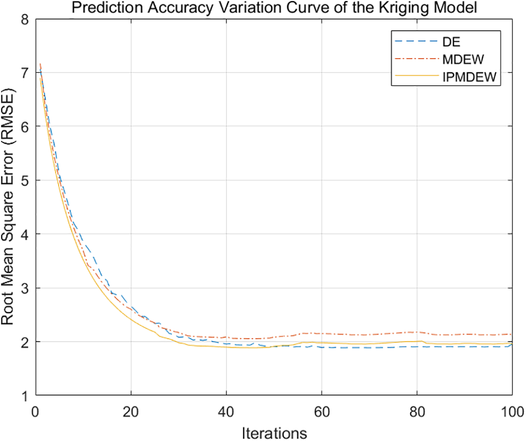
Figure 7: Prediction accuracy variation curve of the Kriging model.

A comparison of the results in Tables 2 and 3 reveal the average performance of differences algorithms under Kriging-based surrogate optimization and Non-surrogate optimization, with the optimization outcomes further validated via finite element analysis. The DE algorithm exhibited premature convergence due to its weak global search capability. Although more effective than DE, the MDEW algorithm was limited by the Kriging model’s prediction accuracy during iterations; as a result, its final noise reduction performance did not reach the optimum achieved by direct simulation. Despite these limitations, the Kriging-assisted optimization approach dramatically improved the optimization efficiency of all algorithms evaluated. The IPMDEW algorithm, however, effectively balancing global exploration and local exploitation. It achieved a noise reduction effect closely approximated the optimum while substantially improving computational efficiency, successfully co-optimizing both performance and efficiency.

To evaluate the predictive capability of the Kriging model for optimal solutions, we validated its optimization results through finite element simulation. Fig. 8 shows a comparison of the spatial sound pressure level distributions before and after optimization achieved by the three algorithms. The errors between the Kriging-assisted optimization results and the FEA results were all within 3 dB, confirming the reliability of the surrogate model.

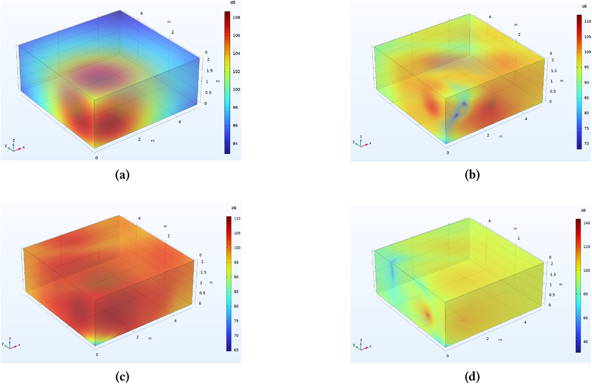
Figure 8: Finite Element validation of Kriging surrogate-assisted optimization under different algorithms. (a) baseline sound pressure level distribution; (b) DE algorithm; (c) MDEW algorithm; (d) IPMDEW algorithm.

4  Conclusion

This paper presents a surrogate-assisted hybrid differential evolution algorithm to address the high-dimensional expensive optimization problem of secondary source deployment in active noise control. By employing a Kriging model as a surrogate for finite element-based sound field simulations, combined with a k-means clustering-based dynamic update mechanism, the computational time for a single sound pressure evaluation was reduced by 85.79%, while model reliability in non-uniform sound fields was maintained. The IPMDEW algorithm integrates the global exploration capability of MDEW with the gradient-based local optimization of the IPM, achieving dynamic switching via a population diversity threshold. Compared to conventional DE and MDEW algorithms, IPMDEW improves noise reduction performance by 67.7% and 48.9%, respectively. The optimized secondary source deployment achieved a noise reduction of 58.32 dB, approaching the accuracy of finite element simulations and validating the algorithm’s effectiveness and precision in complex acoustic environments. This work introduces a surrogate-based hybrid differential evolution approach to acoustic source deployment, providing a practical and efficient solution for optimizing secondary source arrangements in multi-channel spatial active noise control systems. The method has been validated for its reliability in steady sound fields; however, its adaptability to dynamic time-varying acoustic environments, such as those with real-time noise source variations, remains to be investigated. In such scenarios, the existing offline surrogate model update mechanism may struggle to cope with rapid changes, potentially leading to delays in updates and a decline in prediction accuracy.

Acknowledgement: The author would like to express the most sincere gratitude to my supervisor, for his invaluable guidance, continuous support, and patience throughout this study. His profound knowledge and rigorous scientific attitude have been a great asset to my research career.

Funding Statement: The authors received no specific funding for this study.

Author Contributions: Chao Wu: writing—original draft, software, experiment, validation. Weijian Kong: writing—review & editing, methodology, conceptualization. All authors reviewed and approved the final version of the manuscript.

Availability of Data and Materials: Data used to support the findings of this study are included in the article.

Ethics Approval: Not applicable.

Conflicts of Interest: The authors declare no conflicts of interest.

References

1. Brancatia A, Aliabadi MH, Mallardo V. ABEM sensitivity formulation for three-dimensional active noise control. Int J Numer Methods Eng. 2012;90(9):1183–206. doi:10.1002/nme.3369. [Google Scholar] [CrossRef]

2. Sahu N, Wu L, Babu P, Bhavani Shankar MR, Ottersten B. Optimal sensor placement for source localization: a unified ADMM approach. IEEE Trans Veh Technol. 2022;71(4):4359–72. doi:10.1109/TVT.2022.3146603. [Google Scholar] [CrossRef]

3. Liu HQ, Ren ZG, He CL, Du W. A surrogate-assisted differential evolution algorithm with a dual-space-driven selection strategy for expensive optimization problems. Complex Intell Syst. 2025;11(5):230. doi:10.1007/s40747-025-01812-0. [Google Scholar] [CrossRef]

4. Guo XQ, Wei FF, Zhang J, Chen WN. A classifier-ensemble-based surrogate-assisted evolutionary algorithm for distributed data-driven optimization. IEEE Trans Evol Comput. 2025;29(3):711–25. doi:10.1109/TEVC.2024.3361000. [Google Scholar] [CrossRef]

5. Zhou RF, Ren CL, Meng ZY, Zhu HB. Surrogate-assisted differential evolution with search space tightening for high-dimensional expensive optimization problems. IEEE Trans Syst Man Cybern Syst. 2025;55(10):7356–68. doi:10.1109/TSMC.2025.3582897. [Google Scholar] [CrossRef]

6. Liu G, Su X, Zhou R, Liu N, Zhang L, Tian Y. A fast generalized surrogate -assisted evolutionary algorithm for solving expensive constrained optimization problems. J Supercomput. 2025;81(11):1185. doi:10.1007/s11227-025-07660-6. [Google Scholar] [CrossRef]

7. Rahi KH, Singh HK, Ray T. Partial evaluation strategies for expensive evolutionary constrained optimization. IEEE Trans Evol Comput. 2021;25(6):1103–17. [Google Scholar]

8. Zhang J, Li M, Yue X, Wang X, Shi M. A hierarchical surrogate assisted optimization algorithm using teaching-learning-based optimization and differential evolution for high-dimensional expensive problems. Appl Soft Comput. 2024;152:111212. doi:10.1016/j.asoc.2023.111212. [Google Scholar] [CrossRef]

9. Pan JS, Liu N, Chu SC, Lai T. An efficient surrogate-assisted hybrid optimization algorithm for expensive optimization problems. Inf Sci. 2021;561(2):304–25. doi:10.1016/j.ins.2020.11.056. [Google Scholar] [CrossRef]

10. Jin YC. Surrogate-assisted evolutionary computation: recent advances and future challenges. Swarm Evol Comput. 2011;1(2):61–70. doi:10.1016/j.swevo.2011.05.001. [Google Scholar] [CrossRef]

11. Storn R, Price K. Differential evolution: a simple and efficient heuristic for global optimization over continuous spaces. J Glob Optim. 1997;11(4):341–59. doi:10.1023/A:1008202821328. [Google Scholar] [CrossRef]

12. Farda I, Thammano A, Morris J. Differential evolution with self-adaptive mutation and population improvement strategy for optimization problems. IEEE Access. 2024;12:131809–29. doi:10.1109/ACCESS.2024.3460385. [Google Scholar] [CrossRef]

13. Liu X, Sun JY, Zhang QF, Wang Z, Xu Z. Learning to learn evolutionary algorithm: a learnable differential evolution. IEEE Trans Emerg Top Comput Intell. 2023;7(6):1605–20. doi:10.1109/TETCI.2023.3251441. [Google Scholar] [CrossRef]

14. Chew WC, Liu QH. Using perfectly matched layers for elastodynamics. In: Proceedings of the IEEE Antennas and Propagation Society International Symposium, 1996 Digest; 1996 Jul 21–26; Baltimore, MD, USA. p. 366–9. doi:10.1109/APS.1996.549614. [Google Scholar] [CrossRef]

15. Zhan DW, Cheng YS, Liu J. Expected improvement matrix-based infill criteria for expensive multiobjective optimization. IEEE Trans Evol Comput. 2017;21(6):956–75. doi:10.1109/TEVC.2017.2697503. [Google Scholar] [CrossRef]

16. Ioardanis I, Koukouvino C, Silou I. Classification accuracy improvement using conditioned latin hypercube sampling in supervised machine learning. In: Proceedings of the 2022 12th International Conference on Dependable Systems, Services and Technologies (DESSERT); 2022 Dec 9–11; Athens, Greece. p. 1–5. doi:10.1109/DESSERT58054.2022.10018677. [Google Scholar] [CrossRef]

17. Layeb A. Differential evolution algorithms with novel mutations, adaptive parameters, and Weibull flight operator. Soft Comput. 2024;28:7039–91. doi:10.1007/s00500-023-09561-3. [Google Scholar] [CrossRef]

18. Grapiglia GN, Gonçalves MLN, Silva GN. A cubic regularization of Newton’s method with finite difference Hessian approximations. Numer Algorithms. 2022;99(2):607–30. doi:10.1007/s11075-021-01200-y. [Google Scholar] [CrossRef]

19. Andrei N. Diagonal approximation of the hessian by finite differences for unconstrained optimization. J Optim Theory Appl. 2020;185(3):859–79. doi:10.1007/s10957-020-01676-z. [Google Scholar] [CrossRef]

20. Nocedal J, Wright SJ. Interior-point methods for nonlinear programming. In: Numerical optimization. Springer series in operations research and financial engineering. New York, NY, USA: Springer; 2006. p. 563–97. doi:10.1007/978-0-387-40065-5_19. [Google Scholar] [CrossRef]