Cascading Class Activation Mapping: A Counterfactual Reasoning-Based Explainable Method for Comprehensive Feature Discovery

1  Introduction

Recent advances in deep learning–based image classification models have led to significant performance improvements, driving their widespread adoption in various real-world applications such as medical image diagnosis [1,2], biological pattern recognition [3]. Despite these achievements, the inherent black-box nature of deep learning models—namely, the difficulty in understanding the rationale behind their classification decisions—remains an unresolved challenge [4]. This limitation in interpretability has long been recognized, motivating active research in the field of explainable artificial intelligence (XAI) [5,6]. In particular, for convolutional neural network (CNN)-based image classification models, the Class Activation Mapping (CAM) approach [7] and its variants such as Grad-CAM [8] and Score-CAM [9] have become widely used XAI techniques for visualizing the regions that contribute most to a model’s predictions.

However, existing CAM-based methods suffer from fundamental limitations. Most CAM variants tend to highlight only a single discriminative visual cue that the model relies on most heavily for its classification decision [7,10]. While this is useful when the highlighted cue corresponds to a semantically meaningful feature, it becomes problematic when the model focuses on spurious visual artifacts. In such cases, the entire XAI interpretation can be distorted or even rendered meaningless [11,12].

A more fundamental issue is that there is no guarantee the cues visualized by existing CAM methods represent all the evidence the model uses for classification. Hidden behind the visualized dominant cue may lie secondary cues that the model actually relies upon but that remain undiscovered. These hidden cues may, in some cases, constitute more meaningful classification evidence than the dominant one, and failing to discover them leaves our understanding of the model’s decision-making process incomplete. Overcoming this limitation requires asking a counterfactual question: “If this dominant cue were absent, what would the model rely on?”

In real-world data environments, various forms of visual artifacts coexist. In medical imaging, artifacts such as medical device marks, ruler annotations, hair, gel, and dark corner artifacts occurring during dermoscopic examination are frequently observed [13–15]. Even differences between imaging devices, such as variations in saturation, brightness, and hue, can act as artifacts [16]. In drone imagery, shadows [17], and in industrial inspection imagery, specular reflections caused by highly reflective surfaces [18], all serve as potential artifacts. Critically, Winkler et al. [19] demonstrated that surgical skin markings in dermoscopic images can mislead CNN classifiers, causing models to associate these markings with melanoma diagnosis rather than learning from actual pathological features—a clear example of how artifacts can distort not only classification but also the interpretability of model decisions.

Pre-removal or filtering of such artifacts is not only time- and cost-intensive but also carries the risk of discarding diagnostically important features, making it impractical in real-world settings. Particularly in the medical domain, modifying existing clinical routines to avoid artifacts such as surgical skin markings would substantially affect the workflow of medical staff and thus is not a feasible solution [19]. Furthermore, artifact removal does not always lead to performance improvements and, in some cases, may even undermine the robustness of deep learning models [14].

This study proposes a fundamentally different approach from artifact removal. From the perspective that artifacts embedded in an image do not necessarily need to be eliminated if they contribute to classification performance, the goal of this work is not to remove artifacts but rather to ensure that XAI does not overly focus on a single artifact.

We observed that CNNs are easily dominated by strong visual features during the classification process, and CAM likewise tends to highlight only such dominant features. To address the resulting bias in XAI interpretations caused by this structural property, we propose an iterative approach in which the initially most salient feature identified by CAM is deliberately masked, and CAM is then reapplied to the masked residual image. Through this process, other important features that were previously overshadowed by the dominant cue can be sequentially revealed.

We refer to this framework as Cascaded Class Activation Mapping (CasCAM). By progressively masking dominant regions and uncovering subsequent cues, CasCAM enables the comprehensive recovery of the diverse visual evidence actually leveraged by the model. This provides a structural solution for interpreting multiple relevant regions, even in the presence of artifacts.

Our proposed method, CasCAM, is not an ad-hoc invention but rather a principled framework grounded in well-established methodologies. It draws inspiration from several foundational ideas—such as feature sampling in Random Forests, iterative masking in RISE (Randomized Input Sampling for Explanation) [20], and the philosophy of multi-scale representation—while adapting them to the context of explainable AI. In this sense, CasCAM builds upon established principles and extends them to provide a structured solution for visual interpretability.

First, we draw on the philosophy of feature sampling in Random Forests. The concern that “if a model relies excessively on a single dominant feature, other informative cues may never be learned” has long been recognized in machine learning theory. When a strong feature is present, models often fail to learn from other features, as performance can be achieved without them. This was one of the primary motivations for the development of Random Forests, where each tree samples a random subset of features, thereby giving weaker features the opportunity to contribute to the prediction of the target variable. Our problem and solution bear a strong analogy to this situation. When images contain artifacts, models tend to over-rely on these artifacts for classification, causing other important visual features to be overlooked—simply because the classification task can be solved without them. In a manner similar to how Random Forests deliberately suppress dominant features through feature sampling, our approach intentionally removes strong visual cues. This enables other features, previously overshadowed and underutilized, to be more effectively learned.

Second, our approach is inspired by the iterative masking strategy of RISE (Randomized Input Sampling for Explanation) [20]. RISE estimates the importance of each pixel by repeatedly applying random masks to the input image and observing the corresponding changes in the model’s output. While our method also employs masking, it introduces a crucial difference. Instead of generating random masks, we construct meaningful masks based on existing CAM results. Moreover, these masks are not used as the starting point for explanation but rather as elements to be deliberately removed. In other words, we mask out the regions initially highlighted by CAM and then sequentially explore the next most informative cues. Whereas RISE essentially asks, “Is this pixel important?”, our method instead asks, “If this region is removed, where does the model turn its attention next?”

Third, our framework aligns with the philosophy of multi-scale representation, adopting a hierarchical structure of interpretation. Multi-scale approaches aim to decompose complex data into multiple levels for better understanding, and principal component analysis (PCA) represents one of the most common applications of this philosophy [21]. PCA sequentially separates high-dimensional data along axes that explain the largest variance. The first principal component captures the greatest amount of information within the overall covariance structure, while subsequent components explain the remaining variance in directions orthogonal to those already removed. In this way, the dominant information is extracted first, but the remaining components still retain meaningful explanatory value. This multi-scale perspective prevents a single dominant cue from overwhelming the entire explanation and enables information to be separated into progressively interpretable units. Our proposed method follows a similar hierarchical structure: the most dominant region from the initial CAM output is masked out first, and subsequent important features are iteratively explored from the residual information. Through this process, we reveal the order in which the model relies on different pieces of evidence. Each visualization remains partially interpretable, and taken together, they provide a multi-faceted reconstruction of the model’s decision-making criteria.

The main contributions of this study are as follows: First, we provide a practical solution to the failure of XAI in environments where strong visual cues such as artifacts dominate the model’s decision-making. Unlike prior studies that have primarily focused on removing or filtering artifacts [13], our approach leaves artifacts intact while sequentially and hierarchically visualizing diverse visual evidence used by the model, thereby offering trustworthy explanations even in real-world settings. This is particularly valuable in domains such as medicine, where modifying existing clinical routines to avoid artifacts is often infeasible [19]. Second, CasCAM proposes not a specific algorithm but a structural framework, thereby achieving high extensibility. As an architecture-level methodology that is not tied to a particular explanation algorithm, CasCAM can be combined not only with existing CAM-based methods such as Grad-CAM and Score-CAM, but also with future interpretability techniques yet to be developed.

Third, the proposed method is not limited to artifact-containing images but offers general applicability. In typical image classification tasks, models frequently rely excessively on a single dominant visual feature, causing other meaningful cues to be neglected during both learning and interpretation. By iteratively removing the most dominant evidence, CasCAM restores and reveals these overlooked features, enabling a more comprehensive understanding of the model’s decision process.

The remainder of this paper is organized as follows. Section 2 reviews related work, and Section 3 presents the proposed CasCAM methodology in detail. Section 4 reports experimental results across various datasets and scenarios, while Section 6 concludes the paper and discusses directions for future research.

2  Related Works

van der Velden et al. [22] proposed a taxonomy of XAI methods, in which explanation techniques are categorized by format into visual, textual, and example-based explanations, and by methodological characteristics along three dimensions: model-based vs. post-hoc, model-specific vs. model-agnostic, and global vs. local explanations.

CasCAM belongs to the category of visual explanations in terms of explanation format. This is because the method presents the model’s decision rationale not as numerical indicators or textual descriptions, but as visually highlighted regions (e.g., heatmaps or masks) directly on the input image. In other words, since the essence of CasCAM lies in “showing” the cues utilized by the model, it naturally falls under the domain of visual explanations.

From a methodological perspective, CasCAM can be characterized as a post-hoc, model-specific, and local explanation technique. Its post-hoc nature stems from the fact that it analyzes already trained models without requiring structural modifications. The model-specific aspect arises from its direct use of feature maps and activation information generated in the convolutional layers of CNNs. Finally, its local nature is evident in that it visualizes the decision rationale at the level of individual input images rather than providing generalized insights across the entire dataset.

This section focuses on reviewing visual explanation techniques, as CasCAM builds upon and extends the line of saliency mapping approaches—that is, methods that visualize the regions a model deems important during image classification in the form of heatmaps or masks.

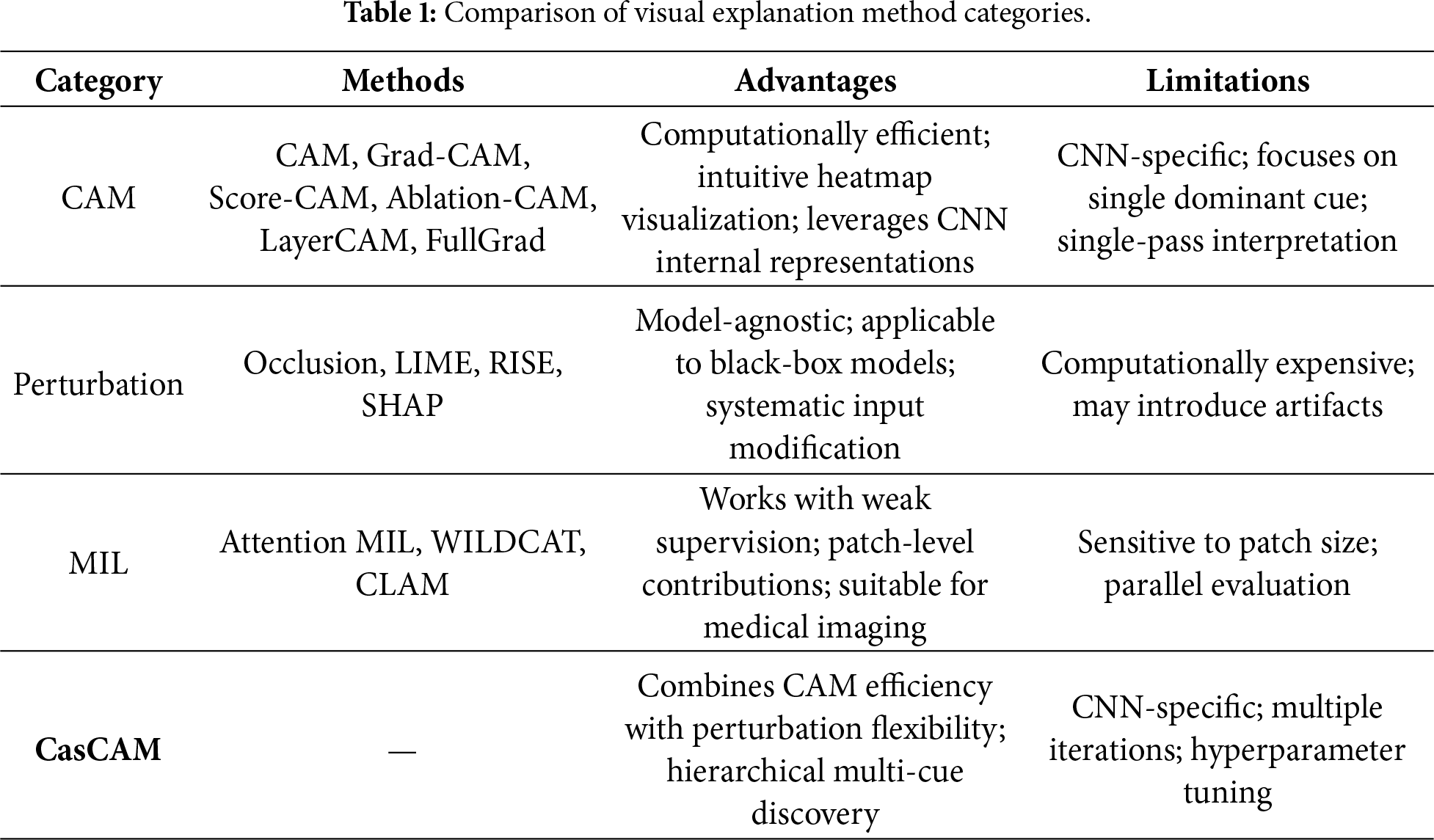
Visual explanation techniques can be broadly categorized into three groups based on their underlying principles. First, CAM and its variants directly visualize the regions a CNN attends to by combining internal feature maps with class-specific information. Methods such as Grad-CAM and Score-CAM fall into this category, leveraging CNN representations most closely at the structural level. Second, perturbation-based methods estimate the relative importance of different image regions by artificially modifying the input (e.g., occluding certain areas, applying blurring, or injecting noise) and analyzing the corresponding changes in model output. Representative examples include Occlusion Sensitivity [23], LIME (Local Interpretable Model-agnostic Explanations) [24], and Meaningful Perturbation [25]. Third, multiple instance learning (MIL)-based methods divide an image into multiple patches and learn or estimate how much each patch contributes to the final prediction. This approach offers the advantage of capturing contributions at the patch level in an aggregated manner.

These three approaches each have their own strengths and limitations, yet they share the common feature of expressing the model’s visual attention in the form of heatmaps or masks, which has established them as representative implementations of XAI. In the following sections, we review these three families of methods in turn and discuss how CasCAM both aligns with and differentiates itself from them.

2.1 CAM and Its Extensions

Zhou et al. [7] introduced CAM, which marked a significant turning point in the interpretation of CNNs. Unlike earlier pixel-level backpropagation-based methods [23,26,27], which often produced noisy and less interpretable results, CAM provided an intuitive way to highlight meaningful object regions through activation maps. Specifically, CAM computes spatial importance by combining feature maps extracted from the last convolutional layer with class-specific weights, introducing a structural modification in which fully connected layers are replaced with global average pooling. This approach offered a clearer visualization of the model’s decision rationale, but it also required changes to the network architecture, limiting its applicability to already trained models.

To address this limitation, Selvaraju et al. [8] proposed Gradient-weighted CAM (Grad-CAM). Grad-CAM generates activation maps by weighting the feature maps with the gradients corresponding to the target class, offering the practical advantage that it can be applied directly without requiring any modification to the existing CNN architecture.

The development of CAM-based methods continued steadily after Grad-CAM. Grad-CAM++ [10] was proposed to mitigate the tendency of Grad-CAM to focus on a single dominant activation. By leveraging higher-order gradient information, it enables more precise highlighting of multiple objects or overlapping patterns, thereby addressing the limitations of CAM-based interpretation in complex images containing multiple visual cues. Score-CAM [9], on the other hand, completely removes dependency on gradient information. Instead, it weights each activation map by the output score obtained after masking the input image with that map, which reduces gradient-induced noise and provides more intuitive and stable explanations. Meanwhile, XGrad-CAM [28] refines the mathematical formulation of the relationship between gradients and activations, thereby enhancing both interpretability and generalization performance.

In addition, a variety of CAM variants have been proposed, including Ablation-CAM [29], LayerCAM [30], HiResCAM [31], FullGrad [32], and Eigen-CAM [33]. Ablation-CAM estimates the contribution of each channel by ablating specific channels in the network, thereby reducing the influence of irrelevant activations and enabling more reliable interpretations. LayerCAM leverages positional information from intermediate layers to highlight fine-grained local cues, making it effective for revealing object substructures. HiResCAM employs high-resolution, pixel-level gradient signals to produce more precise visualizations, while FullGrad integrates gradients across the entire network to provide a global interpretation. Eigen-CAM, on the other hand, applies principal component analysis (PCA) to extract dominant components from feature maps, reducing noise and yielding more stable attention visualizations.

2.2 Perturbation- and Multiple Instance Learning-Based Methods

Perturbation-based methods explain model predictions by deliberately altering the input and analyzing the resulting changes in output. The core intuition is that if masking or distorting a specific region leads to a significant shift in the prediction, that region must be critical for the decision. The early work of Occlusion Sensitivity [23] introduced the idea of covering image patches to measure variations in classification scores. Later, RISE [20] proposed a randomized masking strategy that statistically estimates importance, making it applicable even to black-box models. More sophisticated approaches, such as Meaningful Perturbation [25] and Extremal Perturbation [34], introduced blurring and optimized mask generation to reduce artificial artifacts and provide more stable explanations. Meanwhile, the model-agnostic framework LIME (Local Interpretable Model-agnostic Explanations) [24] approximates local model behavior using simple linear surrogates, offering intuitive interpretations but limited by its reliance on the local linearity assumption. Additionally, SHAP (SHapley Additive exPlanations) [35] applies game-theoretic principles to unify explanations, while counterfactual explanations [36] emphasize how outcomes would differ under alternative inputs.

Multiple Instance Learning (MIL)-based methods are well suited to weakly supervised scenarios. In this framework, an image is divided into patches that together form a bag, and only a global label for the entire bag is provided, while the contribution of each patch is learned. Attention-based MIL [37] assigns weights to patches and interprets them as saliency scores, whereas WILDCAT [38] integrates class-specific feature maps to encourage localization. More recently, CLAM (CLustering-constrained Attention Multiple Instance Learning) [39] has improved both data efficiency and interpretability by generating patch-level importance maps during inference. These methods highlight the synergy between weak supervision and visual explanation, although they remain sensitive to patch size and the interpretability of attention.

2.3 Relationship Between CasCAM and Existing Approaches

Existing visual explanation techniques can be broadly categorized into CAM-based, perturbation-based, and multiple instance learning (MIL)-based methods, each with its own strengths and limitations. The proposed CasCAM is closely connected to all three of these approaches, while simultaneously introducing a novel structure that addresses their inherent constraints.

First, CasCAM directly leverages the core mechanism of CAM within its hierarchical decomposition process. At each stage, it employs the CAM principle to identify the dominant cues for a given class, thereby visualizing the model’s localized decision evidence. In this sense, CasCAM can be regarded as a direct extension of the CAM family of methods.

Second, CasCAM is also connected to perturbation-based approaches in that it intentionally masks the dominant cues detected at each stage and reanalyzes the subsequent model outputs. This inherits the central idea of perturbation-based methods—altering the input to observe the model’s response—while structurally applying it in a recursive manner. As a result, CasCAM enables more systematic and hierarchical interpretation.

Third, CasCAM also shares conceptual similarities with Multiple Instance Learning (MIL)-based approaches. Traditional MIL methods divide an image into multiple patches and evaluate the contribution of each patch. Similarly, CasCAM hierarchically decomposes the input to explore diverse local cues. However, unlike MIL, which typically evaluates patch-level contributions in parallel, CasCAM introduces a hierarchical and iterative structure that progressively removes dominant cues and then investigates the remaining ones. This distinction provides new interpretive possibilities beyond conventional MIL frameworks.

In summary, CasCAM integrates the intuitiveness and interpretability of CAM-based methods, the experimental flexibility of perturbation-based approaches, and the localized exploratory nature of MIL-based techniques. By moving beyond single activation map–centered interpretations, it introduces a novel explanatory framework that can reveal, in a multi-layered manner, the diverse cues actually leveraged by the model.

Table 1 summarizes the characteristics, advantages, and limitations of each category.

3  Cascaded Class Activation Mapping

This section describes the overall procedure of the proposed CasCAM. CasCAM gradually reveals not only the dominant cues that the model initially attends to, but also the hidden supporting cues, through iterative training and masking. All implementation code is publicly available on GitHub1, including training, visualization, and analysis modules to reproduce the experiments.

The dataset consists of input–label pairs (X,y). Here, X∈RH×W×C denotes an image of size H×W with C channels, and y∈{1,…,Ccls} is the class label. The entire original dataset is defined as 𝒟0={(Xn,yn)}n=1N, and the dataset used at the i-th iteration is denoted by 𝒟i. The classification model trained with 𝒟i is represented as f(i). The CAM obtained from model f(i) and input X is defined as M(i)=CAM(f(i),X,y). That is, the CAM visualizes the regions of the image X that support its classification into label y. The resulting CAM M(i) is normalized to the range [0,1] via Min–Max normalization, and, if necessary, resolution normalization is applied to produce M~(i). If a thresholding option TH (e.g., ∅, Top-k, EbayesThresh) is given, the APPLYTHRESHOLD operation is applied as post-processing. The result is stored in CAMs[i][n], and the hyperparameter θ>0 controls the masking strength.

The CAM is not only stored but also used to generate the input for the next iteration. The CAM-based weight is computed as W(i)=exp⁡(−θ⋅M~(i)), where the exponential function provides smooth, continuous suppression of high-activation regions. This formulation ensures that regions with higher CAM values receive stronger suppression (approaching 0), while regions with lower CAM values remain relatively preserved (approaching 1), creating a natural gradient of masking intensity.

The weight is then multiplied with X and normalized to obtain a new image Xres(i)=Norm[0,1](X⊙W(i)), where Norm[0,1](⋅) denotes min–max normalization to [0,1]. The normalization after masking is essential to maintain consistent pixel value ranges across iterations. Without normalization, the progressive masking would continuously reduce pixel magnitudes, leading to increasingly dim images that could destabilize model training and prevent meaningful feature detection in subsequent iterations.

This Xres(i) is added to 𝒟i+1 and used for training in the next iteration. Repeating this process K times produces the stepwise CasCAM set {CAMs[i][n]}i=0,n=1K−1,N, which serves as the main output.

Algorithm 1 formally summarizes this procedure, and Fig. 1 provides a visual illustration of the iterative process. As illustrated in Fig. 1, the CasCAM process begins with the original input image and iteratively generates CAMs while progressively masking dominant features. This example uses the EbayesThresh thresholding scheme, which adaptively determines the threshold based on empirical Bayes estimation, providing robust feature selection without requiring manual tuning of the top-k parameter. In the figure, the top row shows the sequence of CAMs (M(1),M(2),…,M(K)) overlaid on the original image, where each successive CAM reveals different regions as previously highlighted areas are suppressed. The bottom row displays the corresponding residual images (Xres(1),Xres(2),Xres(3)), which serve as inputs for subsequent iterations. The green arrows indicate CAM generation steps, orange arrows represent the masking operation controlled by θ, and the gray arrow shows the final aggregation step where all CAMs are combined using exponentially decaying weights controlled by λ.

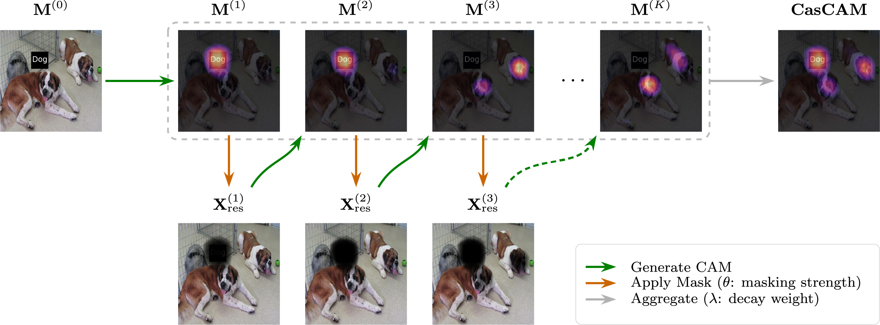
Figure 1: Illustration of the CasCAM generation process using the EbayesThresh thresholding scheme with K=5 iterations and θ=0.3. Starting from the input image M(0), the algorithm iteratively generates CAMs (M(1),M(2),…,M(K)) by progressively masking the dominant features identified in each iteration. The green arrows indicate the CAM generation step using the current model, while the orange arrows represent the masking operation controlled by the threshold parameter θ. The dashed box groups the iteratively generated CAMs, which are then aggregated (gray arrow) using exponentially decaying weights controlled by λ to produce the final CasCAM visualization. The residual images Xres(i) (bottom row) show how the input is progressively modified as dominant features are suppressed, allowing the model to focus on secondary and tertiary features in subsequent iterations.

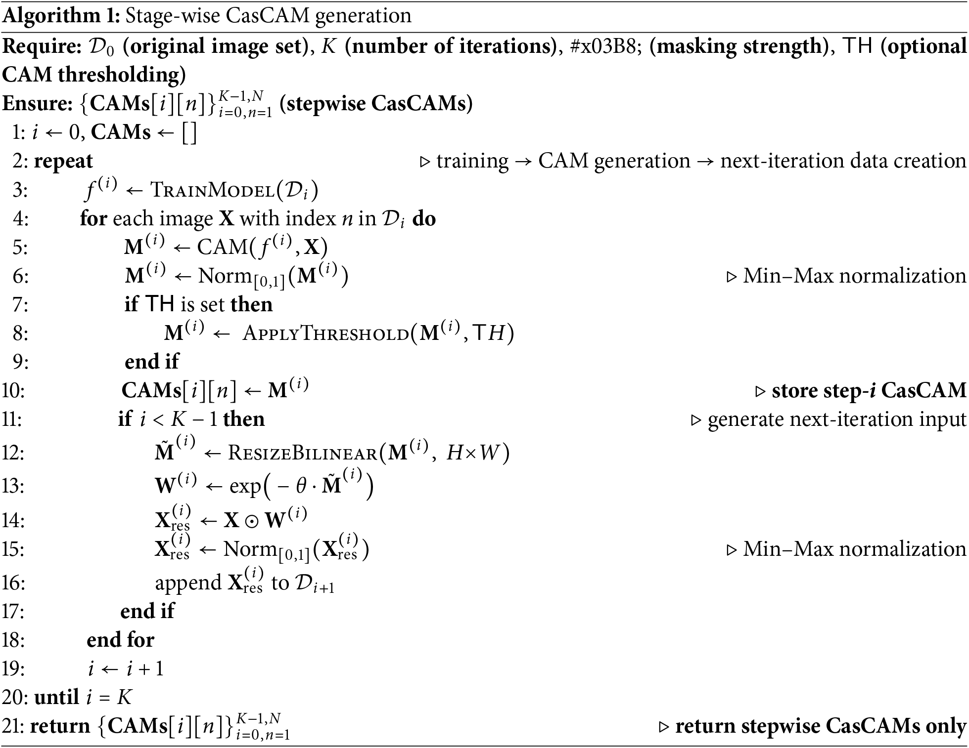
At each iteration, the generated CasCAMs are normalized and stored separately. The final visualization is not derived from a single stage, but instead integrates interpretation maps obtained across multiple stages. To achieve this, each stepwise CasCAM CAMs[i] is combined with an exponential decay weight wi=e−λi∑ℓ=0K−1e−λℓ for i=0,…,K−1, where λ≥0 is the decay rate that determines how strongly the earlier stages are emphasized.

The exponential weighting scheme reflects the natural hierarchy of feature importance: earlier iterations reveal the most dominant features that the model primarily relies on, while later iterations uncover progressively weaker secondary features. By assigning exponentially decreasing weights, we ensure that the final visualization appropriately reflects this hierarchical structure—giving greater prominence to primary features while still incorporating secondary cues. A larger λ places more importance on the dominant features discovered in the initial CasCAMs, whereas λ=0 treats all K stages equally.

The final CasCAM visualization for image n is then given by CasCAMvis[n]=∑i=0K−1wi⋅CAMs[i][n]. Thus, the final result is an integrated interpretation map that captures both the dominant cues revealed in the early iterations and the complementary cues uncovered in the later iterations.

The number of iterations K directly affects both the comprehensiveness and stability of the interpretation. Increasing K allows the method to discover progressively weaker secondary and tertiary features, thereby improving interpretability by revealing a more complete picture of the model’s decision-making process. However, excessive iterations can lead to diminishing returns: as dominant features are repeatedly suppressed, the remaining signal becomes increasingly noisy, and the model may begin attending to spurious patterns rather than meaningful features. This creates a practical trade-off between feature coverage and interpretation reliability.

The optimal value of K depends on both the masking strength θ and image characteristics. Stronger masking (larger θ) suppresses features more aggressively, potentially requiring fewer iterations to reveal secondary features but also increasing the risk of excessive image degradation. Additionally, image characteristics play a crucial role: images with large, prominent objects typically require fewer iterations as dominant features are easily identified and suppressed, while images with small or multiple objects may benefit from more iterations to systematically uncover all relevant features. In our experiments, we use K=5 iterations with θ=0.3 as a reasonable default setting.

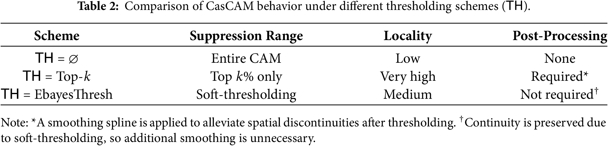
The thresholding scheme TH is a key factor in CasCAM, as it controls the degree of image distortion caused by iterative masking. As the number of iterations increases, the original image may be excessively damaged. Applying thresholding allows only selective suppression of specific CAM regions, producing a more localized weakening effect.

When TH=∅, no thresholding is applied, and the entire normalized CAM is used for masking. In this case, the original image becomes increasingly degraded as iterations progress. On the other hand, TH=Top-k retains only the top k% of CAM values while setting the rest to zero, thus suppressing only the strongest localized features. However, this may cause spatial discontinuities, which are corrected using a smoothing spline. Finally, TH=EbayesThresh employs empirical Bayes soft-thresholding [40], gradually suppressing small values while preserving larger ones. This method exhibits characteristics between TH=∅ and TH=Top-k: it provides localized suppression but in a smoother manner, reducing spatial discontinuities and eliminating the need for additional smoothing.

The differences among the three schemes are summarized in Table 2.

4  Experimental Results

In this section, we validate the performance of the proposed CasCAM by comparing it with existing CAM-based interpretation methods. We selected nine representative CAM-based techniques for comparison: GradCAM [8], GradCAM++ [10], ScoreCAM [9], XGradCAM [28], LayerCAM [30], HiResCAM [31], FullGrad [32], EigenCAM [33], and AblationCAM [29]. All methods were implemented using the pytorch-grad-cam library [41] and compared under identical conditions.

The experimental data was based on the Oxford-IIIT Pet Dataset, modified by inserting “Cat” or “Dog” text labels into each image to create an environment where models could rely on shortcut learning. This setup allows us to evaluate CasCAM’s ability to discover diverse reasoning evidence without relying solely on a single feature. For readers who wish to immediately compare the performance of our method across diverse images (approximately 100 examples), the “Comparison Figures” tab on our project page2 provides interactive visual comparisons with optimally tuned hyperparameters.

4.1 Basic Performance Comparison

In this section, we examine the typical behavior patterns of CasCAM compared to other methods to establish the fundamental performance characteristics. This comparison serves as the foundation for understanding how CasCAM addresses the core limitations of existing interpretation techniques when dealing with confounding visual elements. The results presented here demonstrate the most representative outcomes that illustrate the distinct advantages of our proposed approach over conventional CAM-based methods.

Fig. 2 compares the visualization results of CasCAM with existing CAM techniques on Abyssinian and Egyptian Mau cat images. CasCAM was configured with EbayesThresh thresholding method (TH=EbayesThresh), exponential decay parameter λ=0.2, masking strength θ=0.3, and 5 iterations.

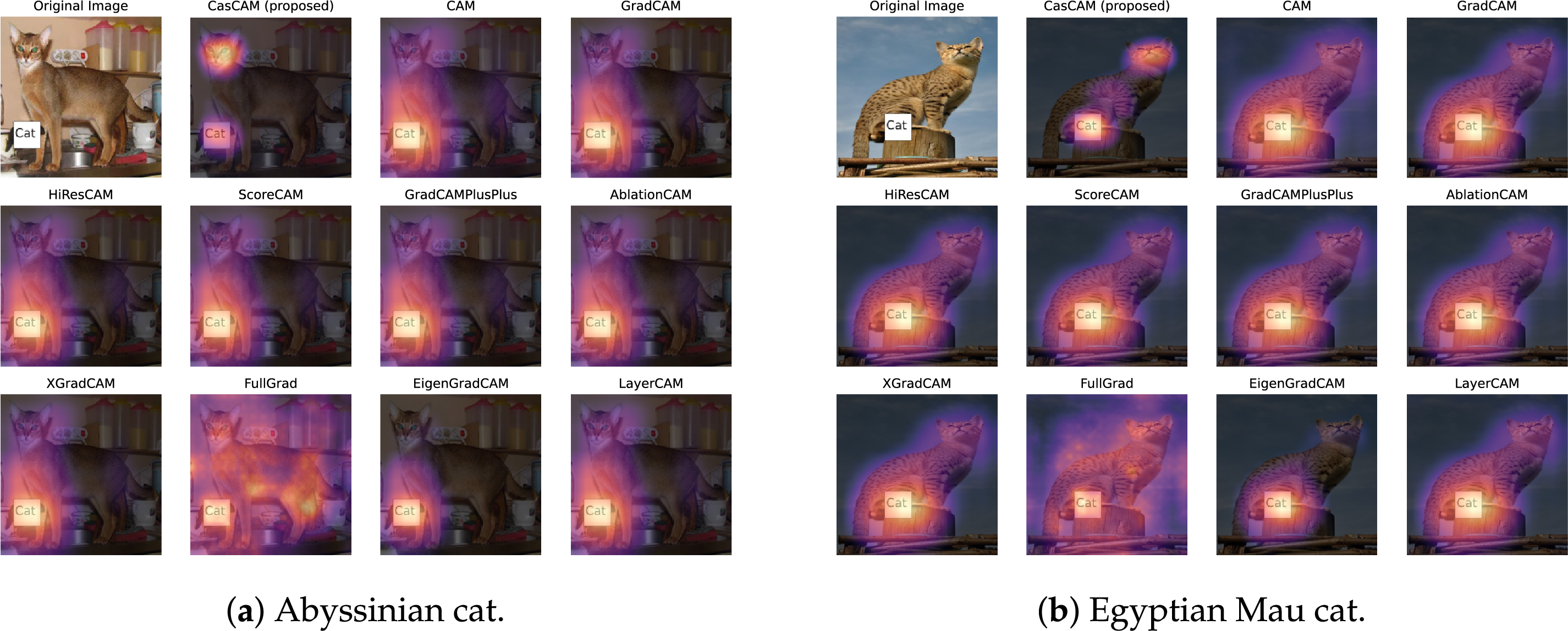
Figure 2: Basic performance comparison between CasCAM and existing CAM techniques. In all heatmaps, warmer colors (red) indicate regions the model considers more important for classification, and cooler colors (blue) represent less important regions. (a) Abyssinian cat image (b) Egyptian Mau cat image.

The comparison results reveal clear distinctions between CasCAM and existing techniques across both cat images. In the Abyssinian cat image (Fig. 2a), most conventional CAM methods—including CAM, GradCAM, HiResCAM, ScoreCAM, GradCAM++, AblationCAM, XGradCAM, LayerCAM, and EigenGradCAM—focus predominantly on the “Cat” text label at the bottom of the image. This demonstrates the shortcut learning phenomenon where the model relies on textual information (confounding elements) rather than the actual visual features of the cat object for classification. FullGrad exhibits widespread activation across the entire image, making specific interpretation challenging.

In contrast, CasCAM displays a distinctly different pattern. The cat’s facial region is accurately emphasized while showing significantly reduced dependence on the text label. This occurs through CasCAM’s hierarchical masking process: when the strongest cue (the text label) is suppressed in the first stage, the model must seek alternative reasoning evidence to achieve the same classification result, thereby bringing the cat’s actual visual features to prominence as the primary dependency targets.

The Egyptian Mau cat image (Fig. 2b) demonstrates consistent behavior patterns. Existing CAM techniques uniformly concentrate on the “Cat” text label while ignoring the genuine feline characteristics. FullGrad again shows diffuse activation throughout the image, limiting interpretability. CasCAM, however, recognizes the text label while simultaneously capturing the cat’s facial features, providing a more comprehensive and reliable interpretation that encompasses multiple reasoning pathways rather than relying on a single dominant cue.

4.2 Localization Performance Analysis

While the previous section examined the overall performance of our proposed method, this section focuses on a specific area where CasCAM demonstrates particular strengths: localization performance. This refers to the ability to localize and leverage small, precise features within an image as reasoning evidence. The proposed method can achieve enhanced localization performance when needed by adjusting parameters—for instance, increasing the number of iterations and localizing the regions to be removed more precisely.

For this analysis, we modified CasCAM’s thresholding method to Top-k (set to 10%) while keeping other parameters unchanged (θ=0.3, λ=0.2, and 5 iterations). The Top-k method selectively processes only the strongest activation regions, which enhances the precision of feature localization compared to the EbayesThresh approach used in the previous section.

To evaluate localization performance, we analyzed results from two different dog breed images. In both experiments, we constructed environments where intentionally inserted text labels act as strong confounding elements, allowing us to observe how each method responds to such interfering factors. The results are presented in Fig. 3.

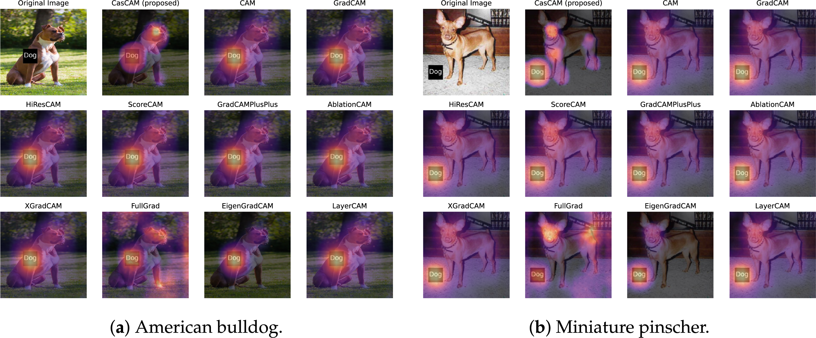
Figure 3: Localization performance comparison using Top-k thresholding method. Heatmap interpretation follows Fig. 2. (a) American bulldog image with central “Dog” text label. (b) Miniature pinscher image with bottom-left “Dog” text label.

The analysis of the American bulldog image in Fig. 3a reveals the localization capabilities of different methods. Despite the presence of a strong confounding element—the central “Dog” label—CasCAM accurately localizes essential features of the dog, including the facial region (particularly the eye area) and legs. This occurs because the Top-k method focuses masking on only the strongest activation regions, allowing relatively weaker signals from actual object features to become clearly prominent in subsequent stages.

Notably, FullGrad also demonstrates interesting behavior, showing widespread activation diffusion while simultaneously focusing on both the confounding element and the dog’s facial and leg features, providing a visualization pattern remarkably similar to CasCAM. This can be attributed to FullGrad’s characteristic of comprehensively reflecting gradients across the entire network to detect diverse features holistically. In contrast, conventional CAM techniques (GradCAM, ScoreCAM, LayerCAM, etc.) all focus exclusively on the confounding element, completely missing essential features.

Similar localization excellence is confirmed in the miniature pinscher image shown in Fig. 3b. Despite the presence of the confounding “Dog” label in the bottom-left, CasCAM evenly localizes various anatomical features of the dog, including the eyes, chest, legs, and hindquarters. This demonstrates that CasCAM’s hierarchical masking process goes beyond simply suppressing a single strong feature—it represents a systematic approach that sequentially uncovers multiple meaningful features that were previously hidden. FullGrad also performs well by properly visualizing the dog’s face and tail regions. However, existing methods continue to show limited performance, being distorted by confounding elements and failing to localize the dog’s essential characteristics.

4.3 Performance in Multi-Artifact Environments

The previous sections demonstrated CasCAM’s effectiveness in handling single confounding elements and its superior localization capabilities. This section examines a more complex and realistic scenario where multiple types of artifacts coexist within the same image. In real-world environments, it is common to encounter not just a single artifact but multiple confounding elements simultaneously.

Fig. 4 examines CasCAM’s performance when multiple confounding elements are present simultaneously. The pug image (Fig. 4a) contains two distinct textual artifacts: Artifact 1 located in the bottom-left center (“Dog” label inserted for experimental purposes) and Artifact 2 in the bottom-right (“Dog” label originally present in the image), along with one essential element—the dog’s facial features. The Samoyed image (Fig. 4b) presents a different configuration with two artifacts of varying nature: Artifact 1 in the top-center (experimentally inserted “Dog” text label) and Artifact 2 in the bottom-center (the Samoyed’s collar, which serves as an indirect rather than direct indicator for dog classification), plus one essential element representing the dog’s facial features.

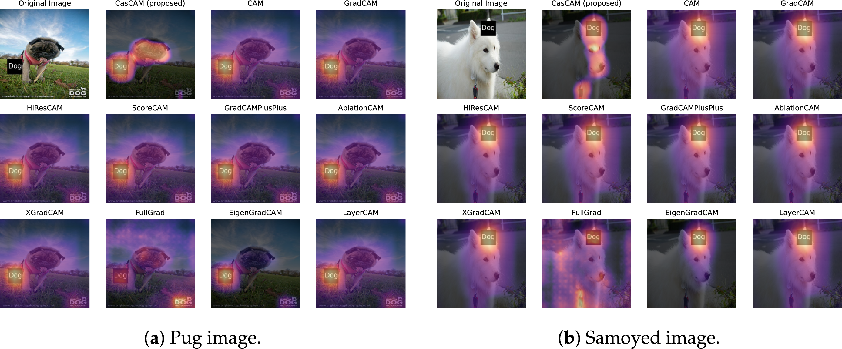
Figure 4: Performance comparison in multi-artifact environments. Heatmap interpretation follows Fig. 2. (a) Pug image with two textual artifacts at bottom-left and bottom-right positions. (b) Samoyed image with top-center text label and bottom-center collar as distinct artifact types.

Most existing CAM methods focus primarily on the experimentally inserted “Dog” label (Artifact 1), largely ignoring the actual dog’s face. Notably, FullGrad concentrates exclusively on the original “Dog” label (Artifact 2) at the bottom-right, completely missing the essential element of the dog’s face. In contrast, CasCAM captures facial features of the dog while simultaneously attending to the textual artifacts. This demonstrates CasCAM’s capability to comprehensively utilize multiple decision grounds rather than relying on a single feature.

In the Samoyed case, FullGrad focuses solely on the collar (Artifact 2), failing to utilize the samoyed’s facial features as decision evidence. Existing CAM methods all concentrate exclusively on the experimentally inserted “Dog” label (Artifact 1) at the top-center. CasCAM visualizes both confounding elements and the essential element of the dog’s face, providing the most comprehensive interpretation among all methods evaluated.

Table 3 summarizes the performance of different CAM methods in detecting various elements within multi-artifact environments. The results reveal distinct patterns in how each method responds to confounding elements. Most existing CAM methods consistently focus on experimentally inserted text labels (Artifact 1) while ignoring essential facial features. FullGrad demonstrates a contrasting behavior by attending exclusively to different artifacts—original text labels in the pug image and the dog collar in the samoyed image—but similarly fails to capture essential elements. Notably, CasCAM is the only method that successfully identifies essential features across both test cases, demonstrating its robustness against multiple types of confounding elements while maintaining comprehensive visual interpretation capabilities.

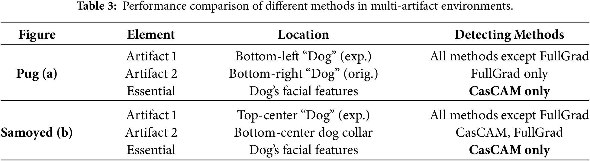
It is worth noting that CasCAM’s failure to visualize Artifact 2 in the pug image is not a good result but rather a disappointing outcome. This is because CasCAM cannot determine whether a particular region is a confounding element or an essential element, but can only evaluate whether that region helps with classification. Therefore, the comprehensive visualization seen in the samoyed image—where all artifacts and essential elements are detected without exception—represents a more desirable result. This performance can be improved through fine-tuning such as lowering the k value and increasing the number of iterations.

4.4 Performance in Multi-Object Environments

The previous sections demonstrated CasCAM’s effectiveness in handling multiple artifacts within single-object scenarios. This section examines a different yet equally challenging scenario where multiple objects coexist within the same image. We conducted experiments using images containing two dogs or two cats to evaluate performance in multi-object environments. This experimental setting presents an interesting contrast to the previous configuration. While the earlier experiments involved two artifacts and one essential element, the current setup features one artifact and two essential elements (though from an AI perspective, these constitute three distinct features requiring attention).

Fig. 5 examines CasCAM’s performance in multi-object environments where multiple essential elements compete for attention. The Saint Bernard image (Fig. 5a) contains one central artifact (experimentally inserted “Dog” text label) and two essential elements—the left dog and the right dog, both of similar size and positioned prominently in the frame. The Bengal cat image (Fig. 5b) presents a more challenging configuration with one top-center artifact (“Cat” label) and two essential elements of varying prominence: a clearly visible central large cat and a smaller cat in the bottom-right that represents a relatively easy-to-miss essential feature due to its size.

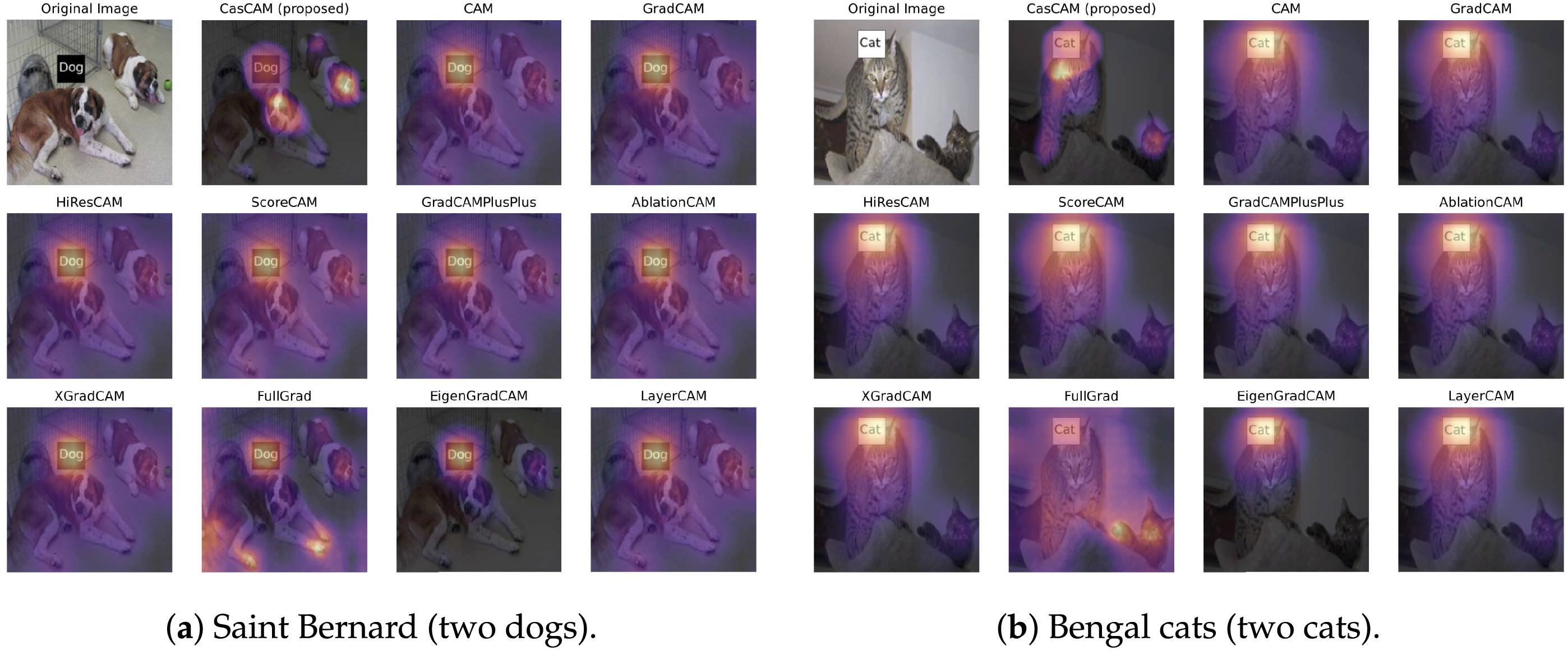
Figure 5: Performance comparison in multi-object environments. Heatmap interpretation follows Fig. 2. (a) Saint Bernard image with one confounding element and two dogs of similar size. (b) Bengal cat image with one text label and two cats of different sizes, where the right-side cat is smaller and more challenging to detect.

FullGrad focuses on peripheral features such as the left dog’s legs and tail rather than its face, and fails to detect the right dog entirely. CasCAM pays attention to the more characteristic facial features of both dogs while recognizing the central artifact. Other existing methods fail to properly identify genuine dog characteristics due to interference from the central artifact.

In the Bengal cat image, the pattern is particularly interesting. CasCAM sequentially visualizes the top-center artifact, the central large cat, and the bottom-right small cat. While the bottom-right small cat is not visualized as prominently as the central large cat, it is still clearly detected. FullGrad shows an overall diffuse pattern that is difficult to interpret, but remarkably provides very clear visualization of the bottom-right small cat’s paws and face. All other methods visualize only the top-center artifact as the basis for classification.

Table 4 summarizes the performance of different CAM methods in multi-object environments where multiple essential elements compete for attention. The results demonstrate distinct patterns in how each method handles artifacts and essential features across different scenarios.

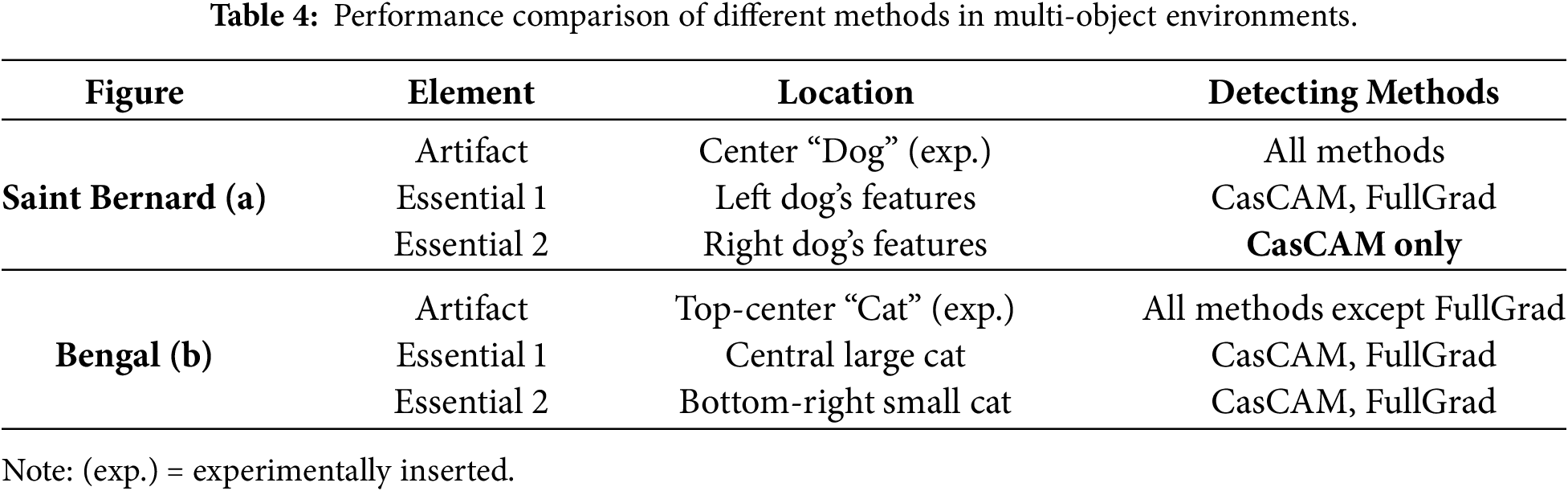
In the Saint Bernard image, all methods successfully detect the central artifact, but their performance on essential features varies significantly. FullGrad detects the left dog’s features (though focusing on peripheral aspects like legs and tail rather than the face) but completely fails to identify the right dog. CasCAM demonstrates superior performance by being the only method that detects both dogs’ essential features while also recognizing the artifact. The Bengal cat image presents a contrasting pattern where FullGrad avoids the top-center artifact entirely but shows remarkable capability in detecting both cats. However, FullGrad’s visualization appears diffuse and difficult to interpret despite clearly highlighting the small cat’s features. Other existing methods focus solely on the artifact, missing essential features entirely. CasCAM again proves its robustness by sequentially visualizing all elements: the artifact, the central large cat, and the bottom-right small cat.

CasCAM’s consistent performance across both scenarios—being the only method to detect the right dog in the Saint Bernard image and successfully handling varying object sizes in the Bengal image—demonstrates its superior capability in multi-object environments where comprehensive feature detection is crucial.

4.5 Quantitative Comparison with Baseline Methods

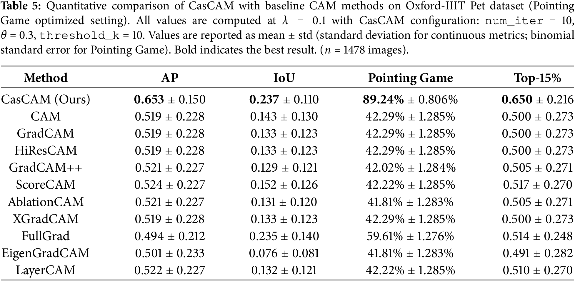
We evaluate CasCAM against ten widely-used CAM-based explanation methods on the Oxford-IIIT Pet dataset. For fair comparison, all methods use the same backbone network (ResNet-50) and target the same convolutional layer for activation extraction. We report four standard localization metrics commonly used in the XAI literature: Average Precision (AP), Intersection over Union (IoU), Pointing Game accuracy, and Top-15% Energy.

Table 5 presents the quantitative comparison results under the Pointing Game optimized setting. CasCAM achieves the best performance across all four evaluation metrics, demonstrating substantial improvements over existing methods. For Average Precision (AP), CasCAM achieves 0.6529, outperforming the second-best method (ScoreCAM, 0.5243) by 24.5%. For Intersection over Union (IoU), which measures the overlap between the predicted saliency region and the ground-truth object mask, CasCAM achieves 0.2366, outperforming all baseline methods; notably, FullGrad achieves competitive IoU (0.2350) but falls significantly behind on other metrics. For Pointing Game accuracy, CasCAM achieves a remarkable 89.24%, substantially outperforming FullGrad (59.61%) and GradCAM (42.29%). For Top-15% Energy, which measures the proportion of saliency energy concentrated within the ground-truth region, CasCAM achieves 0.6499, indicating that nearly 65% of the total saliency energy is focused on the actual object. These consistent improvements demonstrate that CasCAM’s cascade refinement mechanism effectively addresses the fundamental limitations of single-pass CAM methods by progressively suppressing artifact regions while amplifying activations on semantically meaningful object parts.

While Table 5 presents results from the best-performing configuration, we conducted a total of 23 experiments with diverse hyperparameter settings on the Oxford-IIIT Pet dataset to verify the consistency of CasCAM’s performance. Across all configurations, CasCAM consistently outperformed baseline methods. To validate CasCAM’s generalization capability beyond a single dataset, we also evaluated on the MS-COCO dataset with 1,728 images. CasCAM achieves the best AP (0.5417) and Pointing Game accuracy (75.98%), significantly outperforming all baseline methods including FullGrad (+25% relative improvement in AP). Complete results for all 23 configurations and MS-COCO comparisons are available in the “Performance Metrics” tab on our project page3.

Remark (Practical Interpretability Value of Evaluation Metrics): Understanding what these quantitative improvements mean for practical model interpretability is essential for practitioners. Pointing Game accuracy measures whether the model’s peak attention falls within the ground-truth object region; CasCAM’s 89.24% accuracy (vs. GradCAM’s 42.29%) means that practitioners can trust the highlighted region with high confidence—in medical imaging, a clinician can rely on 9 out of 10 visualizations correctly indicating where the model focused its attention. Intersection over Union (IoU) quantifies the spatial overlap between the predicted saliency region and the ground-truth object mask; CasCAM’s IoU of 0.237 (vs. GradCAM’s 0.133) indicates substantially better alignment with actual object boundaries, enabling more precise identification of which specific object parts contributed to the model’s decision. Top-15% Energy measures how concentrated the saliency is within the ground-truth region; CasCAM’s value of 0.650 (vs. GradCAM’s 0.500) indicates that the majority of saliency energy falls within the actual object area, producing more focused visualizations rather than scattered attention patterns that confuse practitioners. Together, these improvements enable more reliable model auditing, facilitate identification of spurious correlations, and support regulatory compliance requirements that demand interpretable decision explanations.

Remark (Statistical Analysis and Effect Sizes): Beyond reporting mean values, we also report standard deviations to support rigorous statistical interpretation. Given the large sample size (n=1478), even trivially small differences would readily achieve statistical significance (e.g., p<0.001), rendering p-values alone insufficient for assessing practical relevance. We therefore emphasize effect size analysis using Cohen’s d=(μ1−μ2)/spooled, where values of 0.2, 0.5, and 0.8 are conventionally interpreted as small, medium, and large effects, respectively.

We first note that FullGrad achieves an IoU nearly identical to that of CasCAM (0.235 vs. 0.237). The corresponding effect size, d=(0.237−0.235)/0.126≈0.02, is negligible, indicating no meaningful practical difference between the two methods in terms of spatial overlap. However, CasCAM exhibits clear advantages on other evaluation metrics. In the Pointing Game, CasCAM (89.24%) substantially outperforms FullGrad (59.61%), yielding an effect size of d≈0.72, which corresponds to a medium-to-large effect. Similarly, for Top-15% Energy, CasCAM (0.650) exceeds FullGrad (0.514) with d≈0.58, representing a medium effect. These results suggest that while both methods achieve comparable overlap with ground-truth regions, CasCAM provides more reliable peak localization and more concentrated saliency distributions—properties that are critical for practical interpretability.

For the remaining baseline methods (GradCAM, HiResCAM, XGradCAM, ScoreCAM, AblationCAM, LayerCAM, EigenGradCAM), CasCAM’s superiority is immediately apparent from Table 5 without requiring formal effect size calculations—these methods achieve substantially lower performance across all four metrics. This consistent and pronounced performance gap confirms that CasCAM’s improvements are practically meaningful.

4.6 Parameter Effects Analysis

CasCAM’s performance is influenced by four primary hyperparameters: the number of iterations (K), masking strength (θ), threshold parameter (k for Top-k), and exponential decay weight (λ). This section provides a systematic analysis of how these parameters affect the model’s behavior and performance.

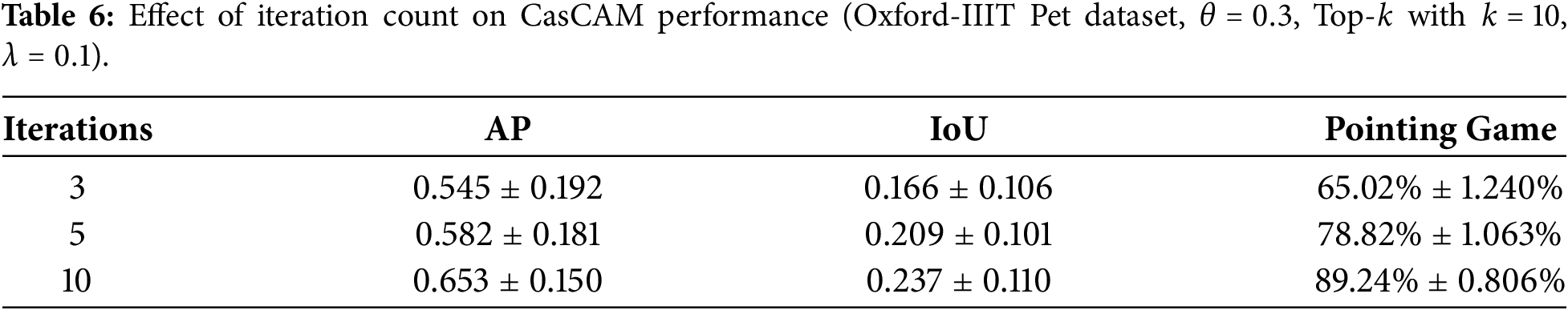
The number of iterations directly impacts interpretation quality. As shown in Table 6, performance consistently improves with more iterations on the Oxford-IIIT Pet dataset. Early iterations (1–3) primarily remove obvious background artifacts, while later iterations (7–10) fine-tune attention to reveal progressively subtler features. The substantial improvement from 3 to 10 iterations (24.2 percentage points in Pointing Game) demonstrates the importance of sufficient iteration depth for comprehensive feature discovery.

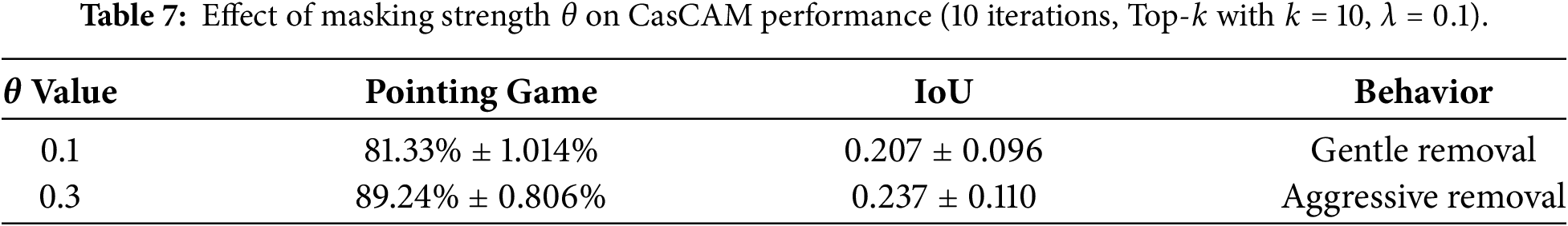
The masking strength θ controls how aggressively the dominant features are suppressed at each iteration. As shown in Table 7, a larger θ value (0.3) achieves 89.24% Pointing Game accuracy compared to 81.33% with θ=0.1. This is because more aggressive suppression leads to faster revelation of secondary features. However, setting θ too high risks excessive image degradation. In our experiments, θ=0.3 provides an optimal balance between feature discovery speed and image preservation.

The choice of thresholding method is critical for CasCAM’s success. Table 8 compares three approaches: Top-k thresholding achieves the best results (89.24% Pointing Game) by focusing suppression on only the most activated regions, allowing the model to maintain sufficient discriminative information for subsequent iterations. EBayesThresh provides an adaptive, data-driven alternative with moderate performance (69.01%). Notably, using no threshold causes excessive image degradation and fails to surpass baseline methods, demonstrating that thresholding is essential—not optional—for CasCAM to function effectively.

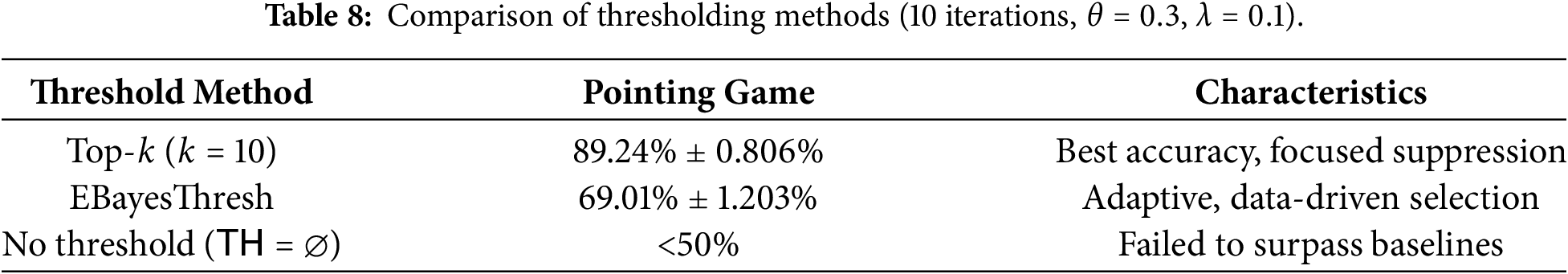
Fig. 6 visualizes how the input images are progressively masked across iterations under different parameter configurations. Each column represents a different combination of threshold method (Top-k with k=10, Top-k with k=20, EBayesThresh) and masking strength (θ=0.1 or θ=0.3). The visualization demonstrates several key observations: (1) higher θ values result in more aggressive masking, causing faster image degradation; (2) Top-k thresholding produces more localized masking compared to EBayesThresh; and (3) smaller k values focus masking on smaller, more concentrated regions.

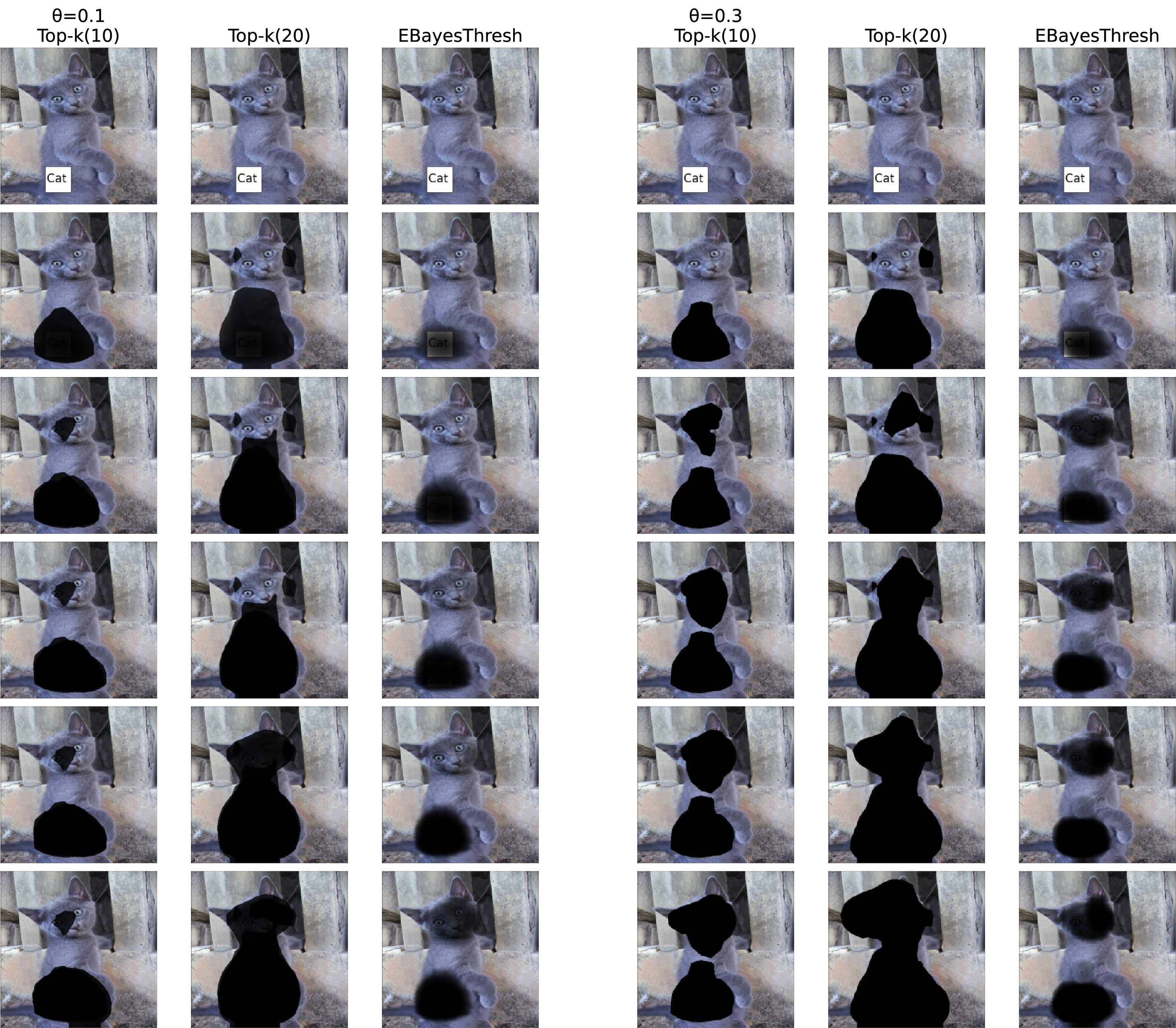
Figure 6: Visualization of progressively masked images across iterations for a Russian Blue cat. Columns represent different threshold methods (Top-k with k=10, Top-k with k=20, EBayesThresh) under two θ values (0.1 and 0.3). Rows show the progression from the original image through selected iterations (1, 3, 5, 7, 9). The no-threshold case (TH=∅) is excluded as it causes excessive degradation.

The exponential decay weight λ controls how the final visualization combines CAMs from different iterations according to wi=e−λi/∑ℓ=0K−1e−λℓ. When λ=0, all iterations are weighted equally, producing broader attention coverage that reveals all discovered features. As λ increases (0.1, 0.3, 0.5), earlier iterations receive progressively more weight, resulting in sharper, more focused attention maps that prioritize dominant features. For applications requiring comprehensive feature coverage (e.g., artifact detection), lower λ values are recommended; for applications prioritizing the most salient features (e.g., object localization), higher λ values may be preferred.

Fig. 7 illustrates this effect. The first two rows show individual CAMs generated at each iteration, where earlier iterations capture dominant features (such as the text artifact) and later iterations reveal secondary features (the dog’s actual body parts). The third row demonstrates how different λ values affect the combined visualization: higher values (λ=0.5) produce sharper maps emphasizing early-iteration features, while lower values (λ=0) create broader coverage by equally weighting all iterations. This flexibility allows practitioners to tune the visualization characteristics based on their specific interpretation requirements.

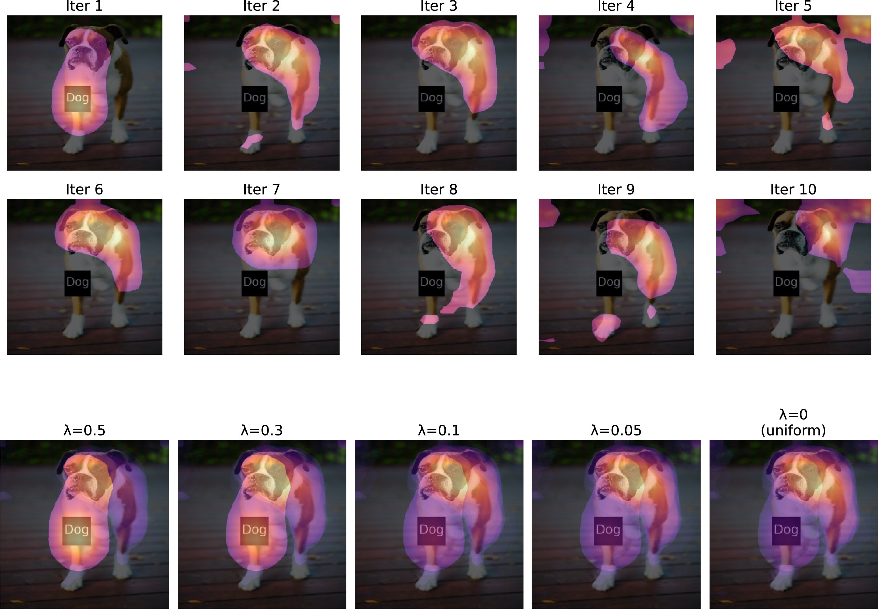
Figure 7: Effect of λ on CasCAM combination for a Boxer dog image (θ=0.3, Top-k with k=20, 10 iterations). Rows 1–2: Individual CAMs at each iteration showing progressive feature discovery from dominant (text artifact) to secondary features (dog’s body). Row 3: Combined CasCAM visualizations with different λ values (0.5, 0.3, 0.1, 0.05, 0), demonstrating the trade-off between focused and comprehensive attention coverage.

4.7 Computational Cost Analysis

CasCAM employs an iterative training-inference loop that differs fundamentally from conventional CAM methods, making direct computational comparison challenging. While traditional methods apply a single forward pass to generate visualizations, CasCAM trains multiple models across iterations, each learning from progressively masked images. This section provides a detailed breakdown of computational costs by process component.

Table 9 shows the training time for different iteration configurations. Notably, training time does not increase linearly with iterations because progressively masked images become harder to classify, triggering early stopping more frequently in later iterations. As shown in Table 10, early stopping rates increase substantially in later iterations due to diminishing discriminative information in progressively masked images, which explains why total training time grows sub-linearly with iteration count.

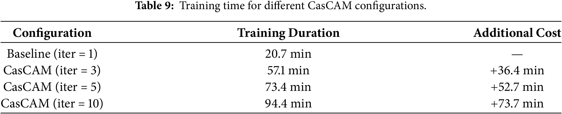
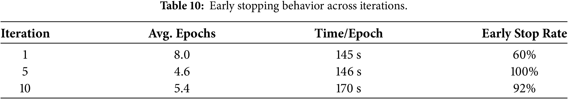
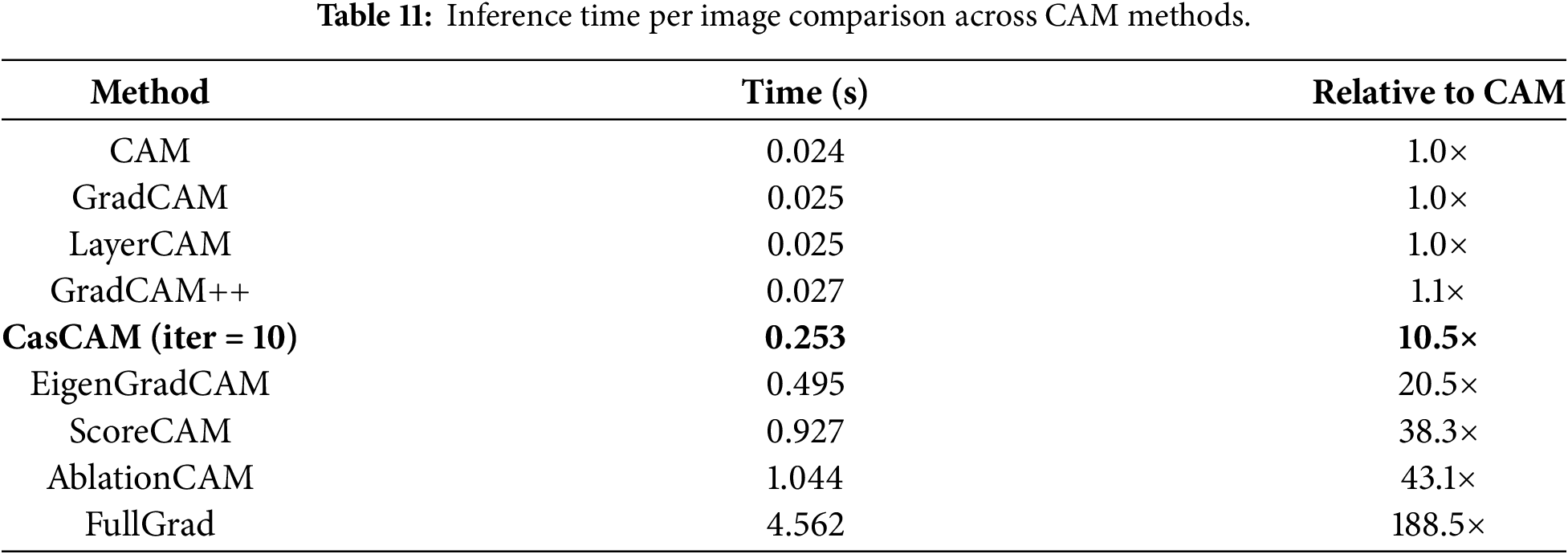
Table 11 presents inference time per image across CAM methods. CasCAM’s inference time can be approximated as tCasCAM≈0.015+0.024×K seconds, where K is the number of iterations.

The total computational cost combines training overhead with inference time scaled by dataset size: Ttotal=Ttrain+N×tinference. Table 12 compares total processing time for different methods across various dataset sizes.

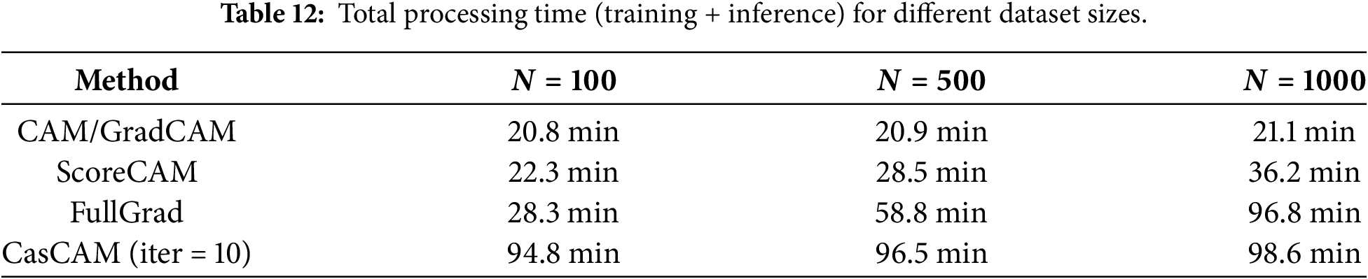
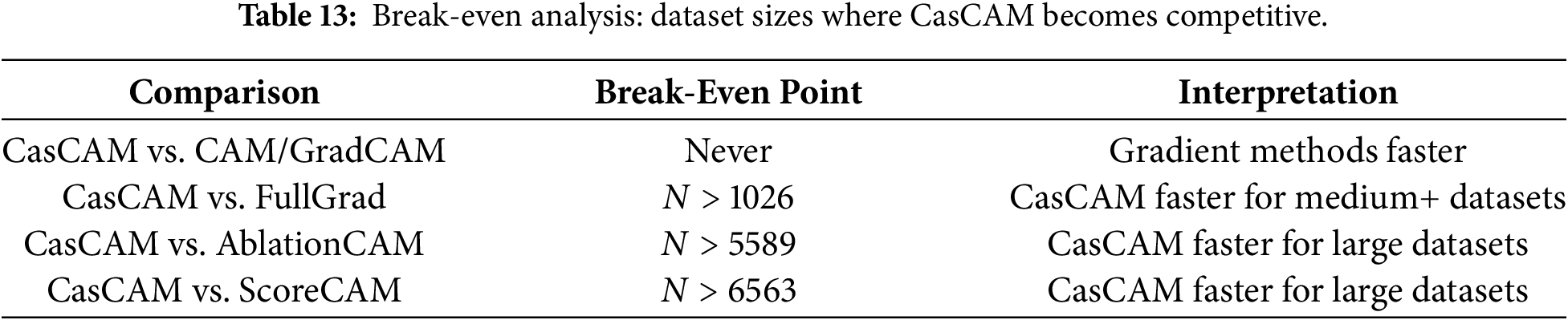
Table 13 presents the break-even analysis, showing the dataset sizes at which CasCAM becomes computationally equivalent to or faster than alternative methods. Gradient-based methods (CAM, GradCAM) always remain faster due to their minimal overhead. However, CasCAM becomes more efficient than FullGrad for datasets exceeding approximately 1000 images, offering better localization accuracy at comparable or lower total computational cost.

In practical deployment scenarios, however, classification models are typically trained once and then deployed for repeated inference on new images. For such inference-only use cases—where a pre-trained model generates CAM visualizations without additional training—only the per-image inference time matters, as training cost is amortized over all subsequent operations. With K=10 iterations, CasCAM requires only 0.253 s per image—approximately 4 images per second—which is 3.7× faster than ScoreCAM (0.927 s), 4.1× faster than AblationCAM (1.044 s), and 18× faster than FullGrad (4.562 s). For applications requiring faster throughput, the number of iterations can be reduced: K=5 yields approximately 7 images per second, while K=3 achieves approximately 11 images per second. This flexibility allows practitioners to balance between comprehensive feature discovery and processing speed.

Based on our analysis, we provide the following practical guidelines: (1) for real-time applications requiring maximum speed, use gradient-based methods (CAM, GradCAM) with approximately 0.025 s per image; (2) for applications prioritizing comprehensive feature discovery with reasonable speed, CasCAM with K=5–10 iterations offers superior localization accuracy while remaining faster than ScoreCAM, AblationCAM, and FullGrad; (3) for small-scale offline analysis (N<1000) where training overhead is a concern, consider FullGrad if accuracy is prioritized; (4) for large-scale analysis (N>1000), CasCAM offers better localization accuracy than FullGrad at comparable or lower total computational cost; and (5) CasCAM with 3–5 iterations provides a practical compromise between training time and performance improvement.

Remark (Memory Usage and Hardware Considerations): All experiments were conducted on a single NVIDIA A100-SXM4-80GB GPU using 512×512 pixel images with batch size 64, consuming approximately 27 GB of peak GPU memory during training. This memory consumption is dominated by the standard ResNet-50 training requirements (model parameters, intermediate activations, and gradients), not by CasCAM-specific overhead.

CasCAM’s additional memory overhead for storing intermediate CAM outputs is minimal. Each CAM is computed at the spatial resolution of the final convolutional layer (7×7 for ResNet-50) and stored at this resolution; upsampling to the original image size occurs only once during final visualization. Thus, storing K=10 iteration CAMs requires only 10×7×7×4=1.96 KB per image in single-precision floating point—negligible compared to model weights (∼100 MB) or a single input image tensor (∼3 MB for 512×512×3 in FP32).

5  Discussion

The multi-cue discovery capability of CasCAM has significant practical implications. In medical imaging, where explainability has become increasingly critical for clinical deployment [42–45], clinicians can verify whether a diagnostic model’s prediction is based on actual pathological features (e.g., lesion characteristics) or on imaging artifacts (e.g., acquisition markers, device-specific patterns), thereby enhancing clinical trust and enabling more informed decision-making.

It is important to note that CasCAM is not a standalone XAI method that exists alongside CAM, Grad-CAM, or Score-CAM at the same conceptual level. Rather, it is a meta-framework—analogous to concepts like ensemble learning or stacking in machine learning—that operates at a higher architectural level. Just as ensemble methods combine multiple base learners rather than competing with them, CasCAM can be applied on top of any existing visualization method through iterative application with counterfactual reasoning. The cascaded framework can be instantiated as Cas-CAM (using CAM as the base method), Cas-GradCAM (using Grad-CAM), Cas-ScoreCAM (using Score-CAM), Cas-FullGrad (using FullGrad), and so on. More generally, the iterative process does not even require using the same method at each iteration—it is possible to use CAM in the first iteration, Grad-CAM in the second, and Score-CAM in the third. This flexibility is a fundamental characteristic of the meta-framework design. Therefore, if a practitioner finds that a particular method (e.g., FullGrad) works well for their specific application, we do not suggest replacing it with CasCAM. Instead, we propose considering the cascaded version (e.g., Cas-FullGrad) to reveal multiple hierarchical features that might be overshadowed in a single iteration. The key advantage is clear: when any single-iteration method fails to capture all relevant features at once, applying it iteratively within the cascaded framework can systematically uncover the full spectrum of visual evidence used by the model.

Despite these advantages, CasCAM involves multiple hyperparameters—including the number of iterations K, the masking strength θ, and the thresholding parameter (e.g., Top-k percentage)—and tuning these appropriately can be challenging. Suboptimal parameter choices may result in CasCAM failing to capture distinctive features clearly, as illustrated in Fig. 8. Fig. 8a shows a multi-object scenario where two cats are present, but CasCAM with suboptimal parameters detects only one object while missing the other. Fig. 8b demonstrates a case where the method becomes overly focused on local features, failing to capture the broader distinctive characteristics of the target object. In such cases, increasing the number of iterations K, or adjusting θ and k to larger values, can help discover more comprehensive features. We encourage practitioners to experiment with different parameter combinations and select the values that best suit their specific application. Nevertheless, some practical guidance can be offered. As a starting point, we recommend K=5 iterations, θ=0.3, and a Top-k threshold of k=20%. From this baseline, users may adjust parameters according to their needs—for instance, reducing the Top-k percentage while increasing the number of iterations to achieve finer-grained feature discovery, or vice versa for faster but coarser exploration.

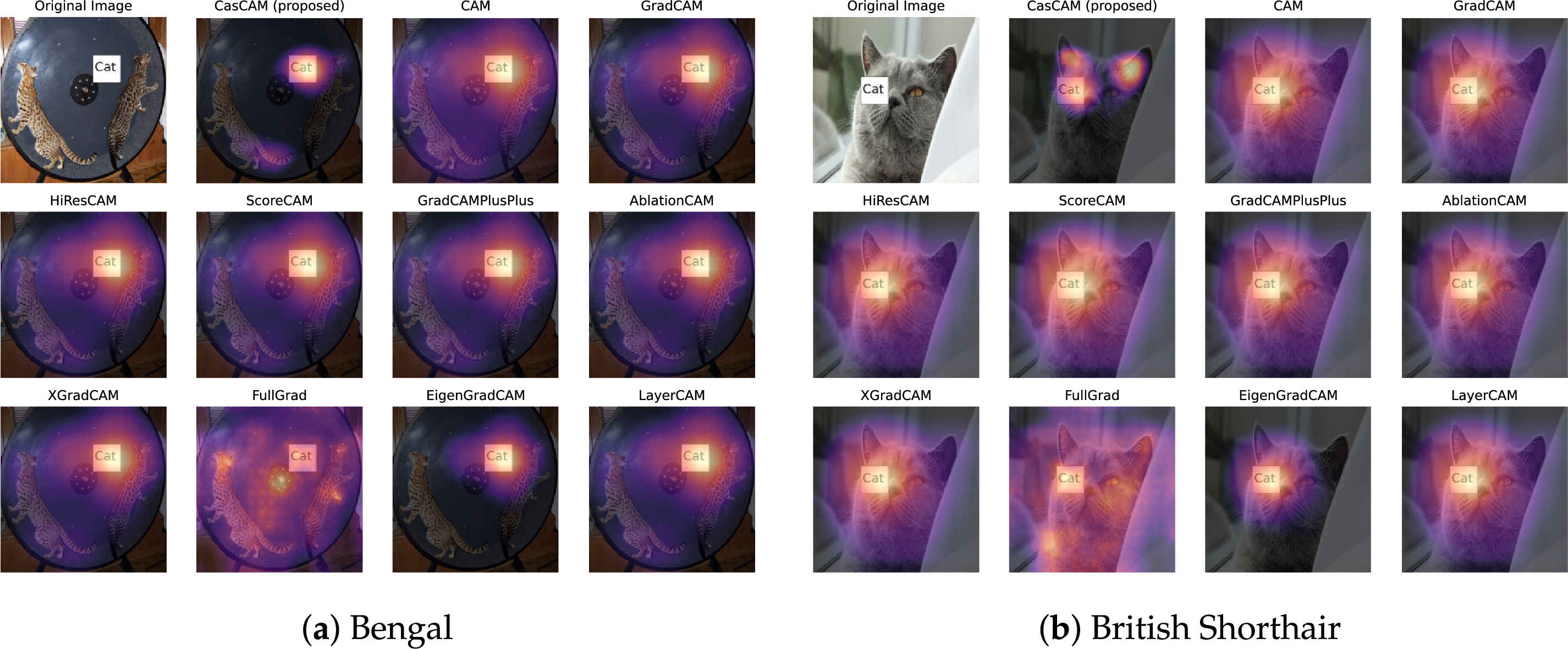
Figure 8: Examples illustrating CasCAM limitations with suboptimal parameters. (a) In a multi-object image containing two cats, only the tail of one cat is barely detected while the other cat is completely missed. (b) The method becomes overly focused on localized features, missing broader object characteristics. These cases suggest that increasing K, θ, or k may help capture more comprehensive features.

However, some limitations should be acknowledged. The masking strength parameter θ controls the spatial extent of feature suppression, which ideally should be adapted to the object scale. When a dataset contains objects of uniform size, an optimal θ can be determined and applied consistently. However, when object sizes vary significantly within a dataset—for example, when some images contain large dominant objects while others contain small localized features—a single fixed θ may not be optimal for all cases. A θ tuned for large objects may overlook small features, while a θ tuned for small objects may require excessive iterations for large objects. Future work could explore adaptive mechanisms that automatically adjust the masking strength based on the detected feature scale, or develop multi-scale approaches that simultaneously operate at different θ values.

6  Conclusion

The proposed CasCAM presents a novel approach that addresses fundamental limitations of existing XAI techniques. Traditional CAM-based interpretation methods have focused on describing the current state of “where the model looked.” However, deep learning models often rely on only one or two strongest visual cues due to shortcut learning, and existing methods visualize only these dominant cues, failing to reveal other meaningful features that models could potentially utilize. CasCAM overcomes these limitations by performing interpretation from a counterfactual reasoning perspective, asking “If this feature were absent, what other evidence would the model use to reach the same conclusion?” By systematically removing the most dominant features and sequentially exploring secondary features that the model would attend to, CasCAM uncovers various decision grounds that are learned within the model but remain hidden beneath stronger features.

Comprehensive experiments confirmed that CasCAM consistently demonstrates superior performance across various artifact environments and complex multi-object scenarios. This research transforms the XAI paradigm from “explanation” to “exploration,” from “current state description” to “potential possibility discovery,” and from “single evidence presentation” to “multi-evidence systematization.” CasCAM functions as a tool that explores the entire spectrum of a model’s potential interpretive capabilities, going beyond simply observing the model’s current state to provide deeper and more reliable understanding of AI model decision-making processes.

Acknowledgement: Not applicable.

Funding Statement: This research was supported by the Basic Science Research Program through the National Research Foundation of Korea (NRF), funded by the Ministry of Education (RS-2023-00249743).

Author Contributions: Seoyeon Choi: Software, Validation, Formal analysis, Investigation, Data curation, Writing—original draft, Visualization. Hayoung Kim: Software, Validation, Formal analysis, Investigation, Data curation, Writing—original draft, Visualization. Guebin Choi: Conceptualization, Methodology, Writing—review & editing, Supervision, Funding acquisition. All authors reviewed and approved the final version of the manuscript.

Availability of Data and Materials: The implementation code and experimental results are publicly available at: Source code: https://github.com/guebin/cascam; Interactive result visualization: https://guebin.github.io/cascam-results/; MS-COCO dataset (with artifacts): https://github.com/guebin/coco-catdog-cascam; Oxford-IIIT Pet dataset (with artifacts): https://github.com/guebin/oxford-pets-cascam.

Ethics Approval: Not appllicable.

Conflicts of Interest: The authors declare no conflicts of interest.

1https://github.com/guebin/cascam

2https://guebin.github.io/cascam-results/

3https://guebin.github.io/cascam-results/

References

1. Litjens G, Kooi T, Bejnordi BE, Setio AAA, Ciompi F, Ghafoorian M, et al. A survey on deep learning in medical image analysis. Med Image Anal. 2017;42(13):60–88. doi:10.1016/j.media.2017.07.005. [Google Scholar] [PubMed] [CrossRef]

2. Esteva A, Kuprel B, Novoa RA, Ko J, Swetter SM, Blau HM, et al. Dermatologist-level classification of skin cancer with deep neural networks. Nature. 2017;542(7639):115–8. doi:10.1038/nature21056. [Google Scholar] [PubMed] [CrossRef]

3. Moen E, Bannon D, Kudo T, Graf W, Covert M, Van Valen D. Deep learning for cellular image analysis. Nature Meth. 2019;16(12):1233–46. doi:10.1038/s41592-019-0403-1. [Google Scholar] [PubMed] [CrossRef]

4. Castelvecchi D. Can we open the black box of AI? Nature News. 2016;538(7623):20. doi:10.1038/538020a. [Google Scholar] [PubMed] [CrossRef]

5. Zhang X, Chan FTS, Mahadevan S. Explainable machine learning in image classification models: an uncertainty quantification perspective. Knowl Based Syst. 2022;243:108418. doi:10.1016/j.knosys.2022.108418. [Google Scholar] [CrossRef]

6. Akhtar NA. A survey of explainable AI in deep visual modeling: methods and metrics. arXiv:2301.13445. 2023. [Google Scholar]

7. Zhou B, Khosla A, Lapedriza A, Oliva A, Torralba A. Learning deep features for discriminative localization. In: Proceedings of the IEEE Conference on Computer Vision and Pattern Recognition. Las Vegas, NV, USA: IEEE; 2016. p. 2921–9. [Google Scholar]

8. Selvaraju RR, Cogswell M, Das A, Vedantam R, Parikh D, Batra D. Grad-CAM: visual explanations from deep networks via gradient-based localization. In: Proceedings of the IEEE International Conference on Computer Vision. Venice, Italy: IEEE; 2017. p. 618–26. [Google Scholar]

9. Wang H, Wang Z, Du M, Yang F, Zhang Z, Ding S, et al. Score-CAM: score-weighted visual explanations for convolutional neural networks. In: Proceedings of the IEEE/CVF Conference on Computer Vision and Pattern Recognition Workshops. Seattle, WA, USA: IEEE; 2020. p. 24–5. [Google Scholar]

10. Chattopadhay A, Sarkar A, Howlader P, Balasubramanian VN. Grad-CAM++: generalized gradient-based visual explanations for deep convolutional networks. In: 2018 IEEE Winter Conference on Applications of Computer Vision (WACV). Lake Tahoe, NV, USA: IEEE; 2018. p. 839–47. [Google Scholar]

11. Adebayo J, Gilmer J, Muelly M, Goodfellow I, Hardt M, Kim B. Sanity checks for saliency maps. Adv Neural Inf Process Syst. 2018;31(5):175–84. doi:10.1007/978-3-031-16564-1_17. [Google Scholar] [CrossRef]

12. Ghorbani A, Abid A, Zou J. Interpretation of neural networks is fragile. In: Proceedings of the AAAIConference on Artificial Intelligence. Vol. 33. Honolulu, HI, USA: AAAI Press; 2019. p. 3681–8 [Google Scholar]

13. Jamil U, Akram MU, Khalid S, Abbas S, Saleem K. Computer based melanocytic and nevus image enhancement and segmentation. Biomed Res Int. 2016;2016(1):2082589. doi:10.1155/2016/2082589. [Google Scholar] [PubMed] [CrossRef]

14. Pewton SW, Cassidy B, Kendrick C, Yap MH. Dermoscopic dark corner artifacts removal: friend or foe? Comput Methods Programs Biomed. 2024;244:107986. doi:10.1016/j.cmpb.2023.107986. [Google Scholar] [CrossRef]

15. Jütte L, Patel H, Roth B. Advancing dermoscopy through a synthetic hair benchmark dataset and deep learning-based hair removal. J Biomed Opt. 2024;29(11):116003. doi:10.1117/1.jbo.29.11.116003. [Google Scholar] [PubMed] [CrossRef]

16. Petrie TC, Larson C, Heath M, Samatham R, Davis A, Berry E, et al. Quantifying acceptable artefact ranges for dermatologic classification algorithms. Skin Health Dis. 2021;1(2):2–19. doi:10.1002/ski2.19. [Google Scholar] [PubMed] [CrossRef]

17. Ufuktepe DK, Collins J, Ufuktepe E, Fraser J, Krock T, Palaniappan K. Learning-based shadow detection in aerial imagery using automatic training supervision from 3D point clouds. In: Proceedings of the IEEE/CVF International Conference on Computer Vision. Montreal, QC, Canada: IEEE; 2021. p. 3926–35. [Google Scholar]

18. Zhang Z, Li C. Defect inspection for curved surface with highly specular reflection. In: Integrated Imaging and Vision Techniques for Industrial Inspection. London, UK: Springer; 2015. p. 251–317. [Google Scholar]

19. Winkler JK, Fink C, Toberer F, Enk A, Deinlein T, Hofmann-Wellenhof R, et al. Association between surgical skin markings in dermoscopic images and diagnostic performance of a deep learning convolutional neural network for melanoma recognition. JAMA Derm. 2019;155(10):1135–41. doi:10.1001/jamadermatol.2019.1735. [Google Scholar] [PubMed] [CrossRef]

20. Petsiuk V, Das A, Saenko K. RISE: randomized input sampling for explanation of black-box models. arXiv:180607421. 2018. [Google Scholar]

21. Choi G, Oh HS. Exploring multiscale methods: reviews and insights. J Korean Stat Soc. 2025;54(4):1–38. doi:10.1007/s42952-025-00340-4. [Google Scholar] [CrossRef]

22. van der Velden BHM, Kuijf HJ, Gilhuijs KGA, Viergever MA. Explainable artificial intelligence (XAI) in deep learning-based medical image analysis. Med Image Anal. 2022;79:102470. doi:10.1016/j.media.2022.102470. [Google Scholar] [PubMed] [CrossRef]

23. Zeiler MD, Fergus R. Visualizing and understanding convolutional networks. In: European Conference on Computer Vision. Cham, Switzerland: Springer; 2014. p. 818–33. [Google Scholar]

24. Ribeiro MT, Singh S, Guestrin C. “Why should I trust you?” explaining the predictions of any classifier. In: Proceedings of the 22nd ACM SIGKDD International Conference on Knowledge Discovery and Data Mining. New York, NY, USA: ACM; 2016. p. 1135–44. [Google Scholar]

25. Fong RC, Vedaldi A. Interpretable explanations of black boxes by meaningful perturbation. In: Proceedings of the IEEE International Conference on Computer Vision. Venice, Italy: IEEE; 2017. p. 3429–37. [Google Scholar]

26. Simonyan K, Vedaldi A, Zisserman A. Deep inside convolutional networks: visualising image classification models and saliency maps. arXiv:1312.6034. 2013. [Google Scholar]

27. Springenberg JT, Dosovitskiy A, Brox T, Riedmiller M. Striving for simplicity: the all convolutional net. arXiv:1412.6806. 2014. [Google Scholar]

28. Fu R, Hu Q, Dong X, Guo Y, Gao Y, Li B. Axiom-based Grad-CAM: towards accurate visualization and explanation of CNNs. arXiv:200802312. 2020. [Google Scholar]

29. Ramaswamy HG, Desai S. Ablation-CAM: visual explanations for deep convolutional network via gradient-free localization. In: Proceedings of the IEEE/CVF Winter Conference on Applications of Computer Vision. Snowmass Village, CO, USA: IEEE; 2020. p. 983–91. [Google Scholar]

30. Jiang PT, Zhang CB, Hou Q, Cheng MM, Wei Y. LayerCAM: exploring hierarchical class activation maps for localization. IEEE Trans Image Proc. 2021;30:5875–88. doi:10.1109/tip.2021.3089943. [Google Scholar] [PubMed] [CrossRef]

31. Draelos RL, Carin L. Use HiResCAM instead of Grad-CAM for faithful explanations of convolutional neural networks. arXiv:201108891. 2020. [Google Scholar]

32. Srinivas S, Fleuret F. Full-gradient representation for neural network visualization. Adv Neural Inform Process Syst. 2019;32:4126–35. [Google Scholar]

33. Muhammad MB, Yeasin M. Eigen-CAM: class activation map using principal components. In: 2020 International Joint Conference on Neural Networks (IJCNN). Glasgow, UK: IEEE; 2020. p. 1–7. [Google Scholar]

34. Fong R, Patrick M, Vedaldi A. Understanding deep networks via extremal perturbations and smooth masks. In: Proceedings of the IEEE/CVF International Conference on Computer Vision. Seoul, Republic of Korea: IEEE; 2019. p. 2950–8. [Google Scholar]

35. Lundberg SM, Lee SI. A unified approach to interpreting model predictions. Adv Neural Inform Process Syst. 2017;30:4765–74. [Google Scholar]

36. Wachter S, Mittelstadt B, Russell C. Counterfactual explanations without opening the black box: automated decisions and the GDPR. Harv J L Tech. 2017;31(7):841. doi:10.2139/ssrn.3063289. [Google Scholar] [CrossRef]

37. Ilse M, Tomczak J, Welling M. Attention-based deep multiple instance learning. In: International Conference on Machine Learning. Stockholm, Sweden: PMLR; 2018. p. 2127–36. [Google Scholar]

38. Durand T, Mordan T, Thome N, Cord M. WILDCAT: weakly supervised learning of deep convnets for image classification, pointwise localization and segmentation. In: Proceedings of the IEEE Conference on Computer Vision and Pattern Recognition. Honolulu, HI, USA: IEEE; 2017. p. 642–51. [Google Scholar]

39. Lu MY, Williamson DF, Chen TY, Chen RJ, Barbieri M, Mahmood F. Data-efficient and weakly supervised computational pathology on whole-slide images. Nature Biomed Eng. 2021;5(6):555–70. [Google Scholar]

40. Johnstone IM, Silverman BW. EbayesThresh: RPrograms for empirical bayes thresholding. J Stat Soft. 2005;12(8):1–38. doi:10.18637/jss.v012.i08. [Google Scholar] [CrossRef]

41. Gildenblat J, contributors. PyTorch library for CAM methods [Internet]. GitHub; 2021 [cited 2026 Jan 1]. Available from: https://github.com/jacobgil/pytorch-grad-cam. [Google Scholar]

42. Patrício C, Neves JC, Teixeira LF. Explainable deep learning methods in medical image classification: a survey. ACM Comput Surv. 2024;56(4):1–41. doi:10.1145/3625287. [Google Scholar] [CrossRef]

43. Chaddad A, Peng J, Xu J, Bouridane A. Survey of explainable AI techniques in healthcare. Sensors. 2023;23(2):634. doi:10.3390/s23020634. [Google Scholar] [PubMed] [CrossRef]

44. Guluwadi S, Musthafa MM, Mahesh TR, Kumar VV. Enhancing brain tumor detection in MRI images through explainable AI using Grad-CAM with ResNet50. BMC Med Imag. 2024;24(107):1–14. doi:10.1186/s12880-024-01292-7. [Google Scholar] [PubMed] [CrossRef]

45. Suara S, Jha A, Sinha P, Sekh AA. Is Grad-CAM explainable in medical images? In: Computer Vision and Image Processing (CVIP 2023). Cham, Switzerland: Springer; 2024. p. 124–35. [Google Scholar]